Message passing algorithms for the Hopfield network reconstruction: Threshold behavior and limitation

Abstract

The Hopfield network is reconstructed as an inverse Ising problem by passing messages. The applied susceptibility propagation algorithm is shown to improve significantly on other mean-field-type methods and extends well into the low temperature region. However, this iterative algorithm is limited by the nature of the supplied data. Its performance deteriorates as the data becomes highly magnetized, and this method finally fails in the presence of the frozen type data where at least two of its magnetizations are equal to one in absolute value. On the other hand, a threshold behavior is observed for the susceptibility propagation algorithm and the transition from good reconstruction to poor one becomes sharper as the network size increases.

I Introduction

Message passing algorithms have important applications in various contexts ranging from random constraint satisfaction problems Mézard et al. (2002), supervised learning Braunstein and Zecchina (2006) to information theory Richardson and Urbanke (2001); Huang and Zhou (2009). In recent years, the idea of message passing was introduced into the study of the inverse Ising problem Mézard and Mora (2009); Aurell et al. (2010); Marinari and Kerrebroeck (2010). Given observed magnetizations (mean activities) and pairwise correlations $\{m_{i},C_{ij}\}$, the inverse Ising problem aims at finding the underlying parameters $\{h_{i},J_{ij}\}$, local fields and coupling constants to describe the statistics of the experimental data which can be collected either in real experiments (e.g., microarray measurements in gene expression experiments or multi-electrode recordings in a neuronal population) or in Monte Carlo simulations. The active research of inverse Ising problem is mainly motivated by the observation of correlated activity in the retinal network Shlens et al. (2006); Pillow et al. (2008); Shlens et al. (2009), the cortical network Tang et al. (2008); Ohiorhenuan et al. (2010) and other biological networks Lezon et al. (2006); Seno et al. (2008); Mora et al. (2010). Encouragingly, the pairwise Ising model, as a least structured model, was shown to be capable of capturing most of the correlation structure of the network activity Schneidman et al. (2006); Lezon et al. (2006); Tang et al. (2008); Tkacik et al. (2009). Based on the Ising model, computationally efficient inverse algorithms were proposed to analyze multi-electrode recordings in the salamander retina Cocco et al. (2009) and to identify correlation between amino acid positions in interacting proteins Weigt et al. (2009). The pairwise Ising model only requires $\mathcal{O}(N^{2})$ parameters to describe the original distribution and is thus attractive for dimensional reduction in modeling vast amounts of biological data (for a general statistical physics analysis of the pairwise Ising model on the inverse Ising problem , see, e.g., Ref. Roudi et al. (2009a)).

For large system, the inverse Ising problem is known to be a hard computational problem Ackley et al. (1985); Hinton and Sejnowski (1986); Hertz et al. (1991). Various approximate schemes were proposed to tackle this problem. As one of these approximations, message passing strategy looks promising and the susceptibility propagation (SusProp) algorithm has been derived to infer couplings of Sherrington-Kirkpatrick (SK) model Mézard and Mora (2009). SusProp solves a closed set of equations by iteration, passing messages along the directed edges of the factor graph representation Kschischang et al. (2001) of the problem. The new message is computed only based on the incoming messages. This locally updating feature makes SusProp fully distributed and amenable to parallelization. Correlation information of any two variables provided by SusProp can be used not only to decimation procedure in solving some hard constraint satisfaction problems Higuchi and Mézard (2010) but also to the network reconstruction Weigt et al. (2009); Aurell et al. (2010); Marinari and Kerrebroeck (2010). Dependence of the performance of SusProp on the quality of the originally observed data has been studied in Ref. Marinari and Kerrebroeck (2010). At high temperature, the quality of reconstruction is constrained by the implementation precision of the algorithm and the random noise embedded in the supplied data. Statistical errors presented in the Monte Carlo noisy data could also have detrimental effects on the reconstruction performance. Aurell et al. in a recent work Aurell et al. (2010) studied the dynamical behavior of SusProp on inferring couplings from synthetic data of SK model. They found that, at the low temperature ($T<4.0$), the algorithm doesn’t converge typically with diverging inferred couplings, however, by introducing a stopping criterion, the threshold could be pushed to lower value. A transition from reconstructible to non-reconstructible phase for SusProp was also observed in their numerical simulations. High absolute magnetization was claimed to have negative effects on the performance of the algorithm. All aforementioned investigations were restricted to the SK model. Mean field schemes based on inversion of correlation matrix have been recently tested on Hopfield networks Huang (2010). Regarding these mean field schemes, the simple ones are naive mean field (nMF) method and independent pair (ind) approximation, and the more advanced ones inversion of Thouless-Anderson-Palmer (TAP) as well as Sessak-Monasson (SM) approximation (for details, see Refs. Roudi et al. (2009b); Huang (2010), a brief description is also given in Appendix A). It was shown that all mean field schemes fail to extract interactions within a desired accuracy in the retrieval phase. Zhang et al. Zhang et al. (2010) applied recently belief propagation plus an auxiliary updating external field to infer couplings of the sparse Hopfield network when the system settles in the retrieval phase. They showed that inference error with sampling from single basin of the stored pattern is much similar while error with sampling from multiple basins is drastically reduced.

In the present work we will examine the reconstruction performance of SusProp on both the fully connected and sparse Hopfield networks and discuss the limitation of this message passing algorithm. Improvements over other existing mean field methods are reported and a threshold behavior relative to SusProp is observed in our simulations on single instances. The rest of this paper is organized as follows. The definition of the Hopfield network is given in Sec. II followed by the detailed demonstration of SusProp in Sec. III. In Sec. IV, we report improvements achieved by SusProp and discuss its limitation and threshold behavior. Conclusions and future perspectives are devoted to Sec. V.

II Hopfield Networks

The Hopfield model was proposed to mimic the memory and recall functions of real neuronal networks Hopfield (1982); Amit (1989). It yields rich statistical physics properties and is moreover a simple model to assess the efficiency of various inverse algorithms Huang (2010), which may have some implications for neuroscience. The equilibrium properties of the Hopfield network are governed by the following Hamiltonian:

$$\mathcal{H}=-\sum_{i<j}J_{ij}\sigma_{i}\sigma_{j}$$ (1)

where $\sigma_{i}$ describes the state of each neuron in the network. $\sigma_{i}=+1$ indicates the spiking of neuron $i$ and $\sigma_{i}=-1$ the silence of the neuron. Coupling $J_{ij}$ is constructed according to the Hebb’s rule:

$$J_{ij}=\frac{1}{N}\sum_{\mu=1}^{P}\xi_{i}^{\mu}\xi_{j}^{\mu}$$ (2)

where $\{\xi_{i}^{\mu}\}$ taking $\pm 1$ with equal probability are $P$ stored random patterns. The ratio of the number of stored patterns to the network size $N$ is termed the memory load of the network, i.e., $P=\alpha N$. In the fully connected network, each neuron is connected to all the other neurons and no self-interactions are assumed. The mean field behavior of the fully connected Hopfield model has been thoroughly studied in Refs. Amit et al. (1985a, b). When $\alpha<0.138$, paramagnetic, spin glass and metastable ferromagnetic retrieval phases appear in order as the temperature decreases. The retrieval phase becomes stable at low temperatures if $\alpha<0.051$. Replica symmetry breaking occurs for the retrieval phase only at very low temperatures. However, the replica symmetry solution for the spin glass phase are unstable in the entire spin glass phase Tokita (1993). For the sparse network, the coupling or interaction is constructed as

$$J_{ij}=\frac{l_{ij}}{l}\sum_{\mu=1}^{P}\xi_{i}^{\mu}\xi_{j}^{\mu}$$ (3)

where $l$ is the mean degree of each neuron. In the thermodynamic limit, $P$ scales as $P=\alpha l$ where $\alpha$ is the memory load. No self-interactions are also assumed and the connectivity $l_{ij}$ follows the distribution:

$$P(l_{ij})=\left(1-\frac{l}{N-1}\right)\delta(l_{ij})+\frac{l}{N-1}\delta(l_{ij}-1)$$ (4)

Mean field properties of the sparse Hopfield network have been discussed within replica symmetric approximation in Refs. Wemmenhove and Coolen (2003); Castillo and Skantzos (2004). Three phases (paramagnetic, retrieval and spin glass phases) have also been observed in this sparsely connected Hopfield network with arbitrary finite $l$. For large $l$ (e.g., $l=10$), the phase diagram resembles closely that of extremely diluted case Watkin and Sherrington (1991); Canning and Naef (1992) where the transition line between paramagnetic and retrieval phase is $T=1$ for $\alpha\leq 1$ and that between paramagnetic and spin glass phase $T=\sqrt{\alpha}$ for $\alpha\geq 1$. The spin glass/retrieval transition occurs at $\alpha=1$.

We simulate the Hopfield network using Glauber dynamics plus simulated annealing techniques to collect enough experimental data (totally $10^{4}$ samplings): ${m_{i}=\left<\sigma_{i}\right>_{{\rm data}},C_{ij}=\left<\sigma_{i}\sigma_{j}\right>_{{\rm data}}-m_{i}m_{j}}$ where $\left<\cdots\right>_{{\rm data}}$ denotes the average over the collected data (simulation details are given in Appendix B), then we estimate the couplings $\{J_{ij}\}$ between neurons based on these measured magnetizations and two-point connected correlations, such that the resulting Ising distribution $P_{{\rm Ising}}\propto\exp\left[\sum_{i<j}J_{ij}^{*}\sigma_{i}\sigma_{j}\right]$ is able to provide an accurate description of the statistics of the experimental data. Note that $J_{ij}^{*}$ is the inferred value and has been scaled by the inverse temperature $\beta$. The external field $h_{i}$ is zero for all neurons in the current Hopfield model. In other cases Schneidman et al. (2006); Weigt et al. (2009); Mora et al. (2010), the external field can be used to represent the preferred direction of $\sigma_{i}$.

III Inferring couplings by passing messages

Neurons in the Hopfield network usually interact with each other to yield collective behavior at the network level. $\{C_{ij}\}$ measure the tendency for each pair of neurons to spike cooperatively. Together with the information about mean firing rates $\{m_{i}\}$, they can be used as inputs to SusProp for the network reconstruction. SusProp passes messages along the directed edges of the network by iterative updating. To iterate SusProp, two kinds of messages are needed. We first define the cavity magnetization $m_{i\rightarrow j}$ as the message propagating from neuron $i$ to neuron $j$, then define the other kind of message, namely the cavity susceptibility $g_{i\rightarrow j,k}\equiv\frac{\partial h_{i\rightarrow j}}{\partial h_{k}}$ where $h_{i\rightarrow j}$ is termed cavity field of neuron $i$ in the absence of neuron $j$ and $h_{k}$ is the local perturbation. The SusProp then reads as follows:

$$m_{i\rightarrow j} =\frac{m_{i}-m_{j\rightarrow i}\tanh J_{ij}}{1-m_{i}m_{j\rightarrow i}\tanh J_{ij}}$$ (5a)

$$g_{i\rightarrow j,k} =\delta_{ik}+\sum_{n\in\partial i\backslash j}\frac{1-m_{n\rightarrow i}^{2}}{1-(m_{n\rightarrow i}\tanh J_{ni})^{2}}\tanh J_{ni}g_{n\rightarrow i,k}$$ (5b)

$$J_{ij}^{{\rm new}} =\epsilon\left[\frac{1}{2}\log\left(\frac{(1+\widetilde{C_{ij}})(1-m_{i\rightarrow j}m_{j\rightarrow i})}{(1-\widetilde{C_{ij}})(1+m_{i\rightarrow j}m_{j\rightarrow i})}\right)\right]+(1-\epsilon)J_{ij}^{{\rm old}}$$ (5c)

$$\widetilde{C_{ij}} =\frac{C_{ij}-(1-m_{i}^{2})g_{i\rightarrow j,j}}{g_{j\rightarrow i,j}}+m_{i}m_{j}$$ (5d)

where $\partial i\backslash j$ denotes neighbors of neuron $i$ except $j$, $\delta_{ik}$ is the Kronecker delta function and $\epsilon$ serves as a damping factor. The damping factor allows the new $J_{ij}$ to memorize a given fraction ($1-\epsilon$) of $J_{ij}$ computed at the last step (denoted as $J_{ij}^{{\rm old}}$), which helps SusProp converge to a fixed point if the temperature is not very low although the convergence is slowed down. In our current simulations, we employ very small $\epsilon$ of order from $\mathcal{O}(10^{-2})$ to $\mathcal{O}(10^{-4})$. Detailed derivation of SusProp is given in Appendix C. For other discussions of this algorithm, we refer the reader to previous works Mézard and Mora (2009); Higuchi and Mézard (2010); Aurell et al. (2010); Marinari and Kerrebroeck (2010). The SusProp algorithm is able to estimate the correlation between any two variables even if they are not directly linked in the network Higuchi and Mézard (2010) and this information could be used further to update couplings. Furthermore, the memory term $\epsilon$ ensures the update of $J_{ij}$ towards its true value step by step when the temperature is not very low. For the fully connected network, SusProp has the complexity of $\mathcal{O}(N^{3})$.

To assess the reconstruction performance of SusProp, we define intuitively the inference error as

$$\Delta=\left[\frac{2}{N(N-1)}\sum_{i<j}(J_{ij}^{*}-J_{ij}^{{\rm true}})^{2}\right]^{1/2}$$ (6)

where $J_{ij}^{*}$ is the inferred value of the coupling and $J_{ij}^{{\rm true}}$ the original coupling constructed according to the Hebb’s rule Eq. (2) or Eq. (3). To run SusProp, we initially set all $J_{ij}$ to be zero, and randomly initialize for every edge of the network the message $m_{i\rightarrow j}\in[-1.0,1.0]$ and $g_{i\rightarrow j,k}=0$ if $i\neq k$ and $1.0$ otherwise. Then SusProp is iterated according to Eq. (5) until the inferred couplings converge or the preset maximal number of iterations $\mathcal{T}_{max}$ is saturated. In our simulations, we adopt convergence criterion $\eta=10^{-4}$, i.e., convergence of SusProp is identified once all updated couplings have converged within precision $\eta$.

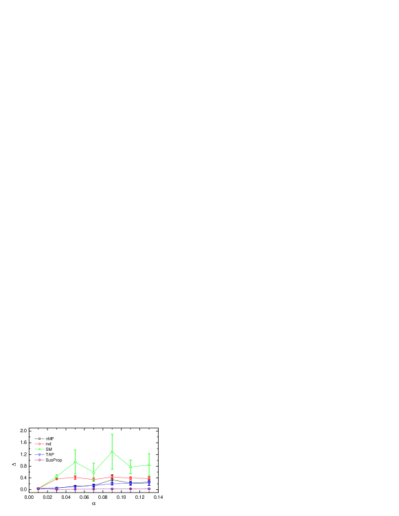
Figure 1: (Color online) Comparison of reconstruction performances of SusProp and other existing mean field schemes in the fully connected Hopfield network. The inference error is plotted against the memory load with $T=0.6,N=100$. Lines are guides to the eye. Each point is an average over five random samples and error bars are also shown.

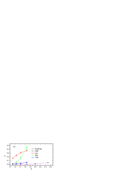
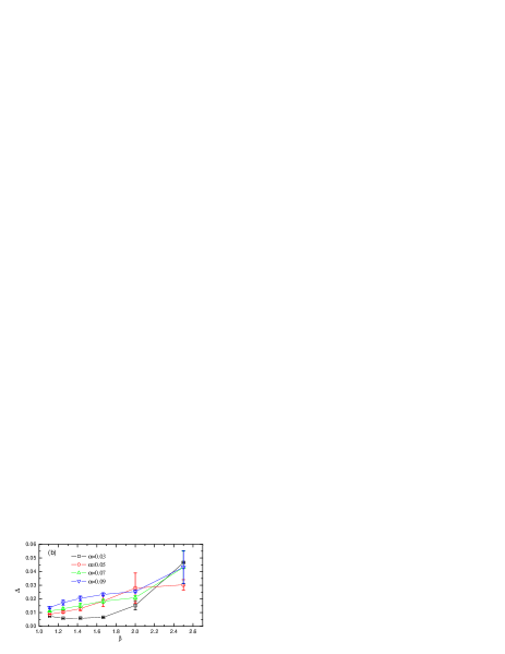
Figure 2: (Color online) The inference error versus temperature for the fully connected network with $N=100$. Lines are guides to the eye. Each point represents an average over five random samples and error bars are also shown. (a) Comparison of reconstruction performances of SusProp and other mean field schemes for $\alpha=0.03$. (b) Inference error versus temperature for SusProp with different memory loads.

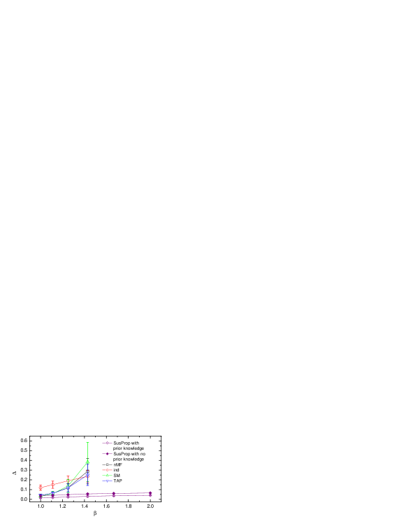
Figure 3: (Color online) Inference performances for the sparse Hopfield network with $\alpha=0.6,l=5,N=100$. Lines are guides to the eye. Each point is an average over five random samples and error bars are also shown. Efficiencies of SusProp and other mean field schemes are compared, so are the reconstruction performances of SusProp with and without prior knowledge on the sparseness of the network.

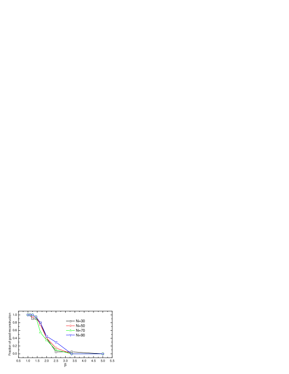
Figure 4: (Color online) Fraction of good reconstruction of fully connected Hopfield networks as a function of inverse temperature $\beta$ for SusProp. Different network sizes are considered with the same memory load $\alpha=0.1$. Twenty random samples are simulated and a good reconstruction is identified when $\Delta\lesssim 0.030$.

IV Reconstruction performances and Discussions

To avoid the expensive computational cost, we assess the reconstruction performance of SusProp only on small size networks. The phase diagram of the Hopfield model has been derived for the fully connected case Amit et al. (1985a, b) and the finite connectivity case Wemmenhove and Coolen (2003). In the finite size system, we distinguish different phases by two order parameters; one is the overlap between the network configuration and the $\mu$th pattern $m^{\mu}=\frac{1}{N}\sum_{i=1}^{N}\xi_{i}^{\mu}m_{i}$ and the other is the mean-squared magnetization $q=\frac{1}{N}\sum_{i=1}^{N}m_{i}^{2}$. To implement SusProp, $\mathcal{T}_{max}$ is set to be $2000$ and we need to adopt an appropriate damping factor to prevent the absolute updated $\tanh J_{ij}$ from being larger than one.

Comparison of reconstruction performances of SusProp and other mean field schemes is shown in Fig. 1. SusProp turns out to be the most efficient, reducing the inference error by a significant amount. Moreover, it seems to be less sensitive to the memory load compared with other mean field methods. Fig. 2 reports the inference error as a function of temperature for various reconstruction algorithms. SusProp operates fairly accurately and extends the reconstructible region well into a much lower temperature down to $0.4$. However, when the system settles in low temperatures ($T<0.6$), SusProp first suffers highly magnetized data and its performance gets worse with non-convergence, which may be remedied by adopting much smaller $\epsilon$ and larger $\mathcal{T}_{max}$ or by introducing a stopping criterion Aurell et al. (2010). When the temperature approaches lower values (e.g., below $0.4$ in Fig. 2 (a)), the collected data will then become frozen, i.e., at least two of its magnetizations equal one in absolute value, as a result, SusProp yields diverging couplings and fails to reconstruct the network. Actually, in the high absolute magnetization case, both $|\widetilde{C_{ij}}|$ and $|m_{i\rightarrow j}|$ (and $|m_{j\rightarrow i}|$) are very close to one on some edges $<ij>$. We then rewrite $\widetilde{C_{ij}}$ as $\widetilde{C_{ij}}={\rm sgn}(\widetilde{C_{ij}})(1-\varepsilon_{ij})$, and similarly $m_{i\rightarrow j}m_{j\rightarrow i}={\rm sgn}(m_{i\rightarrow j}m_{j\rightarrow i})(1-\varepsilon_{ij,ji})$ where ${\rm sgn}(\cdot)$ is a sign function; $\varepsilon_{ij}$ and $\varepsilon_{ij,ji}$ are small positive values compared to one. Then one can readily recast $\tanh J_{ij}$ according to Eq. (5) as

$$\tanh J_{ij}=\frac{{\rm sgn}(\widetilde{C_{ij}})\varepsilon_{ij,ji}-{\rm sgn}(m_{i\rightarrow j}m_{j\rightarrow i})\varepsilon_{ij}}{\varepsilon_{ij,ji}+\varepsilon_{ij}}$$ (7)

for $\widetilde{C_{ij}}m_{i\rightarrow j}m_{j\rightarrow i}>0$ and $|\tanh J_{ij}|=1.0$ for $\widetilde{C_{ij}}m_{i\rightarrow j}m_{j\rightarrow i}<0$. If $\widetilde{C_{ij}}m_{i\rightarrow j}m_{j\rightarrow i}>0$ and neither of $\varepsilon_{ij}$ and $\varepsilon_{ij,ji}$ vanishes, the estimated $J_{ij}$ remains finite and SusProp does work. In other cases (e.g., $|\widetilde{C_{ij}}|=1.0$ and $|m_{i\rightarrow j}m_{j\rightarrow i}|\neq 1.0$), $J_{ij}$ suffers divergence and SusProp is unable to infer the couplings. In this situation, at least two of the supplied magnetizations are equal to one in absolute value, e.g., $|m_{i}|=1.0$ and $|m_{j}|=1.0$, under the update rule Eq. (5), $m_{i\rightarrow j}={\rm sgn}(m_{i})$ and $m_{j\rightarrow i}={\rm sgn}(m_{j})$. These highly polarized messages will then spread out in the network, which yields an infinite value for $J_{ij}$ as explained above. A simple physical interpretation is that, in this case, $\widetilde{C_{ij}}\simeq m_{i}m_{j}$, and this implies that some neurons in the network tend to behave independently of other neurons and thus SusProp couldn’t get all information about correlations of the network, which leads to the failure of reconstruction. In the current Hopfield model, the frozen type data does appear for small enough $\alpha$ and $T$ where the system gets trapped by one of stable or metastable memory states Huang (2010). Increasing $\alpha$ but maintaining low $T$, many spurious minima show up and Monte Carlo sampling becomes very difficult Tokita (1993); Zdeborová (2009), which produces fairly noisy collected data. On the other hand, the current SusProp hasn’t taken into account the complex structure of the phase space, therefore it remains a non-trivial issue for SusProp to deal with this more involved case. The reconstruction error against temperature is also shown with respect to different memory loads for SusProp in Fig. 2 (b). In the high temperature region ($T>0.6$), the smaller the memory load is, the more precisely SusProp reconstructs the Hopfield network. As temperature decreases further, SusProp becomes less precise for all memory loads while still maintaining a relatively small error.

SusProp is applied to reconstruct the fully connected Hopfield network, whereas, it shows a surprisingly good performance. If the network is sparse and locally treelike, SusProp is believed to be fast and able to give a precise estimation. To test its efficiency on reconstructing the sparse network, we compare performances of SusProp with those of other mean field schemes in Fig. 3. It is clearly shown that SusProp performs exceedingly well particularly in the low temperature region (down to $T=0.5$) and exhibits less sample-to-sample fluctuations. If we have a prior knowledge of the sparseness of the network, i.e., we know a priori the connectivity pattern of the network, the inference error could be reduced substantially. In this case, we only infer the strength of interaction between neurons which are really connected. In fact, when the system is presented at the high temperature, one can reconstruct the network using an appropriate cutoff since the estimated couplings between unconnected neurons are very small compared to those between really connected neurons.

In Fig. 4, we report the fraction of good reconstruction versus temperature for different network sizes at fixed memory load $\alpha=0.1$. A good reconstruction is identified when $\Delta\lesssim 0.030$ and SusProp converges within $\mathcal{T}_{max}$. As increasing temperature, a threshold behavior is observed and the transition becomes sharper with growing network size. Given large enough $N$, the probability that SusProp gives good reconstruction tends to be zero when the temperature is below the critical value, and at a high enough temperature, SusProp succeeds in reconstructing the network in all instances. The critical temperature is estimated to be about $0.6$. For a more precise estimation, more samples and larger network size are required. The threshold behavior of SusProp on network reconstruction has also been observed in SK model Aurell et al. (2010).

V Conclusion and outlook

SusProp solves the inverse Ising problem by iteratively updating messages along the directed edges of the network, and is shown in the present work to outperform all other mean-field-type schemes and extend the reconstructible region into lower temperatures. We also study the fraction of good reconstruction as a function of temperature and a threshold behavior is observed. The transition from good reconstruction to poor one becomes sharp as increasing network size and the critical temperature is estimated to be about $0.6$. SusProp is also amazingly efficient for reconstructing sparse Hopfield network and its performance can be further improved by introducing a prior knowledge about the sparseness of the network. The sparse case is more relevant in modeling real biological data than its dense counterpart. We hope our analysis of SusProp on the Hopfield network reconstruction can be extended to the more biologically relevant cases.

At high temperatures, the performance of SusProp is believed to be limited by the quality of the supplied data Marinari and Kerrebroeck (2010). Once the system is presented at the low temperature, the efficiency of SusProp is also determined by the nature of the input data. In the presence of highly magnetized data, the reconstruction performance of SusProp gets deteriorated with a high inference error. Furthermore, the frozen type data makes updated couplings diverge and any value of damping factor can not overcome this hurdle, reminiscent of the fact that the frozen phase in random constraint satisfaction problems is most difficult for any known algorithm Zdeborová and Mézard (2008); Zdeborová (2009).

For large enough $\alpha$ but low enough $T$, the system enters the spin glass phase where Glauber dynamics is easily trapped by one of the spurious minima correlated or uncorrelated with the stored patterns. SusProp fails to extract couplings precisely in this region since it does not take into account the complex structure of the phase space. In fact, at finite temperatures, the support of cavity field distributions becomes real-valued and a sampling procedure is required. On the other hand, other values of Parisi parameter (smaller than the optimal value associated with the ground states) also carry physical information and can be used to describe the metastable states which trap Glauber dynamics Rivoire et al. (2004). However, searching for an optimal Parisi parameter (also known as replica symmetry breaking parameter) is also a time consuming task for the network reconstruction Wemmenhove and Kappen (2006). Rather, provided that Glauber dynamics gets stuck in some metastable state for a very long time, how much information can be extracted from this state about the couplings of the network remains an important issue for future study.

Appendix A Mean field schemes for network reconstruction

A.1 Naive Mean-Field Method

The naive mean field theory gives $m_{i}=\tanh\left(h_{i}+\sum_{k\neq i}J_{ik}m_{k}\right)$ where $h_{i}$ is the external field and $m_{i}=\left<\sigma_{i}\right>$ the magnetization. Using the fluctuation-response relation,

$$C_{ij}=\frac{\partial m_{i}}{\partial h_{j}}=(1-m_{i}^{2})\left[\delta_{ij}+\sum_{k\neq i}J_{ik}C_{kj}\right]$$ (8)

one obtains the nMF prediction of couplings,

$$J_{ij}^{{\rm nMF}}=(\mathbf{P}^{-1})_{ij}-(\mathbf{C}^{-1})_{ij}$$ (9)

where $\mathbf{P}_{ij}=(1-m_{i}^{2})\delta_{ij}$.

A.2 Independent-Pair Approximation

In this approximate scheme, each pair of neurons are independent of other neurons of the system, i.e., their joint probability $P(\sigma_{i},\sigma_{j})\propto\exp\left[h_{i}^{(j)}\sigma_{i}+h_{j}^{(i)}\sigma_{j}+J_{ij}\sigma_{i}\sigma_{j}\right]$ where $h_{i}^{(j)}(h_{j}^{(i)})$ is the local field neuron $i(j)$ feels when neuron $j(i)$ is removed from the system. Then the ind prediction is given by

$$J_{ij}^{{\rm ind}}=\frac{1}{4}\log\left[\frac{(1+C_{ij}^{{}^{\prime}})^{2}-(m_{i}+m_{j})^{2}}{(1-C_{ij}^{{}^{\prime}})^{2}-(m_{i}-m_{j})^{2}}\right]$$ (10)

where $C_{ij}^{{}^{\prime}}=C_{ij}+m_{i}m_{j}$.

A.3 Sessak-Monasson Approximation

The SM prediction of couplings is derived based on a perturbative expansion in the correlations Sessak and Monasson (2009) and it can be formulated as

$$J_{ij}^{{\rm SM}}=J_{ij}^{{\rm nMF}}+J_{ij}^{{\rm ind}}-\frac{C_{ij}}{(1-m_{i}^{2})(1-m_{j}^{2})-C_{ij}^{2}}$$ (11)

A.4 Inversion of TAP Equations

The usual TAP equation reads $h_{i}=\tanh^{-1}m_{i}-\sum_{j\neq i}J_{ij}m_{j}+m_{i}\sum_{j\neq i}J_{ij}^{2}(1-m_{j}^{2})$ Mézard et al. (1987). Differentiating the field $h_{i}$ with respect to the magnetization $m_{j}$, one readily obtains the TAP prediction equation,

$$(\mathbf{C}^{-1})_{ij}=\frac{\partial h_{i}}{\partial m_{j}}=-J_{ij}^{{\rm TAP}}-2(J_{ij}^{{\rm TAP}})^{2}m_{i}m_{j}$$ (12)

Appendix B Simulation details

The rule for Glauber dynamics can be generally expressed as $P(\sigma_{i}\rightarrow-\sigma_{i})=\frac{1}{1+\exp(\beta\Delta\mathcal{H}_{i})}$ where $\Delta\mathcal{H}_{i}$ is the energy change due to such a flip. For the current Hopfield model, the dynamics rule is recast into

$$P(\sigma_{i}\rightarrow-\sigma_{i})=\frac{1}{2}\left[1-\sigma_{i}\tanh\beta h_{i}\right]$$ (13)

where $\beta$ is the inverse temperature and $h_{i}=\sum_{j\neq i}J_{ij}\sigma_{j}$ is the local field acting on $\sigma_{i}$.

In our numerical simulations, we update the state of each neuron according to Eq. 13 in a randomly asynchronous manner. We define a Glauber dynamics step as $N$ proposed flips. Introducing simulated annealing strategy, we set the initial temperature to be $1.0$ and the cooling rate $0.005$. At each intermediate temperature, we run $10^{4}$ Glauber dynamics steps. When the temperature is decreased to the desired one, we run another $2\times 10^{6}$ steps to calculate magnetizations and correlations. We sample the state of the network every $200$ steps. For high temperatures ($\geq 1.0$), we run totally $4\times 10^{6}$ steps, among which the first $2\times 10^{6}$ steps are run for the system to reach the equilibrium state and the other $2\times 10^{6}$ steps for calculating magnetizations and correlations.

Appendix C Derivation of SusProp update rules

To derive Eq. 5, we first derive the susceptibility propagation equations for general $K$-body interaction problem ($K=2$ for the Hopfield model). Using the factor graph representation Kschischang et al. (2001), we denote $a$ as the function node representing the constraint imposed on a subset of spins $\boldsymbol{\sigma}_{\partial a}$ ($\partial a$ denotes neighbors of the function node $a$), and $i$ as variable node representing the spin on the factor graph. The belief propagation is then formulated as Huang and Zhou (2009)

$$\begin{split}m_{i\rightarrow a}&\equiv\tanh h_{i\rightarrow a}=\tanh\left(\sum_{b\in\partial i\backslash a}u_{b\rightarrow i}\right)=\tanh\left[\tanh^{-1}(m_{i})-u_{a\rightarrow i}\right]\\ &=\frac{m_{i}-\tanh J_{a}\prod_{j\in\partial a\backslash i}m_{j\rightarrow a}}{1-m_{i}\tanh J_{a}\prod_{j\in\partial a\backslash i}m_{j\rightarrow a}}\end{split}$$ (14a)

$$\tanh u_{b\rightarrow i} =\tanh J_{b}\prod_{j\in\partial b\backslash i}m_{j\rightarrow b}$$ (14b)

where $h_{i\rightarrow a}$ is the cavity field (correspondingly $m_{i\rightarrow a}$ is the cavity magnetization) acting on spin $\sigma_{i}$ in the absence of $a$; $u_{b\rightarrow i}$ the cavity bias when $i$ is involved in $b$ only, and $h_{i\rightarrow a},u_{b\rightarrow i}$ as well as $J_{b}$ have been rescaled by $\beta$.

We define cavity susceptibility $g_{i\rightarrow a,k}\equiv\frac{\partial h_{i\rightarrow a}}{\partial h_{k}}$. From the belief propagation equations, one readily gets the update rule for $g_{i\rightarrow a,k}$:

$$\begin{split}g_{i\rightarrow a,k}&=\delta_{ik}+\sum_{b\in\partial i\backslash a}\frac{\partial u_{b\rightarrow i}}{\partial h_{k}}\\ &=\delta_{ik}+\sum_{b\in\partial i\backslash a}\frac{\tanh J_{b}}{1-\left(\tanh J_{b}\prod_{j\in\partial b\backslash i}m_{j\rightarrow b}\right)^{2}}\sum_{j\in\partial b\backslash i}\left[\prod_{n\in\partial b\backslash i,j}m_{n\rightarrow b}\right]g_{j\rightarrow b,k}(1-m_{j\rightarrow b}^{2})\end{split}$$ (15)

Using the identity Higuchi and Mézard (2010):

$$\frac{\partial u_{a\rightarrow i}\left(\{h_{j\rightarrow a}\}_{j\in\partial a\backslash i}\right)}{\partial{h_{n\rightarrow a}}}=\frac{\left<\sigma_{n}\sigma_{i}\right>-\left<\sigma_{n}\right>\left<\sigma_{i}\right>}{1-\left<\sigma_{i}\right>^{2}}$$ (16)

where $i,n\in\partial a$ and $\left<\cdots\right>$ denotes the average under the joint probability distribution ${\rm Prob}(\boldsymbol{\sigma}_{\partial a})$ which can be computed from the belief propagation equations, one can re-express the correlations $C_{ij}$ through the fluctuation-response relation:

$$\begin{split}C_{ij}&=\frac{\partial m_{i}}{\partial h_{j}}=(1-m_{i}^{2})\left[\delta_{ij}+\sum_{b\in\partial i}\frac{\partial u_{b\rightarrow i}}{\partial h_{j}}\right]\\ &=(1-m_{i}^{2})\left[g_{i\rightarrow a,j}+\sum_{n\in\partial a\backslash i}\frac{\partial u_{a\rightarrow i}}{\partial h_{n\rightarrow a}}\frac{\partial h_{n\rightarrow a}}{\partial h_{j}}\right]\\ &=(1-m_{i}^{2})\left[g_{i\rightarrow a,j}+\sum_{n\in\partial a\backslash i}\frac{\partial u_{a\rightarrow i}}{\partial h_{n\rightarrow a}}g_{n\rightarrow a,j}\right]\end{split}$$ (17)

For the simple case, the Hopfield network, $J_{a}=J_{ij}$, and the constraint $a$ involves only two neurons, say $i$ and $j$. To obtain the update rule for $J_{ij}$, we compute $\widetilde{C_{ij}}\equiv\left<\sigma_{i}\sigma_{j}\right>$ directly by assuming ${\rm Prob}(\sigma_{i},\sigma_{j})\propto\exp\left(J_{ij}\sigma_{i}\sigma_{j}+h_{i\rightarrow j}\sigma_{i}+h_{j\rightarrow i}\sigma_{j}\right)$, finally we get

$$\tanh J_{ij}=\frac{\widetilde{C_{ij}}-m_{i\rightarrow j}m_{j\rightarrow i}}{1-\widetilde{C_{ij}}m_{i\rightarrow j}m_{j\rightarrow i}}$$ (18)

where $\widetilde{C_{ij}}$ can be evaluated from Eqs. 16 and 17, i.e.,

$$\widetilde{C_{ij}}=\frac{C_{ij}-(1-m_{i}^{2})g_{i\rightarrow j,j}}{g_{j\rightarrow i,j}}+m_{i}m_{j}$$ (19)

From Eqs. 14 and  15, the update rules for $m_{i\rightarrow j}$ and $g_{i\rightarrow j,k}$ are finally obtained as follows,

$$m_{i\rightarrow j} =\frac{m_{i}-m_{j\rightarrow i}\tanh J_{ij}}{1-m_{i}m_{j\rightarrow i}\tanh J_{ij}}$$ (20a)

$$g_{i\rightarrow j,k} =\delta_{ik}+\sum_{n\in\partial i\backslash j}\frac{1-m_{n\rightarrow i}^{2}}{1-(m_{n\rightarrow i}\tanh J_{ni})^{2}}\tanh J_{ni}g_{n\rightarrow i,k}$$ (20b)

Introducing additionally a damping factor $\epsilon$, Eqs. 18, 19 and 20 are the very SusProp we have presented in Sec. III.

References

- Mézard et al. (2002) M. Mézard, G. Parisi, and R. Zecchina, Science 297, 812 (2002).
- Braunstein and Zecchina (2006) A. Braunstein and R. Zecchina, Phys. Rev. Lett 96, 030201 (2006).
- Richardson and Urbanke (2001) T. J. Richardson and R. L. Urbanke, IEEE Trans. Inf. Theory 47, 599 (2001).
- Huang and Zhou (2009) H. Huang and H. Zhou, Phys. Rev. E 80, 056113 (2009).
- Mézard and Mora (2009) M. Mézard and T. Mora, J. Physiology Paris 103, 107 (2009).
- Aurell et al. (2010) E. Aurell, C. Ollion, and Y. Roudi, arXiv:1005.3694 (2010), [Eur. Phys. J. B (in press)].
- Marinari and Kerrebroeck (2010) E. Marinari and V. V. Kerrebroeck, J. Stat. Mech.: Theory Exp P02008 (2010).
- Shlens et al. (2006) J. Shlens, G. D. Field, J. L. Gauthier, M. I. Grivich, D. Petrusca, A. Sher, A. M. Litke, and E. J. Chichilnisky, J. Neurosci 26, 8254 (2006).
- Pillow et al. (2008) J. W. Pillow, J. Shlens, L. Paninski, A. Sher, A. M. Litke, E. J. Chichilnisky, and E. P. Simoncelli, Nature 454, 995 (2008).
- Shlens et al. (2009) J. Shlens, G. D. Field, J. L. Gauthier, M. Greschner, A. Sher, A. M. Litke, and E. J. Chichilnisky, J. Neurosci 29, 5022 (2009).
- Tang et al. (2008) A. Tang, D. Jackson, J. Hobbs, W. Chen, J. L. Smith, H. Patel, A. Prieto, D. Petrusca, M. I. Grivich, A. Sher, et al., J. Neurosci 28, 505 (2008).
- Ohiorhenuan et al. (2010) I. E. Ohiorhenuan, F. Mechler, K. P. Purpura, A. M. Schmid, Q. Hu, and J. D. Victor, Nature 466, 617 (2010).
- Lezon et al. (2006) T. R. Lezon, J. R. Banavar, M. Cieplak, A. Maritan, and N. V. Fedoroff, Proc. Natl. Acad. Sci. USA 103, 19033 (2006).
- Seno et al. (2008) F. Seno, A. Trovato, J. R. Banavar, and A. Maritan, Phys. Rev. Lett 100, 078102 (2008).
- Mora et al. (2010) T. Mora, A. M. Walczak, W. Bialek, and J. C. G. Callan, Proc. Natl. Acad. Sci. USA 107, 5405 (2010).
- Schneidman et al. (2006) E. Schneidman, M. J. Berry, R. Segev, and W. Bialek, Nature 440, 1007 (2006).
- Tkacik et al. (2009) G. Tkacik, E. Schneidman, M. J. Berry, and W. Bialek (2009), e-print arXiv:0912.5409.
- Cocco et al. (2009) S. Cocco, S. Leibler, and R. Monasson, Proc. Natl. Acad. Sci. USA 106, 14058 (2009).
- Weigt et al. (2009) M. Weigt, R. A. White, H. Szurmant, J. A. Hoch, and T. Hwa, Proc. Natl. Acad. Sci. USA 106, 67 (2009).
- Roudi et al. (2009a) Y. Roudi, E. Aurell, and J. Hertz, Front. Comput. Neurosci 3, 1 (2009a).
- Ackley et al. (1985) D. H. Ackley, G. E. Hinton, and T. J. Sejnowski, Cognitive Science 9, 147 (1985).
- Hinton and Sejnowski (1986) G. E. Hinton and T. J. Sejnowski, in Parallel Distributed Processing: Explorations in the Microstructure of Cognition, edited by D. E. Rumelhart, J. L. McClelland, and the PDP Research Group (MIT Press, Cambridge, 1986), vol. 1, pp. 282–317.
- Hertz et al. (1991) J. Hertz, A. Krogh, and R. G. Palmer, Introduction to the Theory of Neural Computation (Addison-Wesley, Redwood City, 1991).
- Kschischang et al. (2001) F. R. Kschischang, B. J. Frey, and H.-A. Loeliger, IEEE Trans. Inf. Theory 47, 498 (2001).
- Higuchi and Mézard (2010) S. Higuchi and M. Mézard, J. Phys.: Conf. Ser 233, 012003 (2010).
- Huang (2010) H. Huang, Phys. Rev. E 81, 036104 (2010).
- Roudi et al. (2009b) Y. Roudi, J. Tyrcha, and J. Hertz, Phys. Rev. E 79, 051915 (2009b).
- Zhang et al. (2010) P. Zhang, A. Ramezanpour, and R. Zecchina (2010), to be submitted.
- Hopfield (1982) J. J. Hopfield, Proc. Natl. Acad. Sci. USA 79, 2554 (1982).
- Amit (1989) D. J. Amit, Modeling Brain Function: The World of Attractor Neural Networks (Cambridge University Press, Cambridge, 1989).
- Amit et al. (1985a) D. J. Amit, H. Gutfreund, and H. Sompolinsky, Phys. Rev. Lett 55, 1530 (1985a).
- Amit et al. (1985b) D. J. Amit, H. Gutfreund, and H. Sompolinsky, Phys. Rev. A 32, 1007 (1985b).
- Tokita (1993) K. Tokita, J. Phys. A 26, 6915 (1993).
- Wemmenhove and Coolen (2003) B. Wemmenhove and A. C. C. Coolen, J. Phys. A 36, 9617 (2003).
- Castillo and Skantzos (2004) I. P. Castillo and N. S. Skantzos, J. Phys. A 37, 9087 (2004).
- Watkin and Sherrington (1991) T. L. H. Watkin and D. Sherrington, Europhys. Lett 14, 791 (1991).
- Canning and Naef (1992) A. Canning and J. P. Naef, J. Physique I 2, 1791 (1992).
- Zdeborová (2009) L. Zdeborová, Acta Physica Slovaca 59, 169 (2009).
- Zdeborová and Mézard (2008) L. Zdeborová and M. Mézard, Phys. Rev. Lett 101, 078702 (2008).
- Rivoire et al. (2004) O. Rivoire, G. Biroli, O. C. Martin, and M. Mézard, Eur. Phys. J. B 37, 55 (2004).
- Wemmenhove and Kappen (2006) B. Wemmenhove and H. J. Kappen, J. Phys. A 39, 1265 (2006).
- Sessak and Monasson (2009) V. Sessak and R. Monasson, J. Phys. A 42, 055001 (2009).
- Mézard et al. (1987) M. Mézard, G. Parisi, and M. A. Virasoro, Spin Glass Theory and Beyond (World Scientific, Singapore, 1987).