The Crab Nebula as a standard candle in
very high-energy astrophysics

Abstract

The continuum high-energy gamma-ray emission between $1$ GeV and $10^{5}$ GeV from the Crab Nebula has been measured for the first time in overlapping energy bands by the Fermi large-area telescope (Fermi/LAT) below $\approx 100$ GeV and by ground-based imaging air Cherenkov telescopes (IACTs) above $\approx 60$ GeV. To follow up on the phenomenological approach suggested by Hillas et al. (1998), the broad band spectral and spatial measurement (from radio to low-energy gamma-rays $<1$ GeV) is used to extract the shape of the electron spectrum. While this model per construction provides an excellent description of the data at energies $<1$ GeV, the predicted inverse Compton component matches the combined Fermi/LAT and IACT measurements remarkably well after including all relevant seed photon fields and fitting the average magnetic field to $B=\left(124\,{}\pm 6\,\mathrm{(stat.)}\,{}^{+15}_{-6}\,\mathrm{(sys.)}\right)\,\mu\mathrm{G}$. The close match of the resulting broad band inverse Compton component with the combined Fermi/LAT and IACTs data is used to derive instrument specific energy-calibration factors. These factors can be used to combine data from Fermi/LAT and IACTs without suffering from systematic uncertainties on the common energy scale. As a first application of the cross calibration, we derive an upper limit to the diffuse gamma-ray emission between 250 GeV and 1 TeV based upon the combined measurements of Fermi/LAT and the H.E.S.S. ground-based Cherenkov telescopes. Finally, the predictions of the magneto-hydrodynamic flow model of Kennel & Coroniti (1984) are compared to the measured SED.

I Introduction

The Crab Nebula has been and remains an intensely studied object in astrophysics (for a recent review see e.g. Hester 2008). It is part of the remnant of a core-collapse supernova that occurred in 1054 AD at a distance of $d\approx 2\,\mathrm{kpc}$ (Trimble 1968). Observations of the nebula have been carried out at every accessible wavelength resulting in a remarkably well-determined spectral energy distribution (SED). Therefore, the Crab Nebula is an ideal object for detailed studies of the conversion of Poynting flux to particle energy flux (see e.g. Coroniti 1990; Kirk & Skjæraasen 2003; Arons 2008) and finally of the acceleration processes taking place at the termination shock (see e.g. Emmering & Chevalier 1987; Spitkovsky & Arons 2004). The commonly considered model for the Crab Nebula (see e.g. Rees & Gunn 1974, henceforth RG74) assumes an ultra-relativistic outflow from the pulsar that terminates in a standing shock at a distance $r_{s}$ which is roughly 10% of the total nebula’s size. In the downstream medium, the particles are pitch-angle isotropized, forming a broad power law in energy. The magneto-hydrodynamic (MHD) analysis of the downstream flow by Kennel & Coroniti (1984), henceforth KC84, provides an elegant solution to the particle distribution and the magnetic field downstream of the shock under the assumption of a particular ad hoc injection spectrum. In the framework of this model, the radio emission is explained by a separate electron population, which has been linked to the high spin-down phase of the pulsar (relic electrons, Atoyan 1999) or by acceleration in MHD turbulences (Nodes et al. 2004).

Several different models have been proposed to explain the observed high-energy gamma-rays as inverse Compton emission from the same electron population responsible for the synchrotron X-ray emission (see, e.g., de Jager & Harding 1992; Atoyan & Aharonian 1996; Hillas et al. 1998; Bednarek & Bartosik 2003; Aharonian et al. 2004; Zhang et al. 2008; Volpi et al. 2008. We point out that Volpi et al. use a time-dependent axisymmetric numerical simulation of the nebula’s evolution). The large uncertainties in the observational data in the past have only weakly constrained the models at high energies, i.e., between 1 GeV and 100 GeV. The largely improved statistics of the measurements carried out with the recently commissioned Fermi/LAT (Atwood et al. 2009) have provided us with more accurate data in this crucial energy window. Nevertheless, the combined observations carried out with different instruments in overlapping energy bands (Fermi/LAT and IACTs) are currently limited by the systematic uncertainties of the relative and absolute energy calibration.

Because of this, a two-pronged approach is followed here. On the one hand, we perform accurate modeling of the available measurements of the broad band SED of the Crab Nebula. On the other, the model is used to derive corrections of the measured energy scale for the individual instruments to a common energy scale. This cross calibration reduces the systematic uncertainties and proves useful for any study which relies on the combination of spectral measurements of the Fermi/LAT and IACTs.

Given that we are mainly interested in the spectral modeling of the high-energy emission, which is currently not spatially resolvable, we primarily apply a simple and robust approach based upon the work of Hillas et al. (1998), which we refer to as the constant B-field model. Nevertheless, we also investigate the MHD flow model suggested by KC84 and its application to the inverse Compton component (Atoyan & Aharonian 1996, henceforth AA96).

The article is organized as follows. In Section II the available data and modeling of the SED are presented and discussed. Both, the simplified constant B-field model and the MHD flow model of KC84 are fitted to the measured synchrotron part of the SED by means of a $\chi^{2}$-minimization. The results of the two models are compared. In Section III, we discuss the properties of the underlying electron spectrum of the simplified model as derived from the observations. The results of a first instrumental cross calibration are presented in Section IV, together with an application to extract limits on the diffuse $\gamma$-ray background at TeV energies.

II Spectral energy distribution of the Crab Nebula

The compilation of observational data used here is summarized by Aharonian et al. (2004) and references therein. The radio data (Macías-Pérez et al. 2010) have been corrected for a secular decline of $-0.18~{}\%/$yr to a common date (01/01/2000). Additionally, new data are added and listed in Table 1, while the entire compilation of data is displayed in Fig. 1(a) and 1(b). The far infrared (FIR) observations from Spitzer, ISO, and Scuba deviate from a simple power-law extrapolation of the radio spectrum. The flux of the optical line emission is taken from Davidson & Fesen (1985), Davidson (1987) and Hester et al. (1990). The optical line emission of the filaments in the nebula is estimated in the following way. The high-resolution spectral observations of individual filaments have been corrected for extinction (Hester et al. 1990) and scaled to match the global emission from the filaments (see the discussion in Davidson & Fesen 1985).

New X-ray observations by the XMM-Newton and INTEGRAL observatories have been chosen to replace older measurements. Both, the XMM-Newton and INTEGRAL (with the instruments SPI and IBIS/ISGRI) observatories are calibrated on the basis of detailed simulations and laboratory measurements (Gondoin et al. 1998a, b; Attié et al. 2003). This approach differs from commonly used methods in which corrections of the instrument’s response function are applied to reproduce a specific spectral shape and flux of the Crab Nebula. As a result, corrected measurements are model-dependent and therefore we chose not to include them here. The cameras of XMM-Newton spatially resolve the Crab Nebula, whereas the measurements of SPI and IBIS/ISGRI may include contributions from the pulsar, possibly leading to higher fluxes in comparison to the XMM-Newton observations. We stress that the difference in flux normalization between XMM-Newton and SPI are beyond the systematic errors quoted. To combine the two measurements, we chose to scale the flux of the SPI data by a factor of $0.78$ to match the extrapolation of the measurement of XMM-Newton.

Table 1: Observations used for the SED. All other data shown in Fig. 1(a),1(b) are taken from Aharonian et al. (2004) and references therein. (1) Green et al. (2004); (2) Temim et al. (2006); (3) Kirsch et al. (2005); (4) Jourdain & Roques (2009); (5) Jourdain et al. (2008); (6) Abdo et al. (2010); (7) Aharonian et al. (2006); (8) Albert et al. (2008)

Energy Band	Instrument	Reference
Submillimeter	ISO & SCUBA	(1)
to far infrared	SPITZER	(2)
X-ray to	XMM-Newton	(3)
$\gamma$-ray	SPI	(4)
	IBIS$/$ISGRI	(5)
	Fermi / LAT	(6)
VHE	H.E.S.S.	(7)
	MAGIC	(8)

II.1 Constant B-field model

The nebula is assumed to be filled with relativistic electrons with an averaged total differential number $\mathrm{d}N_{\mathrm{el}}/\mathrm{d}\gamma$. To explain the change in the continuum between the radio and infrared (see above), we distinguish between radio and wind electrons. The two spectra are assumed to follow power laws with appropriate cut-offs. For the radio-emitting electrons, a power law between $\gamma^{r}_{\mathrm{min}}=22$ (a value only constrained towards higher values of $\gamma$ and kept constant in the fit), and $\gamma^{r}_{\mathrm{max}}$

$$\frac{\mathrm{d}N_{\mathrm{el}}^{r}}{\mathrm{d}\gamma} = \left\{\begin{array}[]{ll}N_{0}^{r}\gamma^{-S_{r}}&\mathrm{for}\quad\gamma^{r}_{\mathrm{min}}\leq\gamma\leq\gamma^{r}_{\mathrm{max}},\\ \\ 0&\mathrm{otherwise},\end{array}\right.$$ (4)

is sufficient, while for the wind electrons a broken power law with a superexponential cut-off at the lower end is required:

$$\frac{\mathrm{d}N_{\mathrm{el}}^{w}}{\mathrm{d}\gamma} = N_{0}^{w}\left\{\begin{array}[]{ll}\left(\frac{\gamma}{\gamma_{\mathrm{break}}^{w}}\right)^{-S_{w}},&\mathrm{for}\quad\gamma<\gamma_{\mathrm{break}}^{w},\\ \\ \left(\frac{\gamma}{\gamma_{\mathrm{break}}^{w}}\right)^{-(S_{w}+\Delta S)},&\mathrm{for}\quad\gamma^{w}_{\mathrm{break}}\leq\gamma\leq\gamma_{\mathrm{max}}^{w},\\ \\ 0,&\mathrm{for}\quad\gamma>\gamma^{w}_{\mathrm{max}},\\ \end{array}\right\}$$ (10)

$$\quad\times\exp\left(-\left[\frac{\gamma_{\mathrm{min}}^{w}}{\gamma}\right]^{\beta}\right).$$

As assumed by Hillas et al. (1998), the electron-number volume density $n_{\mathrm{el}}^{w}(\gamma,r)$ in the nebula is taken to drop off radially following a Gaussian function such that

$$n_{\mathrm{el}}^{w}(\gamma,r) = \frac{n^{w}_{0}}{N_{0}^{w}}\exp\left[-\frac{r^{2}}{2\rho^{2}(\gamma)}\right]\frac{\mathrm{d}N_{\mathrm{el}}^{w}}{\mathrm{d}\gamma}.$$ (11)

The width of the Gaussian $\rho(\gamma)$ decreases with increasing Lorentz factor $\gamma$ to account for the observed shrinking of the nebula (see Appendix A for further details). The volume of the nebula is assumed to be filled with an entangled magnetic field of constant field strength. Within the nebula, various seed photon fields are upscattered by the electrons via the inverse Compton process. The effective density of seed photons $n_{\mathrm{seed}}$ is calculated by convolving the electron density with the photon density and summing the contributions from several different components: (1) synchrotron radiation, (2) emission from thermal dust, (3) the cosmic microwave background radiation (CMB), and (4) optical line emission from the nebula’s filaments. Similar to the electron population, the spatial photon densities are approximated by (energy-dependent) Gaussian distributions, whereas the photon density of the CMB is assumed to be constant throughout the nebula. The relevant relations for the seed photon fields are summarized in Appendix A (for further details see also Hillas et al. 1998). The resulting synchrotron and inverse Compton emission (at frequency $\nu$) is found by

$$L_{\nu} = \int\limits_{1}^{\infty}\mathrm{d}\gamma\frac{\mathrm{d}N_{\mathrm{el}}}{\mathrm{d}\gamma}\left(\mathcal{L}_{\nu}^{\mathrm{Sy}}+\mathcal{L}_{\nu}^{\mathrm{IC}}\right).$$ (12)

The specific single particle emission functions $\mathcal{L}_{\nu}$ for synchrotron (Sy) and inverse Compton (IC) processes are given in Appendix B.

For a given value of the magnetic field, the shapes of the two electron spectra are varied until the resulting synchrotron spectrum reproduces the observational data. The best-fit values for the ten free parameters describing the electron spectrum at a fixed magnetic field strength are determined by means of a least-squares algorithm (Levenberg-Marquardt), which provides the closest match of the expected synchrotron spectrum (between $1$ and $10^{14}$ GHz) with the observational data (see Table 2 for the results of the fit and the discussion in Section III). The resulting $\chi^{2}/\mathrm{d.o.f}=214.5/217$ is below unity after a relative systematic uncertainty of $7$ % was added in quadrature to the statistical error quoted for the data in the literature. The minimization procedure is not sensitive to the particular choice of starting values and it converges reliably. The resulting covariance matrix allows for an analysis of the correlations between various parameters. As expected, the normalizations are anti-correlated to the power law indices. Additionally, there are modest anti-correlations between the position of the break in the spectrum of the wind-electrons with the power-law indices. The matrix of correlation coefficients is listed in Appendix C.

The predicted inverse Compton component above 700 MeV is then used to calculate $\chi^{2}(B)$ for a range of $B$-field values using only the Fermi data. The best-fit value of $B$ and its statistical uncertainties are estimated by adjusting a parabola to $\chi^{2}(B)$ and calculating its second derivative. After taking the systematic energy uncertainty on the global energy scale of the Fermi/LAT data into account, $\Delta E/E={}^{+5\%}_{-10\%}$ (see e.g. Abdo et al. 2009), the average $B$-field is found to be

$$B=\left(124\,{}\pm 6\,\mathrm{(stat.)}\,{}^{+15}_{-6}\,\mathrm{(sys.)}\right)\,\mu\mathrm{G}.$$ (13)

The reduced $\chi^{2}/\mathrm{d.o.f.}=6.37/13\approx 0.49$ for the fit of the inverse Compton component to the Fermi data indicates that the statistical errors on the Fermi differential flux may be slightly overestimated.

The resulting broad band SED is displayed in Fig. 1(a) ( solid and dashed blue curves) including synchrotron and IC emission and thermal emission from the dust in the nebula and optical line emission from the filaments (dashed magenta line). The inverse Compton component including the various contributions of different seed photon fields is shown in detail in Fig. 2. For convenience, an analytical parametrization of the derived energy flux above $1$ GeV is presented in Appendix D. This parametrization is especially useful to derive cross calibration factors as introduced in Section IV for other or future instruments that measure the same energy range.

For the thermal dust emission a graybody spectrum is used. By fitting the combined spectrum (thermal and nonthermal emission) to the data a temperature of $T=93\,\mathrm{K}$ is derived. The graybody peaks at $(\nu f_{\nu})_{\mathrm{max}}\approx 6.45\times 10^{~{}-9}\,\mathrm{ergs}\,\mathrm{s}^{-1}\,\mathrm{cm}^{-2}$. With the relation (Gehrz et al. 1998)

$$M_{\mathrm{dust}}=\frac{1.36(\nu f_{\nu})_{\mathrm{max}}~{}a\rho~{}4\pi d^{2}}{3\sigma_{\mathrm{SB}}T^{4}},$$ (14)

the dust mass $M_{\mathrm{dust}}$ can be estimated. Here $\sigma_{\mathrm{SB}}$ denotes the Stefan-Boltzmann constant. We adopt the same assumptions as Temim et al. (2006); i.e., we assume a dust grain size of $a=10\,\mu\mathrm{m}$ and graphite grains with a density of $\rho=2.25\,\mathrm{g}\,\mathrm{cm}^{~{}-3}$. This leads to a dust mass of $M_{\mathrm{dust}}=4\times 10^{-4}M_{\odot}$, about 40% of the value obtained by Temim et al. (2006).

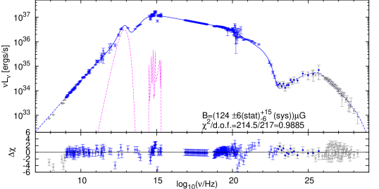
(a) The SED of the Crab nebula calculated in the framework of the constant B-field model. The open blue data points have been included in the fit for the synchrotron part and the filled blue points used to determine the best-fitting magnetic field.

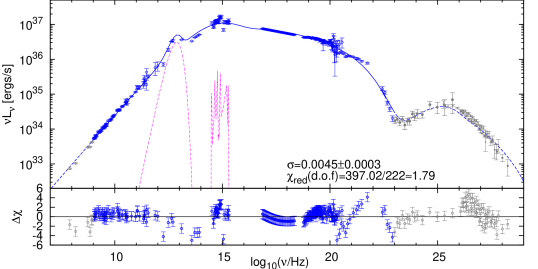
(b) The SED of the Crab nebula (data identical to Fig. 1(a)) with a best-fit model using an MHD flow description of the pulsar wind nebula.

Figure 1: The SEDs for the constant B-field and MHD flow model. The data compilation is based upon Aharonian et al. (2004) with updates listed in Table 1 and modifications (e.g. scaling of the SPI flux) described in the text. See Section II for further details. The synchrotron emission fitted to the data is shown by the blue solid line while the remaining components (low energy part and inverse Compton emission) naturally result from the model. Therefore, blue data points have been included in the fit whereas the gray points have been excluded. In addition to the nonthermal continuum emission, the contribution of dust and line emission from the filaments is indicated with a magenta dashed line. The lower panels show the residuals of the fit. .

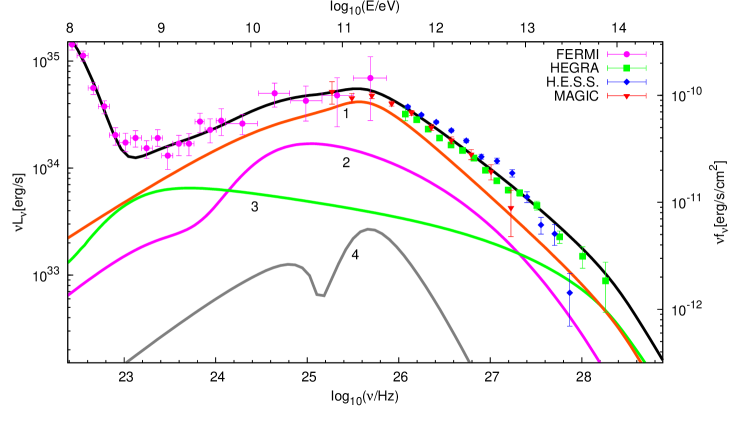
Figure 2: The Fermi/LAT and IACT data points are shown along with the total IC flux of the constant B-field (black line) and individual components from the different seed photon fields (constant B-field model): (1) synchrotron, (2) thermal dust, (3) CMB, and (4) line emission from filaments.

II.2 MHD flow model

While the treatment presented above provides an accurate match of the measured broad band SED, a more physical description of the evolution of the injected particles and magnetic field in a spherical volume has been suggested by KC84. In addition to the synchrotron component already studied by KC84, AA96 extended this approach by investigating the high-energy (inverse Compton) component of the SED. The MHD solution requires the shock distance $r_{s}$, the magnetization parameter $\sigma$, i.e. the ratio of the Poynting flux to the particle energy flux at the position of the shock, and the shape of the injected electron spectrum (particle number per unit volume $n(\gamma)$ in the interval $\gamma$ to $\gamma+d\gamma$) as main input parameters.

Previously, RG74 assumed a shock distance of $r_{\mathrm{s}}=0.10~{}\,\mathrm{pc}$, which in the meantime has become the canonical value, whereas recent high spatial resolution Chandra observations (Weisskopf et al. 2000) indicate that the shock (if identified with the bright inner ring in the X-ray image at $14"$ distance to the pulsar) resides at a distance of $r_{\mathrm{s}}=(0.14\pm 0.01)\,\mathrm{pc}$.

Based upon the initial analysis of KC84, the magnetization paramater was considered to be less than 1% with typical values ranging from $\sigma=0.001$ to $\sigma=0.005$. With such low values of $\sigma$, both the observed break in the spectrum between optical and radio wavelengths and the general morphology of the nebula are reproduced for the most part. However, the asymmetry in the brightness of the far and near sides of the torus observed in X-rays and the measured flow speed (Mori et al. 2004) imply a higher value of $\sigma$ between $0.01$ and $0.13$, more likely close to $\sigma=0.05$ (Shibata et al. 2003; Mori et al. 2004).

Following the approach suggested by AA96, the broad band SED is calculated (see Eq. 12) including the same external seed photon fields as described above and two populations of electrons. The radio-emitting relic electrons are distributed homogeneously in the nebula with

$$n_{\mathrm{radio}}(\gamma)=n_{0}\gamma^{-S_{r}}~{}\exp\left(-\frac{\gamma}{\gamma_{\mathrm{max}}^{r}}\right),$$ (15)

whereas a population of wind electrons is injected at the shock:

$$n_{\mathrm{wind}}(\gamma) = q_{0}(\gamma+\gamma^{w}_{\mathrm{min}})^{-S_{w}}\exp\left(-\frac{\gamma}{\gamma_{\mathrm{max}}^{w}}\right).$$ (16)

The radiative and adiabatic cooling of the wind electrons is treated in the same way as suggested by AA96. The best-fitting value for the seven parameters describing the electron spectra are found in a similar way to what is described above. For a fixed value of $\sigma$, the parameters describing the electron distribution ($n_{0}$, $S_{r}$, $\gamma_{\mathrm{max}}^{r}$, $q_{0}$, $\gamma^{w}_{\mathrm{min}}$, $S_{w}$, $\gamma_{\mathrm{max}}^{w}$) are varied, until the predicted synchrotron emission is matched best to the same data as used for the constant B-field model. The procedure is repeated for a range of values of $\sigma$ until an absolute minimum is found at $\sigma=0.0045\pm 0.0003$ and $\chi^{2}/\mathrm{d.o.f.}=397.02/222\approx 1.79$ with a probability of obtaining a higher value of $\chi^{2}$ per chance $P(>\chi^{2})=4.8\times 10^{-12}$ (see Table 3 for the best-fit values and Appendix C for the correlation coefficients). The high $\chi^{2}$ value indicates that the simple MHD-flow model fails to describe the synchrotron part of the SED in detail, while the overall shape is certainly correct. It is noteworthy that the high value of $\gamma^{r}_{\mathrm{max}}$ implies that most of the optical emission is produced by the same population of electrons as are responsible for the radio emission. In this case, the spatial extension predicted at optical frequencies would be similar to the extension of the radio nebula which clearly contradicts observations. When looking at the inverse Compton component calculated in this model, the agreement between the Fermi part of the spectrum and the model is fairly good, even though the shape of the synchrotron cut-off is harder than the measured spectrum. At energies beyond the position of the peak in the inverse Compton part of the SED, the model spectra are considerably harder than the actual measurements. The discrepancy is directly related to the mismatch that is evident in the X-ray part of the synchrotron spectrum.

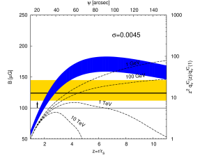
Figure 3: The black horizontal line and the yellow shaded region mark the volume averaged magnetic field and its uncertainties as derived from the constant B-field model (see Eq. 13). The magnetic field configuration as derived from the MHD solution of the downstream flow (KC84) is shown for $\sigma=0.0045$ for a shock distance between $0.13~{}\mathrm{pc}<r_{s}<0.15$ pc, where $r_{s}=0.13$ pc results in the upper and $r_{s}=0.15$ pc in the lower boundary, respectively. The dashed-dotted lines mark the relative emissivity (normalized to $z=1$) at specific energies. The horizontal line at $100~{}\mu$G indicates a lower limit on the $B$-field, see Section III.

II.3 Comments on the two different model approaches

The average magnetic field derived above (see Eq. 13) is displayed as a yellow band in Fig. 3 together with the MHD solution of the magnetic field for $\sigma=0.0045$. It is obvious that, in a spatially varying magnetic field, the effective magnetic field seen by the population of electrons radiating at different gamma-ray energies varies as well. Therefore, it should be possible to determine $\sigma$ from the combined spectral measurement of the synchrotron and inverse Compton components. However, it appears that the broad band spectrum in the KC84 model is not consistent with the data, which implies that some of the assumptions may have to be refined before using the model further in a quantative way in combination with the improved data available.

A straightforward extension of the spherical KC84 model would be to incorporate an asymmetric flow with a modulated magnetization (see e.g. Komissarov & Lyubarsky 2004; Del Zanna et al. 2004, 2006; Volpi et al. 2008). Depending on the particular way the magnetization just upstream of the shock varies, the superposition of the emission from regions with a different downstream flow magnetization could be arranged to be closer to the observations than the single $\sigma$-model of KC84. In fact, by e.g. superposing the emission of two separate regions with $\sigma\approx 0.01$ and $\sigma\approx 0.001$ would provide a better overall description of the data. Given that the resulting volume-averaged magnetic field in the downstream region could approach an effectively constant field, the resulting inverse Compton emission would be comparable to the simple model considered here.

III Electrons in the nebula

The total number electron spectrum $\mathrm{d}N_{\mathrm{el}}/\mathrm{d}\gamma$ of the constant B-field model is shown in Fig. 4.

III.1 Radio electrons

Atoyan (1999) has suggested that the radio-emitting electrons (see Section II.1 and Fig. 4) were injected in the phase of rapid spin-down during the initial stages of the pulsar-wind evolution. Observations of time-variable emissions from radio wisps with a hard spectrum indicate ongoing acceleration of radio emitting electrons (Bietenholz & Kronberg 1990; Kronberg et al. 1993; Bietenholz et al. 2004). However, the injection rate determined from the observations of the wisps is not high enough to explain the total population of radio-emitting electrons, therefore we consider them to be relic electrons.

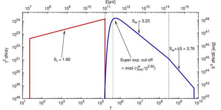
Figure 4: The two components of the electron spectrum used to calculate the broad band emission of the Crab Nebula in the constant B-field model. Red solid line: radio electrons; blue solid line: wind electrons. The black dashed lines indicate the values fot the minimum, maximum, and break energies.

Table 2: Parameters for the electron spectrum used for the constant B-field model. At the energy $\gamma_{\mathrm{min}}$ the radio electron spectrum cuts off sharply whereas the wind electrons cut off superexponentially. The energy $\gamma_{\mathrm{max}}$ denotes a sharp cut-off for the radio and wind electrons.

Parameters		Constant $B$-field model
		Radio	Wind
Normalization constant……………………. .	$\ln(N_{0})$	$120.0(1)$	$78.6(3)$
Low energy cut-off………………………….	$\ln(\gamma_{\mathrm{min}})$	$3.1$	$12.96(3)$
Super exponential cut-off parameter……………	$\beta$	–	$2.8(4)$
Break position …………………………….	$\ln(\gamma_{\mathrm{break}})$	–	$19.5(1)$
High energy cut-off…………………………	$\ln(\gamma_{\mathrm{max}})$	$12.1(7)$	$22.51(3)$
Spectral index ………………………. .	$S$	$1.60(1)$	$3.23(1)$
Spectral index (after break)…………………. .	$S+\Delta S$	–	$3.76(3)$

Table 3: Parameters for the electron spectrum for the MHD flow model. Compare Eqs. 15 and 16.

Parameters		MHD flow model
		Radio	Wind
Normalization constant……………………. .	$\ln(n_{0}),\ln(q_{0})$	$-11.41(2)$	$-1.32(1)$
Low energy cut-off………………………….	$\ln(\gamma_{\mathrm{min}})$	–	$13.94(2)$
High energy cut-off…………………………	$\ln(\gamma_{\mathrm{max}})$	$13.55(3)$	$22.60(1)$
Spectral index …………………. .	$S$	$1.58(1)$	$2.32(1)$
Magnetization parameter………………	$\sigma$	$0.0045(3)$

The radio electrons loose energy radiatively and adiabatically as the nebula expands. Interpreting the maximum Lorentz factor of the radio electrons as induced only by radiative cooling (ignoring adiabatic losses), an upper limit on the magnetic field can be derived:

$$B\leq 385\left(\frac{\gamma}{1.74\times 10^{5}}\right)^{-1/2}\left(\frac{t_{\mathrm{sy}}}{956\,\mathrm{yr}}\right)^{-1/2}\,\mu\mathrm{G}.$$ (17)

A lower limit on the magnetic field can be estimated by varying the magnetic field and the normalization $N_{0}^{r}$ of the radio electrons until the inverse Compton component overshoots the Fermi data. The constraint on the magnetic field is estimated to be $B\geq 100~{}\mu$G. The two limits are consistent with the value derived for the constant B-field model as well as with the prediction by the KC84 model.

III.2 Wind electrons

The continuously injected wind electrons produce the bulk of the observed SED above sub-mm/FIR wavelengths via synchrotron emission. The spectrum is given in Eq. 10. The radiatively cooled spectrum of the wind electrons has a spectral index of $S_{w}=3.23=2.23+1$, which can be explained naturally by 1^st-order Fermi acceleration at an ultrarelativistic shock with subsequent synchrotron cooling (see e.g. Kirk & Duffy 1999). The low-energy cut-off of the wind electrons is found to be $\gamma_{\mathrm{min}}^{w}=4.24\times 10^{5}$, which is anticipated in the model suggested by KC84. It requires the average Lorentz factor $\langle\gamma_{w}\rangle$ of the isotropized (downstream) electrons to be similar to the bulk Lorentz factor $\gamma_{*}$ of the upstream electrons, $\langle\gamma_{w}\rangle=7.33\times 10^{5}\approx\gamma_{*}$ (Kennel & Coroniti 1984; Kundt & Krotscheck 1980; Arons 1996). An additional feature present in the hard X-ray spectrum, which shows a softening at $\sim 130\,\mathrm{keV}$, corresponds to a break with $\Delta S=0.43$ at $\gamma_{\mathrm{break}}^{w}=3.01\times 10^{8}$ in the electron spectrum. The origin of this feature in the electron spectrum is very likely related to the injection/acceleration, given that it can hardly be related to energy-dependent escape. (The X-ray emitting electrons suffer cooling well before escaping the nebula.) The value of $\Delta S=0.43$ could hint at an energy dependent effect similar to diffusion in a Kolmogorov-type turbulence power spectrum.

The total energy of the radio and wind electrons, respectively, is found to be

$$E_{r} = mc^{2}\int\limits_{1}^{\infty}\,\gamma\frac{\mathrm{d}N_{\mathrm{el}}^{r}}{\mathrm{d}\gamma}\,\mathrm{d}\gamma=3.10\times 10^{48}\,\mathrm{ergs},$$ (18)

$$E_{w} = mc^{2}\int\limits_{1}^{\infty}\,\gamma\frac{\mathrm{d}N_{\mathrm{el}}^{w}}{\mathrm{d}\gamma}\,\mathrm{d}\gamma=2.28\times 10^{48}\,\mathrm{ergs},$$ (19)

indicating that the total energy in electrons is much less than the energy released through the spin-down of the pulsar. That both relic electrons and wind electrons have roughly equal energy is consistent with the expectation given by Atoyan (1999).

IV Cross calibration of IACTs & Fermi

The updated model of the SED of the Crab Nebula provides an opportunity for a cross calibration between ground-based air shower experiments and the Fermi/LAT. The method is demonstrated here with the imaging air Cherenkov telescopes HEGRA, H.E.S.S., and MAGIC but is generally applicable to any other experiment that measures the flux and spectrum from the Crab Nebula in the high-energy regime.

In general, the energy calibration of IACTs is done indirectly with the help of detailed simulations of air showers and the detector response. However, the remaining systematic uncertainty on the absolute energy scale typically of 15% leads to substantial differences in the observed flux and position of cut-offs in the energy spectra between different IACTs and also between Fermi/LAT and IACTs. First attempts to cross-calibrate the IACTs among each other have already used the Crab Nebula (Horns et al. 2005; Zechlin et al. 2008). Since the known gamma-ray spectra lack sufficient sharp features, an absolute cross calibration with lines, etc., is not feasible. So far, efforts to cross-calibrate Fermi/LAT with IACTs have focused on using the overlapping energy range (Bastieri et al. 2005). Cross calibration between Fermi/LAT and IACTs indirectly provides a means of benefiting from the careful beam-line calibration of the Fermi/LAT (see e.g. Atwood et al. 2009).

The cross calibration is accomplished in the following way (Meyer et al. 2009): The average magnetic field of the model is adapted to the Fermi observations. The statistical uncertainty on the $B$-field in Eq. 13 translates into statistical errors on this reference model (see Table 4). For each IACT an energy scaling factor $s_{\mathrm{IACT}}$ is introduced to correct the measured energy $E_{\mathrm{meas}}$ to a common energy scale $E$ such that

$$E=E_{\mathrm{meas}}\cdot s_{\mathrm{IACT}}.$$ (20)

The scaling factor $s_{\mathrm{IACT}}$ for each instrument is determined via a $\chi^{2}$-minimization in which the energy scale is changed according to the formula above until the data points reproduce the model best. The resulting scaling factors for the different instruments are listed in Table 4 with the statistical errors and the reduced minimum $\chi^{2}$-values before and after the fit. To illustrate the result, Figs. 5(a) and 5(b) compare the unscaled and the scaled data points with the model. It is evident from these figures that the scaled data points fit the model better. This is also quantified by the $\chi^{2}$-values before and after the application of the scaling factors. All scaling factors lie within the aforementioned 15% energy uncertainty of the IACTs. The complete SED with the scaled data points and the model calculations of Section II is shown in Appendix E.

The cross calibration eliminates the systematic uncertainty of the energy scale of the IACTs and adjusts them to a common one shared with the Fermi/LAT. However, the Fermi/LAT’s absolute energy uncertainty remains, but it implies an improvement from $\pm 15\%$ to $+5\%$ and $-10\%$.

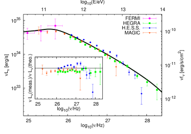
(a) The IC model (constant $B$-field model, solid black line) with measurements from IACTs and Fermi/LAT. No energy scaling is applied.

(b) The same curve as in 5(a) but with the scaling factors of Eq. 20 and Table 4 applied to the data.

Figure 5: Comparison between the unscaled and scaled data of the IACTs.

Instrument	Scaling factor $s_{\mathrm{IACT}}$	Stat. error $\Delta s$	$\chi^{2}_{\mathrm{before}}/\mathrm{d.o.f.}$	$\chi^{2}_{\mathrm{after}}/\mathrm{d.o.f.}$
Fermi/LAT	$1$	$+0.05~{}-0.03$	–	$0.49$
HEGRA	$1.042$	$\pm 0.005$	$7.652$	$1.046$
H.E.S.S.	$0.961$	$\pm 0.004$	$11.84$	$6.476$
MAGIC	$1.03$	$\pm 0.01$	$1.671$	$0.656$

Table 4: Energy scaling factors of the IACTs for the cross calibration.

As a first application of the cross calibration, we derive upper limits on the diffuse $\gamma$-ray background. Both Fermi (Abdo et al. 2009) and H.E.S.S. (Aharonian et al. 2008, 2009) have measured the cosmic ray $e^{-}+e^{+}$ spectrum. Unlike Fermi/LAT, the telescopes from H.E.S.S. cannot accurately distinguish between showers induced by electrons (or positrons) or photons, such that up to $\approx 50$% of the observed electromagnetic air showers could be induced by photons. Therefore, H.E.S.S. actually measures electrons and diffuse background photons. Taking the difference of the two measurements we can derive an upper limit on the intensity of the $\gamma$-ray background. The scaling factors derived above are now used to convert the H.E.S.S. data to the Fermi/LAT energy scale, which substantially reduces the systematic uncertainty on the observed intensity, given that the electron spectrum follows a soft power law with $\propto E^{-3}$. An important result of the cross calibration is that the peak in the spectrum observed by ATIC (Chang et al. 2008) appears more unlikely after applying the scaling factors.

The upper limits are derived by taking the difference of the two measurements from the energy region covered by both instruments. This corresponds to the first six H.E.S.S. points of the low energy analysis in Fig. 6. The remaining systematic errors are taken into account for deriving the upper limits: the flux points of the H.E.S.S. measurements are shifted to their maximum value allowed by the systematic uncertainties while the Fermi points are shifted to the minimum value. This gives a conservative approximation for the upper limits. In general, the scaling factors can be used, e.g., to improve contraints on dark matter model parameters that rely on combined measurements (see e.g. Kistler & Siegal-Gaskins 2010).

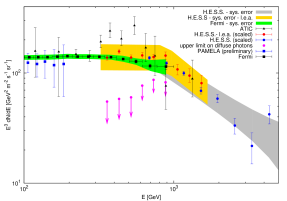
Figure 6: $e^{-}+e^{+}$ spectrum reported by H.E.S.S. and Fermi. The cross calibration factor is applied to the H.E.S.S. energy scale, so the uncertainty on the global energy scale is reduced. The abbreviation l.e.a. stands for low-energy analysis as applied to the H.E.S.S. data in Aharonian et al. (2009). For comparison, the PAMELA data points are taken from Mocchiutti et al. (2010).

V Summary

Updated models and data compilation for the SED of the Crab Nebula have been presented. The MHD flow model based upon KC84 and AA96 does not provide a satisfactory description of the available data and requires refinements of the underlying assumptions, e.g., relaxing spherical symmetry in axisymmetric numerical calculations as carried out by Volpi et al. (2008). A straightforward modification is, among others, the introduction of an anisotropic wind with variations of $\sigma$ when moving out of the equatorial plane towards the polar regions of the outflow. The simplified approach of a constant magnetic field pursued here has the benefit of a smaller total number of parameters, even though the prescription of the injection spectrum in the MHD model is simpler (7 instead of 10 parameters) and physically more meaningful. Most important for the task of cross-calibrating the instruments, the inverse Compton component predicted in this model accurately describes all observational data above $1$ GeV for a magnetic field of $B=\left(124\,{}\pm 6\,\mathrm{(stat.)}\,{}^{+15}_{-6}\,\mathrm{(sys.)}\right)\,\mu\mathrm{G}$. The comprehensive SED allows for an estimate of the dust mass. In contrast to Temim et al. (2006), we obtain a value about 40% lower, namely $M_{\mathrm{dust}}=4\times 10^{-4}M_{\odot}$. The radio (relic) electrons provide additional (independent) constraints on the average magnetic field in the entire radio nebula. Using the endpoint of the electron spectrum the magnetic field is constrained to be smaller than $\approx 385~{}\mu$G, while the Fermi/LAT observations set a lower limit at approx. $100~{}\mu$G.

The model describes the broad band data at high energies well enough to derive energy scaling factors for cross-calibrating the Fermi/LAT instrument with a variety of ground-based instruments. The cross-calibration eliminates the systematic uncertainty of the different energy scales used by the IACTs and ultimately reduces the global uncertainty to the Fermi/LAT calibration uncertainties of $+5$% and $-10$%. An application of the cross calibration were presented, and upper limits on the diffuse photon background between 200 GeV and 1 TeV derived by combining Fermi/LAT with H.E.S.S. measurements. The excess measured by the ATIC collaboration seems unlikely with the scaled H.E.S.S. observations.
The presented cross calibration can be used universally when combining observational data from various instruments, as well as in cases where the absolute energy scale is important. Specifically for soft spectra with cut-off features, such as in observations of objects at cosmological distances suffering from absorption on the extragalactic background light, the cross calibration can be useful for providing more stringent upper limits.

Appendix A Spatial distribution of seed photons and electrons in the nebula

To calculate the seed photon fields required to calculate the IC flux, it is neccessary to convert the observed photon flux to the corresponding photon densities. This is done by following the approach suggested by Hillas et al. (1998). Both the photon densities (apart from the CMB contribution) and electron density are assumed to follow Gaussian densities in the distance $r$ from the Nebula’s center, $\exp[-r^{2}/(2\sigma^{2})]$ and $\exp[-r^{2}/(2\rho^{2})]$, respectively. The variances $\sigma^{2}$ and $\rho^{2}$ are energy dependent and estimated from observations. For the Gaussian describing the photon density Hillas et al. (1998) find

$$\arctan\left(\frac{\sigma}{d}\right)=$$

$$\left\{\begin{array}[]{ll}3.93\times 10^{-4}&\mathrm{for}\,\epsilon<0.02\,\mathrm{eV},\\ \\ \left(0.47+3.46\left[\frac{\epsilon}{0.02\,\mathrm{eV}}\right]^{-0.09}\right)\times 10^{-4}&\mathrm{for}\,\epsilon\geq 0.02\,\mathrm{eV}.\end{array}\right.$$ (24)

Assuming that the photons are produced only via synchrotron radiation in a uniform magnetic field, the variance of the electron density follows directly from Eq. 35 with the aforementioned averaging over $\theta$,

$$\arctan\left(\frac{\rho}{d}\right)=$$

$$\left\{\begin{array}[]{ll}3.93\times 10^{-4}&\mathrm{for}\,\gamma<6.65\times 10^{4}\\ \\ \left(0.47+28.9~{}\gamma^{-0.17}\left[\frac{B}{10^{-4}\,\mathrm{G}}\right]^{-0.09}\right)\times 10^{-4}&\mathrm{for}\,\gamma\geq 6.65\times 10^{4}.\\ \end{array}\right.$$ (28)

Only those photons and electrons with overlapping distributions can interact, so that the total distribution is found by convolution to give a total variance of $\sigma^{2}+\rho^{2}$. For a photon production rate $S_{\nu}$, which is the sum of the contributions from synchrotron radiation, thermal dust emission, and optical line emission, we find

$$n_{\mathrm{Seed}}=\frac{S_{\nu}}{4\pi c(\rho^{2}+\sigma^{2})}+n_{\mathrm{CMB}}.$$ (30)

The photon production rates are calculated using the individual luminosities, $S_{\nu}=L_{\nu}/(h\nu)$, where

$$L_{\nu}^{\mathrm{sync}} = \int\limits_{1}^{\infty}\frac{\mathrm{d}N_{\mathrm{el}}}{\mathrm{d}\gamma}\mathcal{L}_{\nu}^{\mathrm{Sy}}\mathrm{d}\gamma,$$ (31)

$$L_{\nu}^{\mathrm{opt}} = \sum_{i}L_{i}^{\mathrm{opt}}\delta(\nu-\nu_{i}).$$ (32)

The fluxes from the line emissions are approximated by $\delta$-distributions, and the $L_{i}$ are given in the references, see Section II. The luminosity for the dust emission is given by a gray body spectrum and the photon density of the CMB is calculated from a black body with a temperature of $T=2.726$ K. The total seed photon field can then be used to calculate the inverse Compton emissions by means of Eqs. 34 and 12.

Appendix B Single-particle emission functions

The single-particle emission functions for particles of mass $m$ and energy $\gamma mc^{2}$ for synchrotron $\mathcal{L}_{\nu}^{\mathrm{Sy}}$ and inverse Compton emission $\mathcal{L}_{\nu}^{\mathrm{IC}}$ used in Eq. 12 are taken from Blumenthal & Gould (1970):

$$\mathcal{L}_{\nu}^{\mathrm{Sy}} = \frac{\sqrt{3}e^{3}B\sin\theta}{mc^{2}}~{}\frac{\nu}{\nu_{\mathrm{c}}}\int\limits_{\nu/\nu_{\mathrm{c}}}^{~{}\infty}K_{5/3}(x)~{}\mathrm{d}x\,,$$ (33)

$$\mathcal{L}_{\nu}^{\mathrm{IC}} = \frac{3}{4}~{}\frac{\sigma_{\mathrm{T}}c}{\gamma^{2}}h\nu\int\limits_{h\nu/(4\gamma^{2})}^{~{}h\nu}~{}\mathrm{d}\epsilon~{}\frac{n_{\mathrm{seed}}(\epsilon)}{\epsilon}f_{\mathrm{IC}}(\epsilon,\nu,\gamma).$$ (34)

We denote the photon energy after scattering by $h\nu$ and before scattering by $\epsilon$, the Thomson cross section by $\sigma_{\mathrm{T}}$ and the electron charge by $e$. The critical frequency $\nu_{\mathrm{c}}$ is defined as

$$\nu_{\mathrm{c}}=\frac{3e}{4\pi mc}~{}B\sin\theta~{}\gamma^{2},$$ (35)

and $K_{5/3}(x)$ stands for the modified Bessel function of fractional order $5/3$. The electron pitch angle $\theta$ is averaged where the value $\langle\sin\theta\rangle=\sqrt{2/3}$ is adopted. Introducing the kinematic variable $q$,

$$q=\frac{h\nu}{4\epsilon\gamma^{2}[1-h\nu/(\gamma mc^{2})]},$$ (36)

the IC distribution function $f_{\mathrm{IC}}$ can be written as

$$f_{\mathrm{IC}}(\epsilon,\nu,\gamma) =$$

$$2q\ln q + (1+2q)(1-q)+\frac{1}{2}~{}\frac{\left[{4\epsilon\gamma q}/{\left(mc^{2}\right)}\right]^{2}}{1+{4\epsilon\gamma q}/{\left(mc^{2}\right)}}(1-q).$$ (37)

Appendix C Correlation between the fit parameters

The covariance matrix has been calculated at the position of the minimum in the $\chi^{2}$-function. The diagonal elements of the covariance matrix have been already listed in the form of estimates of the error of the individual parameters, see Tables 2 and 3. Here, we list the correlation matrix defined as $\mathrm{cor}(i,j)=\sqrt{\mathrm{cov}(i,j)/(\sigma_{i}\sigma_{j})}$ in Table 5 for the constant $B$-field model and in Table 6 for the MHD flow model.

Table 5: The correlation coefficients between the fit-parameters for the constant B-field model. Since the matrix is symmetric, the lower trigonal part is not listed.

	$S_{r}$	$\ln(N_{0}^{r})$	$\ln(\gamma^{r}_{\mathrm{max}})$	$\ln(\gamma^{w}_{\mathrm{min}})$	$\ln(\gamma^{w}_{\mathrm{break}})$	$\ln(\gamma^{w}_{\mathrm{max}})$	$\beta$	$S_{w}$	$S_{w}+\Delta S$	$\ln(N_{0}^{w})$
$S_{r}$	1	$-1.00$	$-0.35$	$-0.02$	$-0.03$	$-0.02$	$0.10$	$0.05$	$0.02$	$0.03$
$\ln(N_{0}^{r})$		1	$0.34$	$0.02$	$0.03$	$0.02$	$-0.10$	$-0.05$	$-0.01$	$-0.03$
$\ln(\gamma^{r}_{\mathrm{max}})$			1	$0.24$	$-0.05$	$-0.03$	$0.26$	$0.08$	$0.02$	$0.05$
$\ln(\gamma^{w}_{\mathrm{min}})$				1	$0.56$	$0.13$	$-0.57$	$-0.80$	$-0.25$	$-0.57$
$\ln(\gamma^{w}_{\mathrm{break}})$					1	$0.39$	$-0.46$	$-0.82$	$-0.70$	$-1.00$
$\ln(\gamma^{w}_{\mathrm{max}})$						1	$-0.11$	$-0.22$	$-0.75$	$-0.38$
$\beta$							1	$0.71$	$0.19$	$0.47$
$S_{w}$								1	$0.42$	$0.84$
$S_{w}+\Delta S$									1	$0.69$
$\ln(N_{0}^{w})$										1

Table 6: The correlation coefficients between the fit-parameters for the MHD flow model. Since the matrix is symmetric, the lower trigonal part is not listed.

	$\ln(q_{0})$	$\ln(n_{0})$	$\ln(\gamma^{r}_{\mathrm{max}})$	$\ln(\gamma^{w}_{\mathrm{min}})$	$\ln(\gamma^{w}_{\mathrm{max}})$	$S_{w}$	$S_{r}$
$\ln(q_{0})$	1	$-0.02$	$0.23$	$0.79$	$0.94$	$-0.00$	$0.00$
$\ln(n_{0})$		1	$-0.50$	$-0.03$	$-0.02$	$-0.01$	$0.01$
$\ln(\gamma^{r}_{\mathrm{max}})$			1	$0.31$	$0.19$	$0.01$	$-0.01$
$\ln(\gamma^{w}_{\mathrm{min}})$				1	$0.65$	$0.01$	$-0.01$
$\ln(\gamma^{w}_{\mathrm{max}})$					1	$-0.11$	$0.11$
$S_{w}$						1	$-1.00$
$S_{r}$							1

Appendix D Parametrization of IC flux

For convenience, the energy flux $\nu f_{\nu}$ of the IC emission for $1$ GeV $<E<1$ PeV is parametrized as a function of energy, namely a 5^th-order polynomial in double-logarithmic representation (as done by Aharonian et al. 2004):

$$\log_{10}\left(\frac{\nu f_{\nu}}{\,\mathrm{erg}\,\mathrm{s}^{-1}\,\mathrm{cm}^{-2}}\right)=\sum_{i=0}^{5}p_{i}\log_{10}^{i}\left(\frac{E}{\,\mathrm{TeV}}\right).$$ (38)

The coefficients are given in Table 7. The relative error of the parametrization for the parameters $p_{3}$ and $p_{5}$ are approximately 6%, less than 1% for $p_{0}$ and $p_{2}$ and about 1% for $p_{1}$. The value of $p_{4}$ is set to zero since its relative error is otherwise around 150%, and thus $p_{4}$ is not neccessary for a satisfactory fit.

Table 7: Parametrization of the IC flux. The coefficients correspond to Eq. 38.

Coefficient	Value
$p_{0}$ ……………………	$-10.2708$
$p_{1}$ ……………………	$-0.53616$
$p_{2}$ ……………………	$-0.179475$
$p_{3}$ ……………………	$0.0473174$
$p_{4}$ ……………………	$0$
$p_{5}$ ……………………	$-0.00449161$

Appendix E Final SED

Figure 7 summarizes the best fits for the constant B-field model and the MHD flow model (see Section II), together with all data points of the references in Table 1 and in Aharonian et al. (2004). Likewise, the scaling factors for the IACTs introduced in Section IV are also applied.

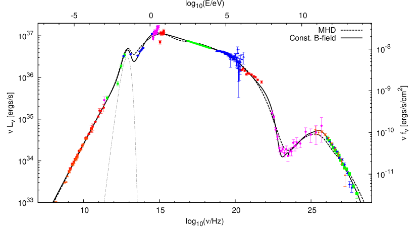
Figure 7: The SED with the best-fitting model calculations.