Spin-flavor oscillations of Dirac neutrinos described by relativistic quantum mechanics

Abstract

Spin-flavor oscillations of Dirac neutrinos in matter and a magnetic field are studied using the method of relativistic quantum mechanics. Using the exact solution of the wave equation for a massive neutrino, taking into account external fields, the effective Hamiltonian governing neutrino spin-flavor oscillations is derived. Then the The consistency of our approach with the commonly used quantum mechanical method is demonstrated. The obtained correction to the usual effective Hamiltonian results in the appearance of the new resonance in neutrino oscillations. Applications to spin-flavor neutrino oscillations in an expanding envelope of a supernova are discussed. In particular, transitions between right-polarized electron neutrinos and additional sterile neutrinos are studied for realistic background matter and magnetic field distributions. The influence of other factors such as the longitudinal magnetic field, the matter polarization, and the non-standard contributions to the neutrino effective potential, is also analyzed.

I Introduction

It was confirmed by numerous experiments that neutrinos are massive particles and there is a mixing between different neutrino generations. Besides these non-standard model neutrino properties it is believed that neutrinos can also have non-zero diagonal and transition magnetic moments. The latter mix both eigenstates with opposite helicities as well as different neutrino flavors. Thus the existence of transition magnetic moments implies that in presence of an external electromagnetic field conversions of left-handed neutrinos into their right-handed counterparts of another flavor (neutrino spin-flavor oscillations VolVysOku86 ; LimMar88 ) are possible, $\nu_{\alpha}^{\mathrm{-{}}}\leftrightarrow\nu_{\beta}^{\mathrm{+{}}}$, where $\alpha\neq\beta$ and the index $\pm{}$ corresponds to different neutrino helicities.

In this work we will consider spin-flavor oscillations of Dirac neutrinos in dense matter under the influence of strong external magnetic fields. Although the existence of Majorana neutrinos is favored in various neutrino mass generation models, like see-saw mechanism FukYan03p391 , the question whether neutrinos are Dirac or Majorana particles is still open AviEllEng08 .

Note that Dirac and Majorana neutrinos have completely different structure of the magnetic moments matrix. Dirac neutrinos can have both diagonal and transition magnetic moments whereas Majorana neutrinos only transition ones (see, e.g., Ref. FukYan03p461 ). Moreover the magnetic moments matrix is symmetric in the Dirac case and anti-symmetric for Majorana neutrinos FukYan03p461 .

The strongest laboratory constraint on the neutrino effective magnetic moment, obtained by the GEMMA collaboration nuMMexp , is $3.2\times 10^{-11}\mu_{\mathrm{B}}$, where $\mu_{\mathrm{B}}$ is the Bohr magneton. Slightly weaker upper bound on the magnetic moments of neutrinos was obtained by the BOREXINO collaboration Arp08 . Note that the astrophysical limits on the magnetic moments of Dirac and Majorana neutrinos extracted from the white dwarfs cooling rate Raf99 can be even stronger than the laboratory ones. Therefore in most realistic situations, where the magnetic field is not too strong, neutrino spin and spin-flavor oscillations are likely to play a sub-leading role AkhPul03 . Nevertheless in some astrophysical media the dynamics of neutrino oscillations can be significantly affected by a magnetic field because of its interaction with neutrino magnetic moments. For example, during a supernova explosion or in the vicinity of a neutron star, magnetic fields can reach values up to $10^{16}\thinspace\mathrm{G}$ Aki03 , which is enough to influence the neutrino oscillations process in a significant way.

Neutrino spin and spin-flavor oscillations in a supernova were discussed in Refs. LimMar88 ; Vol88 . The impact of neutrino magnetic moments and spin-flavor oscillations on $r$-process nucleosynthesis during a supernova explosion was studied in Ref. BalVolWel07 . The neutrino spin flip, i.e. the transformation like $\nu_{\alpha}^{\mathrm{-{}}}\leftrightarrow\nu_{\alpha}^{\mathrm{+{}}}$ within the same flavor, can happen not only because of the magnetic moment interaction with an external magnetic field, but also in collisions with background matter during a supernova explosion, that was examined in Ref. Not88 .

In this work we study neutrino spin-flavor oscillations in frames of the relativistic quantum mechanics Dvo ; Dvo06 ; DvoMaa07 ; Dvo08JPCS ; Dvo08JPG . Within the developed formalism we find the wave functions of neutrino mass eigenstates, which are the superposition of flavor neutrinos, for a given initial condition (Sec. II). Using this method for the description of the neutrino evolution one can exactly take into account neutrino masses and the influence of external fields since we use exact solutions of the Dirac equation for massive Dirac neutrinos. Note that neutrino oscillations in dense matter and strong magnetic fields can be also described with help of the methods of finite temperature field theory NotRaf88 .

Then, in Sec. III, we analyze the conventional quantum mechanical approach to the description of neutrino spin-flavor oscillations LimMar88 . We discuss the cases of the neutrino propagation in dense matter and weak magnetic field and in low density matter and strong magnetic field. Then we demonstrate that the relativistic quantum mechanics approach is consistent with the previously used formalism and obtain the corrections to the standard effective Hamiltonian. We show that the correction obtained results in the appearance of the new resonance in neutrino oscillations.

In Sec. IV we discuss a possible application of our results to the conversion of right-handed electron neutrinos, which can be created in a supernova explosion Not88 , into a quasi-degenerate in mass sterile neutrino when particles propagate in an expanding envelope of a supernova and interact with its magnetic field. The importance of other factors, which can also influence the neutrino oscillations process, is considered in Sec. V. Finally, in Sec. VI, we summarize our results.

II Relativistic quantum mechanics description

Let us study the time evolution of the system of two mixed flavor neutrinos $(\nu_{\alpha},\nu_{\beta})$ in matter and in an external electromagnetic field $F_{\mu\nu}=(\mathbf{E},\mathbf{B})$. The indexes $\alpha$ and $\beta$ can stand for any of the neutrino flavors $e$, $\mu$ or $\tau$. The interaction with background matter can be represented in terms of the external axial vector fields $f^{\mu}_{\lambda\lambda^{\prime}}$. The Lagrangian for our system has the form,

$$\mathcal{L}= \sum_{\lambda=\alpha,\beta}\bar{\nu}_{\lambda}\mathrm{i}\gamma^{\mu}\partial_{\mu}\nu_{\lambda}-\sum_{\lambda\lambda^{\prime}=\alpha,\beta}\bar{\nu}_{\lambda}\Big{(}m_{\lambda\lambda^{\prime}}+\gamma_{\mu}^{\mathrm{L}}f^{\mu}_{\lambda\lambda^{\prime}}$$

$$+\frac{1}{2}M_{\lambda\lambda^{\prime}}\sigma_{\mu\nu}F^{\mu\nu}\Big{)}\nu_{\lambda^{\prime}},$$ (1)

where $(m_{\lambda\lambda^{\prime}})$ is the nondiagonal mass matrix and $(M_{\lambda\lambda^{\prime}})$ is the matrix of the neutrino magnetic moments. Note that in general case the matrices $(m_{\lambda\lambda^{\prime}})$ and $(M_{\lambda\lambda^{\prime}})$ are independent, i.e. the diagonal form of the matrix $(m_{\lambda\lambda^{\prime}})$ in a certain basis does not imply that of the matrix $(M_{\lambda\lambda^{\prime}})$.

In the case of the standard model neutrino interactions the matrix $(f^{\mu}_{\lambda\lambda^{\prime}})$ is diagonal: $f^{\mu}_{\lambda\lambda^{\prime}}=f^{\mu}_{\lambda}\delta_{\lambda\lambda^{\prime}}$, where $f^{\mu}_{\lambda}=(f^{0}_{\lambda},\mathbf{f}_{\lambda})$. The possible nondiagonal elements of the matrix $f^{\mu}_{\lambda\lambda^{\prime}}$, with $\lambda\neq\lambda^{\prime}$, correspond to the non-standard neutrino interactions with matter Dvo08JPCS . In the following we will study neutrino oscillations in non-moving and unpolarized matter with $\mathbf{f}_{\lambda}=0$. The explicit form of the zero-th component $f^{0}_{\lambda}\equiv f_{\lambda}$ of the four vector $f^{\mu}_{\lambda}$ for the electoneutral medium consisting of electrons, protons and neutrons can be found in Ref. DvoStu02 . In the case of sterile neutrinos $f_{\nu_{s}}=0$.

To study the time evolution of the system (II) it is necessary to formulate the initial condition for the flavor neutrinos $\nu_{\lambda}$. We suppose that only one neutrino flavor, e.g., “$\beta$”, is present initially (see Refs. Dvo ; Dvo06 ; DvoMaa07 ; Dvo08JPCS ; Dvo08JPG ), i.e. $\nu_{\alpha}(\mathbf{r},0)=0$, and $\nu_{\beta}(\mathbf{r},0)=\nu_{\beta}^{(0)}(\mathbf{r})$, where $\nu_{\beta}^{(0)}(\mathbf{r})$ is the given function. Then we will look for the wave function $\nu_{\alpha}$ at $t>0$. If we choose $\alpha=\mu$ or $\tau$ and $\beta=e$, it will correspond to the typical situation of neutrinos emitted in the Sun: for the given initial flux of electron neutrinos we study the presence of other neutrino flavors at subsequent moments of time. Note that the analogous initial condition problem for neutrino wave packets was studied in Ref. BerLeo04 .

To analytically study the Dirac equation in presence of external fields we will consider the case of the coordinate independent functions $f_{\lambda}$ and $F_{\mu\nu}$. The analysis of the validity of this approximation will be made in Sec. V. For the coordinate independent external fields the momentum of the particles $\mathbf{p}$ is conserved.

Moreover, the additional constraint can be imposed on the wave function $\nu_{\beta}^{(0)}(\mathbf{r})$,

$$P_{\pm{}}\nu_{\beta}^{(0)}(\mathbf{r})=\nu_{\beta}^{(0)}(\mathbf{r}),\quad P_{\pm{}}=\left(1\pm\frac{(\bm{\Sigma}\cdot\mathbf{p})}{|\mathbf{p}|}\right),$$ (2)

where $\bm{\Sigma}=-\gamma^{0}\gamma^{5}\bm{\gamma}$ are the Dirac matrices. Eq. (2) implies that initially neutrinos of the flavor “$\beta$” have a certain helicity. If we act with the operator $P_{\mp{}}$ on the final state $\nu_{\alpha}(\mathbf{r},t)$, we can study the appearance of the opposite helicity eigenstates among neutrinos of the flavor “$\alpha$”, i.e this situation corresponds to the neutrino spin flavor oscillations $\nu_{\beta}^{\mathrm{L,R}}\leftrightarrow\nu_{\alpha}^{\mathrm{R,L}}$.

Note that, unlike the helicity states defined in Eq. (2), the chirality of a particle is a eigenvalue of the matrix $\gamma^{5}$: $\gamma^{5}\psi=\varkappa\psi$. In case of massive Dirac particles the helicity and the chirality do not coincide Zub04 . The helicity is a conserving number whereas the chirality – not, since the operator $\gamma^{5}$ does not commute with a Hamiltonian.

Let us introduce the neutrino mass eigenstates $\psi_{a}$, $a=1,2$, as

$$\nu_{\lambda}=\sum_{a=1,2}U_{\lambda a}\psi_{a},\quad(U_{\lambda a})=\begin{pmatrix}\cos\theta&-\sin\theta\\ \sin\theta&\cos\theta\ \end{pmatrix},$$ (3)

to diagonalize the mass matrix $(m_{\lambda\lambda^{\prime}})$. In Eq. (3) we take into account that for the two neutrinos system the mixing matrix $(U_{\lambda a})$ can be parameterized with help of one vacuum mixing angle $\theta$. We suppose that the mass eigenstates $\psi_{a}$ are Dirac particles with the masses $m_{a}$.

The Lagrangian (II) expressed in terms of the fields $\psi_{a}$ takes the form,

$$\mathcal{L}= \sum_{a=1,2}\bar{\psi}_{a}(\mathrm{i}\gamma^{\mu}\partial_{\mu}-m_{a})\psi_{a}$$

$$-\sum_{ab=1,2}\bar{\psi}_{a}\left(\gamma_{\mu}^{\mathrm{L}}g^{\mu}_{ab}+\frac{1}{2}\mu_{ab}\sigma_{\mu\nu}F^{\mu\nu}\right)\psi_{b},$$ (4)

where

$$(\mu_{ab})= U^{\dagger}(M_{\lambda\lambda^{\prime}})U=\begin{pmatrix}\mu_{1}&\mu\\ \mu&\mu_{2}\ \end{pmatrix},$$

$$(g_{ab})= U^{\dagger}(f_{\lambda\lambda^{\prime}})U=\begin{pmatrix}g_{1}&g\\ g&g_{2}\ \end{pmatrix},$$ (5)

are the nondiagonal matrices of neutrino magnetic moments and neutrino interaction with matter in the mass eigenstates basis. In Eq. (II) we take into account that background matter is non-moving and unpolarized, i.e. only the zero-th component $g_{ab}\equiv g_{ab}^{0}$ of the four vector $g_{ab}^{\mu}$ survives.

To discuss the time evolution of the system (II) we write down the wave equations which result from Eq. (II),

$$\mathrm{i}\dot{\psi}_{a}= \mathcal{H}_{a}\psi_{a}+V\psi_{b},\quad a=1,2,\quad a\neq b,$$

$$\mathcal{H}_{a}= (\bm{\alpha}\mathbf{p})+\beta m_{a}-\mu_{a}\beta\Sigma_{3}B+g_{a}(1-\gamma^{5})/2,$$

$$V= -\mu\beta\Sigma_{3}B+g(1-\gamma^{5})/2,$$ (6)

where $\alpha=\gamma^{0}\bm{\gamma}$ and $\beta=\gamma^{0}$ are the Dirac matrices. Here we study the neutrino motion along the $x$-axis: $\mathbf{p}=(p,0,0)$, in only transversal magnetic field: $\mathbf{B}=(0,0,B)$ and $\mathbf{E}=0$.

Note that we cannot directly solve the wave equations (II) because of the nondiagonal interaction $V$ which mixes different mass eigenstates. In vacuum, i.e in the absence of external fields, when $(g_{ab}^{\mu})=0$ and $F_{\mu\nu}=0$, the mass eigenstates $\psi_{1,2}$ decouple and the system (II) can be easily solved. Nevertheless we can point out an exact solution of the wave equation $\mathrm{i}\dot{\psi}_{a}=\mathcal{H}_{a}\psi_{a}$, for a single mass eigenstate $\psi_{a}$, that exactly accounts for the influence of the external fields.

We look for the solution of Eq. (II) in the following form Dvo ; Dvo06 ; DvoMaa07 ; Dvo08JPCS ; Dvo08JPG :

$$\psi_{a}(\mathbf{r},t)= e^{-\mathrm{i}g_{a}t/2}\int\frac{\mathrm{d}^{3}\mathbf{p}}{(2\pi)^{3/2}}e^{\mathrm{i}\mathbf{p}\mathbf{r}}$$

$$\times\sum_{\zeta=\pm 1}\Big{[}a_{a}^{(\zeta)}(t)u_{a}^{(\zeta)}\exp{(-\mathrm{i}E_{a}^{(\zeta)}t)}$$

$$+b_{a}^{(\zeta)}(t)v_{a}^{(\zeta)}\exp{(\mathrm{i}E_{a}^{(\zeta)}t)}\Big{]},$$ (7)

where the energy levels, which were found in Ref. Dvo08JPG , have the form,

$$E^{(\zeta)}_{a}=\sqrt{\mathcal{M}^{2}_{a}+m^{2}_{a}+p^{2}-2\zeta R^{2}_{a}},$$ (8)

where $R^{2}_{a}=\sqrt{p^{2}\mathcal{M}^{2}_{a}+(\mu_{a}B)^{2}m^{2}_{a}}$ and $\mathcal{M}_{a}=\sqrt{(\mu_{a}B)^{2}+g_{a}^{2}/4}$. The basis spinors can be found in the limit of a small neutrino mass Dvo08JPG ,

$$u^{(\zeta)}_{a}= \frac{1}{2\sqrt{2\mathcal{M}_{a}(\mathcal{M}_{a}-\zeta g_{a}/2)}}\begin{pmatrix}\mu_{a}B+\zeta\mathcal{M}_{a}-g_{a}/2\\ \mu_{a}B-\zeta\mathcal{M}_{a}+g_{a}/2\\ \mu_{a}B-\zeta\mathcal{M}_{a}+g_{a}/2\\ \mu_{a}B+\zeta\mathcal{M}_{a}-g_{a}/2\ \end{pmatrix},$$

$$v^{(\zeta)}_{a}= \frac{1}{2\sqrt{2\mathcal{M}_{a}(\mathcal{M}_{a}+\zeta g_{a}/2)}}\begin{pmatrix}\mathcal{M}_{a}-\zeta[\mu_{a}B-g_{a}/2]\\ \mathcal{M}_{a}+\zeta[\mu_{a}B+g_{a}/2]\\ -\mathcal{M}_{a}-\zeta[\mu_{a}B+g_{a}/2]\\ -\mathcal{M}_{a}+\zeta[\mu_{a}B-g_{a}/2]\ \end{pmatrix}.$$ (9)

It should be noted that the discrete quantum number $\zeta=\pm 1$ in Eqs. (II)-(II) does not correspond to the helicity quantum states.

Now our goal is to find the time dependent coefficients $a_{a}^{(\zeta)}(t)$ and $b_{a}^{(\zeta)}(t)$. In the case of neutrino propagation in vacuum these coefficients do not depend on time and their values are completely defined by the initial condition. If we put the ansatz (II) in the wave equations (II), we get the following ordinary differential equations for the function $a_{a}^{(\zeta)}(t)$:

$$\mathrm{i}\dot{a}_{a}^{(\zeta)}=e^{\mathrm{i}(g_{a}-g_{b})t/2}\exp\left(\mathrm{i}E_{a}^{(\zeta)}t\right)u^{(\zeta){\dagger}}_{a}V\sum_{\zeta^{\prime}=\pm 1}\left[a_{b}^{(\zeta^{\prime})}u^{(\zeta^{\prime})}_{b}\exp\left(-\mathrm{i}E_{b}^{(\zeta^{\prime})}t\right)+b_{b}^{(\zeta^{\prime})}v^{(\zeta^{\prime})}_{b}\exp\left(\mathrm{i}E_{b}^{(\zeta^{\prime})}t\right)\right].$$ (10)

To obtain Eq. (10) we use the orthonormality of the basis spinors (II). Note that the differential equation for the function $b_{a}^{(\zeta)}$ is analogous to Eq. (10) and thus omitted. Moreover, taking into account the fact that $\langle u^{(\zeta)}_{a}|V|v^{(\zeta^{\prime})}_{b}\rangle=0$, we get that the equations for $a_{a}^{(\zeta)}(t)$ and $b_{a}^{(\zeta)}(t)$ decouple, i.e. the interaction $V$ does not mix positive and negative energy eigenstates.

Let us rewrite Eq. (10) in the more conventional effective Hamiltonian form. For this purpose we introduce the “wave function” $\Psi^{{}^{\prime}\mathrm{T}}=(a_{1}^{-{}},a_{2}^{-{}},a_{1}^{+{}},a_{2}^{+{}})$. Directly from Eq. (10) we derive the equation for $\Psi^{\prime}$,

$$\mathrm{i}\frac{\mathrm{d}\Psi^{\prime}}{\mathrm{d}t}=H^{\prime}\Psi^{\prime},\quad H^{\prime}=\begin{pmatrix}0&h_{-{}}e^{\mathrm{i}\omega_{-{}}t}&0&H_{-{}}e^{\mathrm{i}\Omega_{-{}}t}\\ h_{-{}}e^{-\mathrm{i}\omega_{-{}}t}&0&H_{+{}}e^{-\mathrm{i}\Omega_{+{}}t}&0\\ 0&H_{+{}}e^{\mathrm{i}\Omega_{+{}}t}&0&h_{+{}}e^{\mathrm{i}\omega_{+{}}t}\\ H_{-{}}e^{-\mathrm{i}\Omega_{-{}}t}&0&h_{+{}}e^{-\mathrm{i}\omega_{+{}}t}&0\ \end{pmatrix},$$ (11)

where $h_{\pm{}}=\langle u^{\pm{}}_{a}|V|u^{\pm{}}_{b}\rangle$, $H_{\pm{}}=\langle u^{\pm{}}_{1}|V|u^{\mp{}}_{2}\rangle$, $\omega_{\mp{}}=E_{1}^{\mp{}}-E_{2}^{\mp{}}+(g_{1}-g_{2})/2$, and $\Omega_{\mp{}}=E_{1}^{\mp{}}-E_{2}^{\pm{}}+(g_{1}-g_{2})/2$. Note that we do not give here the explicit form of the scalar products $h_{\pm{}}$ and $H_{\pm{}}$ in order not to encumber the text.

Instead of $\Psi^{\prime}$ it is more convenient to use the transformed “wave function” $\Psi$ defined by $\Psi^{\prime}=\mathcal{U}\Psi$, where $\mathcal{U}=\mathrm{diag}\left\{e^{\mathrm{i}(\Omega+\omega_{-{}})t/2},e^{\mathrm{i}(\Omega-\omega_{-{}})t/2},e^{-\mathrm{i}(\Omega-\omega_{+{}})t/2},e^{-\mathrm{i}(\Omega+\omega_{+{}})t/2}\right\}$ and $\Omega=(\Omega_{-{}}-\Omega_{+{}})/2$. Using the property $\omega_{+{}}+\omega_{-{}}=\Omega_{+{}}+\Omega_{-{}}$, we arrive to the new Schrödinger equation for the “wave function” $\Psi$,

$$\mathrm{i}\frac{\mathrm{d}\Psi}{\mathrm{d}t}=H\Psi,\quad H=\mathcal{U}^{\dagger}H^{\prime}\mathcal{U}-\mathrm{i}\mathcal{U}^{\dagger}\dot{\mathcal{U}}=\begin{pmatrix}(\Omega+\omega_{-{}})/2&h_{-{}}&0&H_{-{}}\\ h_{-{}}&(\Omega-\omega_{-{}})/2&H_{+{}}&0\\ 0&H_{+{}}&-(\Omega-\omega_{+{}})/2&h_{+{}}\\ H_{-{}}&0&h_{+{}}&-(\Omega+\omega_{+{}})/2\ \end{pmatrix}.$$ (12)

Despite initially we used the analog of the perturbation theory to analyze the influence of the potential $V$ on the dynamics of the system (II), the contribution of this potential is exactly taken into account in Eq. (12).

As we mentioned above, the quantum number $\zeta$ does not correspond to a definite helicity eigenstate. Thus the initial condition, which we should add to Eq. (12) depends on the neutrino oscillations channel. Suppose that one has found the solution of Eq. (12) as $\Psi^{\mathrm{T}}(t)=(\psi_{1},\psi_{2},\psi_{3},\psi_{4})$. Then the transition probability for $\nu_{\beta}^{\mathrm{-{}}}\to\nu_{\alpha}^{\mathrm{+{}}}$ oscillations channel can be found as

$$P_{\nu_{\beta}^{\mathrm{-{}}}\to\nu_{\alpha}^{\mathrm{+{}}}}(t)= \frac{1}{2}\Bigg{\{}\frac{\mu_{1}B\cos\theta}{\sqrt{\mathcal{M}_{1}}}\left[\frac{\psi_{1}(t)}{\sqrt{\mathcal{M}_{1}+g_{1}/2}}+\frac{\psi_{3}(t)}{\sqrt{\mathcal{M}_{1}-g_{1}/2}}\right]$$

$$-\frac{\mu_{2}B\sin\theta}{\sqrt{\mathcal{M}_{2}}}\left[\frac{\psi_{2}(t)}{\sqrt{\mathcal{M}_{2}+g_{2}/2}}+\frac{\psi_{4}(t)}{\sqrt{\mathcal{M}_{2}-g_{2}/2}}\right]\Bigg{\}}^{2}.$$ (13)

To obtain Eq. (II) for simplicity we suppose that initially we have rather broad (in space) wave packet, corresponding to the initial condition $\nu_{\beta}^{(0)}(\mathbf{r})\sim e^{\mathrm{i}\mathbf{p}\mathbf{r}}$.

Eqs. (12) and (II) look completely new. However in Sec. III we will show that the relativistic quantum mechanics approach to the description of neutrino spin flavor oscillations is consistent with the conventional quantum mechanical approach to this problem.

III Quantum mechanical description

In this section we analyze spin-flavor oscillations of Dirac neutrinos in frames of the standard quantum mechanical approach. The main concept of this approach is the construction of an effective Hamiltonian acting in the space of quantum mechanical neutrino “wave functions”. Thus the proper choice of the basis of wave functions is as important as the correct form of the effective Hamiltonian. In the majority of works devoted to neutrino spin-flavor oscillations the basis of helicity eigenstates was adopted (see, e.g., Ref. LimMar88 ). As we will see below, this choice is justified only in the case of relatively weak external magnetic field and dense matter. We also consider the quantum mechanical derivation of the effective Hamiltonian in the opposite situation of strong magnetic field and low density matter. Finally we demonstrate the consistency of the relativistic quantum mechanics approach, developed in Sec. II, to the standard quantum mechanical treatment.

Historically the Schrödinger equation which describes the dynamics of the Dirac neutrinos system was formulated in the flavor eigenstates basis VolVysOku86 ; LimMar88 . Definitely it is more convenient to use the flavor eigenstates basis since one gets the transition probability directly from the solution of the Schödinger equation without additional matrix transformation (3). Nevertheless we will formulate the dynamics of the neutrinos system in the mass eigenstates basis since the energies are well defined only for the neutrino mass eigenstates and one can distinguish the nature of neutrinos, i.e. say whether neutrinos are Dirac or Majorana particles, only in this basis.

Let us discuss the situation when a neutrino moves in sufficiently dense matter and interacts with a weak magnetic field. The opposite case of a strong magnetic field and a low density medium will be considered later. If the matter density is great, then in Eq. (II) the averaged interaction of the diagonal magnetic moment with an external magnetic field is less than the averaged diagonal interaction with background matter: $\langle\mu_{a}\beta\Sigma_{3}B\rangle\ll\langle g_{a}(1-\gamma^{5})/2\rangle$. In this approximation it is convenient to rewrite the diagonal part of the Hamiltonian in Eq. (II) as

$$\mathcal{H}_{a}\to \mathcal{H}_{a}+\mathcal{V}_{a},\quad\mathcal{V}_{a}=-\mu_{a}\beta\Sigma_{3}B,$$

$$\mathcal{H}_{a}= (\bm{\alpha}\mathbf{p})+\beta m_{a}+g_{a}(1-\gamma^{5})/2,$$ (14)

to extract the small interaction $\mathcal{V}_{a}$ from the main part of the diagonal Hamiltonian $\mathcal{H}_{a}$. We also rewrite the nondiagonal interaction $V$ in Eq. (II) in the following form: $V=V_{B}+V_{m}$, where $V_{B}=-\mu\beta\Sigma_{3}B$ and $V_{m}=g(1-\gamma^{5})/2$, to separate the nondiagonal magnetic and matter interactions.

One can notice that now the helicity operator defined in Eq. (2) commutes with the modified Hamiltonian $\mathcal{H}_{a}$. Therefore one can choose the helicity eigenstates basis for the quantum mechanical “wave functions” instead of the more complete set of basis functions (II). If we study neutrinos propagating along the $x$-axis, these basis functions should satisfy the condition, $(1/2)(1\pm\Sigma_{1})u_{a}^{\pm{}}=\pm u_{a}^{\pm{}}$. The explicit form of these spinors can be found in Refs. Dvo08JPCS ; StuTer05 . Note that we do not take into account the negative energy spinors $v_{a}^{(\zeta)}$ since in Sec. II we demonstrated that the evolution equations (10) for $a_{a}^{(\zeta)}$ and $b_{a}^{(\zeta)}$ decouple in matter and magnetic field.

Now we construct the effective $4\times 4$ Hamiltonian $H_{QM}^{(1)}$ which governs the dynamics of the “wave function” $\Psi_{QM}^{(1)\mathrm{T}}=(\psi_{1}^{-{}},\psi_{2}^{-{}},\psi_{1}^{+{}},\psi_{2}^{+{}})$, where $\psi_{a}^{\pm{}}$ are the time dependent $c$-number wave functions corresponding to a definite helicity. The diagonal elements of $H_{QM}^{(1)}$ can be calculated as the mean values of $\mathcal{H}_{a}$ over the states with definite helicity $u^{(\zeta)}_{a}$, i.e. they are equal to the energies of a neutrino moving only in background matter Dvo08JPCS ; StuTer05 ,

$$E_{a}^{-{}}=p+g_{a}+\frac{m_{a}^{2}}{2p}+\dots,\quad E_{a}^{+{}}=p+\frac{m_{a}^{2}}{2p}+\dots,$$ (15)

where we use the limit of ultrarelativistic particles. The nondiagonal elements of the effective Hamiltonian $H_{QM}^{(1)}$ are the mean values of the operators $\mathcal{V}_{a}$, $V_{B}$ and $V_{m}$ over the same helicity eigenstates $u^{(\zeta)}_{a}$. Finally we arrive to the effective Hamiltonian in the ultrarelativistic limit,

$$H_{QM}^{(1)}=\begin{pmatrix}\Phi+g_{1}&g&-\mu_{1}B&-\mu B\\ g&-\Phi+g_{2}&-\mu B&-\mu_{2}B\\ -\mu_{1}B&-\mu B&\Phi&0\\ -\mu B&-\mu_{2}B&0&-\Phi\ \end{pmatrix},$$ (16)

where $\Phi=\delta m^{2}/4k$ is the phase of vacuum oscillations and $\delta m^{2}=m_{1}^{2}-m_{2}^{2}$. The Hamiltonian $H_{QM}^{(1)}$ determines the time evolution of the “wave function” $\Psi_{QM}^{(1)}$.

One can see that we have reproduced the standard effective Hamiltonian proposed in Ref. LimMar88 to study spin-flavor oscillations of Dirac neutrinos. In our analysis it is important that the helicity eigenstates $u_{a}^{(\zeta)}$ are used as the basis functions. It is correct only if the diagonal magnetic interaction $\langle\mu_{a}\beta\Sigma_{3}B\rangle$ is small. The numerous works devoted to neutrino spin-flavor oscillations (see, e.g., the recent review GiuStu09 ) showed that the Hamiltonian (16) seems to be applicable to a more general situation. Nevertheless here we show that the derivation of this Hamiltonian presented, e.g., in Ref. LimMar88 is restricted to the case of small diagonal magnetic interaction.

Now we discuss the opposite case when a neutrino interacts with a very strong magnetic field and moves in low density matter. Hence in Eq. (II) the diagonal magnetic interaction is much bigger than the diagonal interaction with background matter: $\langle\mu_{a}\beta\Sigma_{3}B\rangle\gg\langle g_{a}(1-\gamma^{5})/2\rangle$. In this case it is also convenient to redefine the diagonal Hamiltonian in Eq. (II) in the following way:

$$\mathcal{H}_{a}\to \mathcal{H}_{a}+\mathcal{V}_{a},\quad\mathcal{V}_{a}=g_{a}(1-\gamma^{5})/2,$$

$$\mathcal{H}_{a}= (\bm{\alpha}\mathbf{p})+\beta m_{a}-\mu_{a}\beta\Sigma_{3}B.$$ (17)

Note that now the Hamiltonian $\mathcal{H}_{a}$ does not conserve the helicity of a particle. Thus to develop the standard quantum mechanical approach we have to choose the proper basis in the space of neutrino wave functions. For the basis wave functions it is convenient to use the eigenvectors of the operator DvoMaa07 , $\Pi_{a}=m_{a}\Sigma_{3}+\mathrm{i}\gamma^{0}\gamma^{5}(\bm{\Sigma}\times\mathbf{p})_{3}-\mu_{a}B$, which characterizes the spin direction with respect to the magnetic field. The explicit form of these spinors is given in Ref. DvoMaa07 .

The effective $4\times 4$ Hamiltonian $H_{QM}^{(2)}$ acting in the space of the quantum mechanical neutrino “wave functions” $\Psi_{QM}^{(2)\mathrm{T}}=(\psi_{1}^{-{}},\psi_{2}^{-{}},\psi_{1}^{+{}},\psi_{2}^{+{}})$ can be constructed in a straightforward way as in the case of the weak diagonal magnetic interaction. Here $\psi_{a}^{\pm{}}$ are the $c$-number time dependent functions representing neutrino states with a definite spin projection on the magnetic field direction. However we can notice that the Hamiltonian $H_{QM}^{(2)}$ can be obtained by the similarity transformation, $H_{QM}^{(2)}=\mathcal{V}_{21}H_{QM}^{(1)}\mathcal{V}_{21}^{\mathrm{T}}$, with the orthogonal matrix $\mathcal{V}_{21}=(\gamma^{5}-\gamma^{0})/\sqrt{2}$, with the Dirac matrices $\gamma^{0}$ and $\gamma^{5}$ taken in the standard representation ItzZub80 . It should be noted that the direct calculation of the Hamiltonian $H_{QM}^{(2)}$ gives the same result.

Despite we demonstrated the consistency of the descriptions of neutrino oscillations in different bases there is a conceptual discrepancy between these cases. The quantum mechanical treatment of neutrino evolution requires the correct choice of both the effective Hamiltonian and the basis of “wave functions” where this Hamiltonian acts. The quantum mechanical “wave functions” $\Psi_{QM}^{(1,2)\mathrm{T}}$ are applicable to the description of neutrino evolution for the cases of weak and strong diagonal magnetic interaction respectively since they correspond to different conserved quantum numbers in each case. Although for ultrarelativistic neutrinos the description of neutrino oscillations is identical in these bases, there can be a difference if we calculate the corrections to the leading term.

Now let us check the consistency between the relativistic quantum mechanics method developed in Sec. II and the standard quantum mechanical description of neutrino oscillations. We will study ultrarelativistic neutrinos. In this approximation the energy levels (8) take the form,

$$E_{a}^{(\zeta)}=p+\frac{g_{a}}{2}-\zeta\mathcal{M}_{a}+\frac{m_{a}^{2}}{2p}+\zeta\frac{m_{a}^{2}g_{a}^{2}}{8p^{2}\mathcal{M}_{a}}+\dots,$$ (18)

where we keep the term $\sim m_{a}^{2}/k^{2}$ to examine the corrections to the leading term.

Performing the similarity transformation of the effective Hamiltonian $H$ in Eq. (12) with the orthogonal matrix $\mathcal{V}$ of the following form:

$$\mathcal{V}=\frac{1}{\sqrt{2}}\begin{pmatrix}-\sqrt{1+g_{1}/2\mathcal{M}_{1}}&0&\mu_{1}B/\sqrt{\mathcal{M}_{1}(\mathcal{M}_{1}+g_{1}/2)}&0\\ 0&-\sqrt{1+g_{2}/2\mathcal{M}_{2}}&0&\mu_{2}B/\sqrt{\mathcal{M}_{2}(\mathcal{M}_{2}+g_{2}/2)}\\ \sqrt{1-g_{1}/2\mathcal{M}_{1}}&0&\mu_{1}B/\sqrt{\mathcal{M}_{1}(\mathcal{M}_{1}-g_{1}/2)}&0\\ 0&\sqrt{1-g_{2}/2\mathcal{M}_{2}}&0&\mu_{2}B/\sqrt{\mathcal{M}_{2}(\mathcal{M}_{2}-g_{2}/2)}\ \end{pmatrix},$$ (19)

we can see that the Hamiltonian $H$ transforms to $\mathcal{V}^{\mathrm{T}}H\mathcal{V}\approx H_{QM}+\delta H$, where $H_{QM}=H_{QM}^{(1)}-\mathrm{tr}(H_{QM}^{(1)})/4\cdot I$, $I$ is the $4\times 4$ unit matrix, and

$$\delta H=\frac{1}{16k^{2}}\mathrm{diag}\left(-m_{1}^{2}\frac{g_{1}^{3}}{\mathcal{M}_{1}^{2}},-m_{2}^{2}\frac{g_{2}^{3}}{\mathcal{M}_{2}^{2}},m_{1}^{2}\frac{g_{1}^{3}}{\mathcal{M}_{1}^{2}},m_{2}^{2}\frac{g_{2}^{3}}{\mathcal{M}_{2}^{2}}\right),$$ (20)

is the correction to the standard effective Hamiltonian. It should be noted that the transformation matrix $\mathcal{V}$ in Eq. (19) depends on the magnetic field strength and the matter density, whereas the matrix $\mathcal{V}_{21}$ is external field independent.

The effective Hamiltonian $H_{QM}$ is equivalent to $H_{QM}^{(1)}$ in Eq. (16) since the unit matrix does not change the particles dynamics. If we omit the correction (20), that is valid for ultrarelativistic neutrinos, we can see that the relativistic quantum mechanics approach is equivalent to the standard quantum mechanical method. The correction $\delta H$ results from the fact that in Sec. II we use the correct energy levels (8) and the wave functions (II) for a neutrino moving in dense matter and strong magnetic field.

Note that in Eq. (20) we keep only the diagonal corrections to the effective Hamiltonian (16) since the appearance of a resonance in neutrino oscillations is sensitive to the diagonal elements a Hamiltonian. We should remind that the expressions for the basis spinors (II) were obtained in the approximation of small masses of neutrinos, whereas in the expansion of the energy levels (18) we keep terms up to $\sim m_{a}^{2}/k^{2}$. However using Eqs. (12) and (19) we get that the additional small contributions $\sim m_{a}^{2}/k^{2}$ from the basis spinors are washed out in diagonal entries in Eq. (20).

IV Applications

In this section we study the application of the obtained Hamiltonians (16) and (20) to the description of oscillations between electron and hypothetical sterile neutrinos in an expanding envelope of a supernova. The existence of sterile neutrinos closely degenerate in mass with electron, muon- or tau-neutrinos was recently discussed in Ref. Ker03 in connection to solar and supernova neutrinos. The mass squared differences considered in these publications were in the following range: $10^{-19}\thinspace\mathrm{eV}^{2}<\delta m^{2}<10^{-12}\thinspace\mathrm{eV}^{2}$.

On the contrary, the mixing angles of these additional neutrinos cannot be well constraint. Therefore can assume that vacuum mixing angle is small, $\theta\ll 1$. In this case mixing matrix between mass $\psi_{a}$, $a=1,\dots,4$, and flavor $\nu_{\lambda}$, $\lambda=e,\mu,\tau,s$, neutrino eigenstates has the form $U_{4}\approx\mathrm{diag}(U_{3},1)$, where $U_{3}$ is the mixing matrix of the three Dirac neutrinos system (see Eq. (3) and Ref. GiuKim07 ). It should be noted that it is very difficult to detect additional neutrino flavor if it is weakly mixed with active neutrinos and $\delta m^{2}$ is small. Such a neutrino can be revealed through spin-flavor oscillations only if it has a transition magnetic moment.

Besides the huge amount of left-handed neutrinos from a supernova, a smaller flux of right-handed particles is predicted Not88 . These right-handed neutrinos can be created in the following reaction: $\nu_{\mathrm{-{}}}+(e^{-{}},p,N)\to\nu_{\mathrm{+{}}}+(e^{-{}},p,N)$, with electrons $e^{-{}}$, protons $p$, and nuclei $N$ in the dense matter of a protoneutron star. For the neutrino spin-flip in matter to happen within one generation $\nu_{\alpha}^{\mathrm{-{}}}\to\nu_{\alpha}^{\mathrm{+{}}}$, a neutrino should be the Dirac particle with a nonzero diagonal magnetic moment. Left-polarized supernova neutrinos are strongly degenerate and can occupy energy levels above the Fermi surface. Right-polarized neutrinos created in the spin-flip reactions have the energy of the order of the left-polarized neutrinos. The detailed analysis of Ref. Not88 shows that the energy of these particles is in the $E_{\nu}=(100-200)\thinspace\mathrm{MeV}$ range.

The generation of electron neutrinos with right-handed polarization can provide additional supernova cooling since they do not interact with background matter and thus freely carry away the supernova energy. Moreover these particles can be potentially detected in a terrestrial detector due to their spin precession, back to left-handed states, in the galactic magnetic field. However, if we point out an additional neutrino oscillations channel, which contributes to the right-handed neutrinos dynamics, these particles are unlikely to be observed.

Let us study the appearance of a resonance in $\nu_{e}^{\mathrm{+{}}}\leftrightarrow\nu_{s}^{\mathrm{-{}}}$ oscillations channel. It is known that a resonance in a certain channel of neutrino oscillations can appear if the difference between two diagonal elements in the effective Hamiltonian is small AkhLanSci97 . Using Eqs. (16) and (20) in the approximation of $\theta\ll 1$, as well as the results of Ref. DvoStu02 we obtain the resonance condition for these oscillations as,

$$\delta m^{2}\approx 5.0\times 10^{-17}\thinspace\mathrm{eV}^{2}\times(3Y_{e}-1)$$

$$\times\left(\frac{\rho}{10^{6}\thinspace\mathrm{g/cm}^{3}}\right)\left(\frac{E_{\nu}}{100\thinspace\mathrm{MeV}}\right)^{-1}\left(\frac{m_{\nu_{e}}}{1\thinspace\mathrm{eV}}\right)^{2},$$ (21)

where $Y_{e}=n_{e}/(n_{e}+n_{n})$ is the electrons fraction, $\rho$ is the mass density of background matter, and $m_{\nu_{e}}$ is the absolute mass of an electron neutrino. Since $\delta m^{2}$ is supposed to be small, we can set $m_{\nu}$ to be equal to either $m_{1}$ or the mass the additional neutrino mass eigenstate appearing due to the presence of a sterile neutrino. In Eq. (IV) we suppose that matter is electroneutral and the diagonal magnetic moment of an electron neutrino is small: $\mu_{\nu_{e}}B\ll f_{e}$.

Suppose that the flux of right-handed electron neutrinos is crossing an expanding envelope of a supernova. A shock wave is usually formed in the envelope Tom05 . Approximately $1\thinspace\mathrm{s}$ after the core collapse, the matter density in the shock wave region $L\sim 10^{8}\thinspace\mathrm{cm}$ can be up to $10^{6}\thinspace\mathrm{g/cm}^{3}$. We can also suppose that the matter density is approximately constant inside the shock wave. From Eq. (IV) we can see that a resonance in neutrino oscillations happens if $\rho\approx 10^{6}\thinspace\mathrm{g/cm}^{3}$, $Y_{e}>1/3$, $E_{\nu}\sim 100\thinspace\mathrm{MeV}$, $m_{\nu_{e}}\approx 0.2\thinspace\mathrm{eV}$, and $\delta m^{2}\approx 2\times 10^{-18}\thinspace\mathrm{eV}^{2}$, that is consistent with the modern cosmological limits on the absolute neutrino mass Kra05 , the mentioned above estimates of the mass squared differences with a sterile neutrino and the energy of right-handed neutrinos, as well as to the parameters of a shock wave.

Besides the fulfillment of the resonance condition (IV), to have the significant $\nu_{e}^{\mathrm{+{}}}\leftrightarrow\nu_{s}^{\mathrm{-{}}}$ transitions rate the oscillations length should be comparable to the the shock wave size $L$. We can express this condition in the following form:

$$B\approx 5.3\times 10^{7}\thinspace\mathrm{G}\times\left(\frac{\mu}{10^{-12}\thinspace\mu_{\mathrm{B}}}\right)^{-1}\left(\frac{L}{10^{3}\thinspace\mathrm{km}}\right)^{-1}.$$ (22)

For the transition magnetic moment $\mu=3\times 10^{-12}\thinspace\mu_{\mathrm{B}}$ Raf90 and $L\sim 10^{8}\thinspace\mathrm{cm}$ (see above), we get that $B\sim 10^{7}\thinspace\mathrm{G}$. Supposing that the magnetic field of a protoneutron star depends on the distance as $B_{\mathrm{dip}}(r)=B_{0}(R/r)^{3}$, where $R=10\thinspace\mathrm{km}$ is the typical protoneutron star radius and $B_{0}=10^{13}\thinspace\mathrm{G}$ is the magnetic field on the surface of a protoneutron star, we get that at $r=10^{8}\thinspace\mathrm{cm}$ the magnetic field reaches $10^{7}\thinspace\mathrm{G}$, which is consistent with the estimates of Eq. (22). Note that magnetic fields in a supernova explosion can be even higher than $10^{13}\thinspace\mathrm{G}$ and reaches the values of $\sim 10^{16}\thinspace\mathrm{G}$ Aki03 .

In Fig. 1(a)

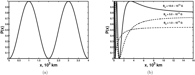
Figure 1: (a) The numerical transition probability versus the distance traveled by a neutrino beam when both resonance conditions, Eqs. (IV) and (22), are satisfied. The parameters of the neutrino system are the following: $\mu=3\times 10^{-12}\thinspace\mu_{\mathrm{B}}$, $\mu_{\nu_{e}}=10^{-13}\thinspace\mu_{\mathrm{B}}$, $\mu_{\nu_{s}}=0$, $E=100\thinspace\mathrm{MeV}$, $m_{\nu_{e}}=1\thinspace\mathrm{eV}$ and $\delta m^{2}=5\times 10^{-17}\thinspace\mathrm{eV}^{2}$. Neutrinos move in background matter with $\rho=10^{6}\thinspace\mathrm{g/cm}^{3}$ and interact with the magnetic field $B=10^{7}\thinspace\mathrm{G}$. (b) The numerical transition probability as a function of the distance in the case of the coordinate dependent magnetic field $B_{\mathrm{dip}}(r)$ for various values of $B_{0}$. The distance $x$ is measured from the inner radius of an envelope $R_{\mathrm{env}}=10^{8}\thinspace\text{cm}$. The parameters of the neutrino system are the same as in the panel (a).

we present the numerical solution of the Schrödinger equation with the Hamiltonians (16) and (20) taking into account the diagonal magnetic moment of an electron neutrino which was neglected while obtaining the resonance conditions since we assumed that $\mu_{a}\ll\mu$. It is necessary to remind that in Ref. Not88 it was found that to get a significant $\nu_{e}^{\mathrm{+{}}}$ luminosity $\sim 10^{50}\thinspace\mathrm{erg/s}$ the diagonal magnetic moment should be $\mu_{\nu_{e}}=10^{-13}\thinspace\mu_{\mathrm{B}}$. We suppose that both Eqs. (IV) and (22) are satisfied. One can see in Fig. 1(a) that diagonal magnetic moments do not significantly influence the dynamics of spin-flavor oscillations since the numerical transition probability practically coincide with the approximate analytical expression $P(x)=\sin^{2}(\mu Bx)$ obtained from Eqs. (16), (20), (IV), and (22) in the limit of small $\mu_{\nu_{e}}$.

We plot Fig. 1(a) in the approximation of constant external fields. Despite the matter density decreases as $1/r^{3}$ inside the envelope Kac02 , we can suppose that it is approximately constant in the shock wave region. However the approximation of the constant magnetic field is quite rough. In Fig. 1(b) we present the solution of the exact Schrödinger equation for the coordinate dependent magnetic field $B_{\mathrm{dip}}(r)$, for various values of the magnetic fields $B_{0}$ at the neutrinosphere. We again suppose that the resonance condition (IV) is fulfilled.

Note that in Sec. II we assumed that the magnetic field is coordinate independent. However, if we suggest that the length of the spatial variation of a magnetic field is much bigger than the typical size of a neutrino wave packet (see also Sec. V), we can neglect it in the analysis of the neutrino wave equation (II). Thus, if this condition is satisfied, the magnetic field is supposed to be spatially constant in deriving main Eqs. (12), (16), and (20) in Secs. II and III. Nevertheless we take into account the magnetic field variation while solving the effective Schrödinger equation with the Hamiltonians (16) and (20). This requirement for spatial variations of magnetic fields can be characterized as the microscopic adiabaticity condition in contrast to the macroscopic adiabaticity typically used in the analysis of neutrino oscillations (see, e.g., Ref. MohPal04 ).

One can see in Fig. 1(b) that at relatively weak magnetic fields $B_{0}\sim 10^{13}\thinspace\text{G}$ the transition probability is a strictly increasing function reaching the asymptotic value $\sim 0.5$ and never is equal to one. This magnetic field corresponds to $B(r=R_{\textrm{env}})=10^{7}\thinspace\text{G}$, where $R_{\textrm{env}}=10^{8}\thinspace\text{cm}$ is the internal radius of an expanding envelope. We should remind that oscillations in a constant magnetic field of such a strength are at resonance, cf. Eq. (22), and hence the transition probability can reach a unit value.

We also notice that at the big distances traveled by neutrinos the transition probability becomes constant. Indeed, using Eqs. (16) and (20) we get that in the limit of the small diagonal magnetic moment of an electron neutrino and if the resonance condition (IV) is fulfilled, at big distances the transition probability has the form, $P(x\gg R_{\textrm{env}})=\sin^{2}(\mu B_{0}R^{3}/2R_{\textrm{env}}^{2})$. The values of the asymptotic transition probability shown in Fig. 1 are in agreement with this expression. At strong magnetic fields ($B_{0}=10^{14}\thinspace\text{G}$ or $B(r=R_{\textrm{env}})=10^{8}\thinspace\text{G}$) the transition probability can reach big values at the outer edge of a broad envelope, $r\sim 10^{9}\thinspace\text{cm}$. Note that analogous behaviour of transition probability was found in Ref. TotSat96 while studying spin-flavor oscillations of Majorana neutrinos in a supernova.

V Analysis of approximations

First we should remind that we use the relativistic quantum mechanics approach, with the external fields being independent of spatial coordinates. If external fields depend on the spatial coordinates, Dirac wave packets theory reveals various additional phenomena such as particles creation by the external field inhomogeneity ItzZub80p60 . For the approximation of the spatially constant external fields to be valid, the typical length scale of the external field variation $L_{\mathrm{ext}}$ should be much greater than the Compton length of a neutrino ItzZub80p60 : $L_{\mathrm{ext}}\gg\lambdabar_{C}=\hbar/m_{\nu}c$ DvoStu02 . For a neutrino with $m_{\nu}\sim 1\thinspace\mathrm{eV}$ this condition reads $L_{\mathrm{ext}}\gg 10^{-5}\thinspace\mathrm{cm}$, that is fulfilled for almost all realistic external fields.

We should also make a remark on the accounting for the mixing potential $V$ in Eq. (10). Eq. (II) contains the nondiagonal term $\sim V$. The analysis of analogous equations is typically made in frames of the perturbation theory LanLif02 using the expansion on powers of the mixing potential, i.e. on the coupling constants which are proportional to $g$ and $\mu B$. As it was mentioned in Sec. II, the wave equations for massive neutrinos in vacuum decouple and the evolution of these states depends on the initial condition only. While solving Eq. (10) we could have taken into account the terms linear in $g$ and $\mu B$ as it was made in Refs. Dvo06 ; DvoMaa07 . However in subsequent calculations, which lead to Eqs. (11) and (12), these coefficients were accounted for exactly.

Now let us discuss other factors which can also give the contributions, comparable with Eq. (20), to the effective Hamiltonian. While deriving the effective Hamiltonian (12) in Sec. II we supposed that the magnetic field is transverse with respect to the neutrino motion. The effect of the longitudinal magnetic field $B_{\parallel{}}$ on neutrino oscillations was studied in Ref. AkhKhl88 . In order to neglect the longitudinal magnetic field contribution in comparison with our correction (20), its strength should satisfy the condition,

$$\frac{B_{\parallel{}}}{B_{\perp{}}}\ll\frac{1}{16kB_{\perp{}}|\mu_{a}m_{a}-\mu_{b}m_{b}|}\left|\frac{m_{a}^{2}g_{a}^{3}}{\mathcal{M}_{a}^{2}}-\frac{m_{b}^{2}g_{b}^{3}}{\mathcal{M}_{b}^{2}}\right|,$$ (23)

where $B_{\perp{}}$ is the transverse component of the magnetic field. The condition (23) is satisfied for neutrinos emitted inside the solid angle near the equatorial plane with the spread $2\vartheta\sim 2B_{\parallel{}}/B_{\perp{}}$. Assuming the radially symmetric neutrino emission we find that about 2% of the total neutrino flux is affected by the new resonance (IV), i.e. the influence of the longitudinal magnetic field is negligible for oscillations of such particles.

The next important approximation made in the deviation of Eq. (12) was the assumption of negligible polarization of matter which can be not true if we study rather strong magnetic fields. The effect of matter polarization on neutrino oscillations was previously discussed in Refs. DvoStu02 ; Nun97 ; LobStu01 . It was found that in the leading order in $m_{a}/k$ matter polarization produces the following contribution to the diagonal entry of the effective Hamiltonian, corresponding to right-handed neutrinos: $g_{a}(\bm{\lambda}_{f}\bm{\beta}_{\nu})(m_{a}/k)$, where $\bm{\beta}_{\nu}$ is the neutrino velocity and $\bm{\lambda}_{f}$ is the mean polarization vector of background fermions. Note that in polarized matter the effective energy of left-handed neutrinos also changes. However this process does not contribute to the considered oscillations channel $\nu_{e}^{\mathrm{+{}}}\leftrightarrow\nu_{s}^{\mathrm{-{}}}$.

It is clear that one should take into account only the polarization of electrons since nucleons are much heavier. Using the results of Refs. Nun97 ; Sum05 we obtain that in the shock wave region electrons are relativistic and weakly degenerate. Finally we get that the new correction to the effective Hamiltonian (20) becomes bigger than the contribution of matter polarization to the effective potential of right-handed neutrinos if the electron temperature exceeds $10\thinspace\mathrm{MeV}$ which is comparable with the mean temperature in an expanding envelope Sum05 .

The presence of relatively big Dirac neutrino magnetic moments implies the existence of new interactions, beyond the standard model, which electromagnetically couple left- and right-handed neutrinos. It is possible that these new interactions also contribute to the effective potential of the right-handed neutrino interaction with background matter. Despite this additional effective potential is likely to be small, one should evaluate it and compare with the correction (20).

The most generic $\mathrm{SU}(2)_{L}\times\mathrm{U}(1)_{Y}$ gauge invariant and remormalizable interaction which produces Dirac neutrino magnetic moment was discussed in Ref. Bel05 . The effective Lagrangian of this interaction involves the dimension $n=6$ operators $\mathcal{O}_{j}$, $\mathcal{L}_{\mathrm{eff}}=(1/\Lambda^{2})\sum_{j}C_{j}\mathcal{O}_{j}+\mathrm{h.c.}$, where $\Lambda\sim 1\thinspace\mathrm{TeV}$ is scale of the new physics, $C_{j}$ are the effective operator coupling constants and sum spans all the operators of the given dimension.

One of the operators $\mathcal{O}_{j}$ also contributes to the effective potential of a right-handed neutrino in matter, $\mathcal{O}=\kappa\bar{L}\tau_{a}\tilde{\phi}\sigma^{\mu\nu}\nu_{\mathrm{R}}W_{\mu\nu}^{a}$, where $\kappa$ is the coupling constant, $\tau_{a}$ are Pauli matrices, $L^{\mathrm{T}}=(\nu_{\mathrm{L}},e_{\mathrm{L}})$ is the $\mathrm{SU}(2)_{L}$ isodoublet, $\tilde{\phi}=\mathrm{i}\tau_{2}\phi^{*{}}$, with $\phi$ being a Higgs field, and $W_{\mu\nu}^{a}=\partial_{\mu}W_{\nu}^{a}-\partial_{\nu}W_{\mu}^{a}-\kappa\epsilon_{abc}W_{\mu}^{b}W_{\nu}^{c}$ is the $\mathrm{SU}(2)_{L}$ field strength tensor. Assuming the spontaneous symmetry breaking at the electroweak scale, $\phi^{\mathrm{T}}\to(0,v/\sqrt{2})$, we can rewrite the contribution of the operator $\mathcal{O}$ to the effective Lagrangian in the form,

$$\mathcal{L}_{\mathrm{eff}}=\frac{C\kappa v}{\sqrt{2}}\bar{e}_{L}\sigma^{\mu\nu}\nu_{R}(W_{\mu\nu}^{1}-{i}W_{\mu\nu}^{2})+\mathrm{h.c.},$$ (24)

which implies that a process $e^{-{}}+\nu_{\mathrm{+{}}}\to e^{-{}}+\nu_{\mathrm{-{}}}$ should happen in background matter.

Using the results of Ref. Bel05 we can evaluate the contribution of the new interactions to the effective Hamiltonian (16) as

$$\delta V_{R}\sim V_{\mathrm{sm}}\frac{|\kappa|^{2}}{G_{\mathrm{F}}M_{W}^{2}}\left(\frac{\mu_{\nu}}{\mu_{\mathrm{B}}}\right)^{2}\left(\frac{E_{\nu}}{m_{e}}\right)^{2},$$ (25)

where $V_{sm}\sim G_{\mathrm{F}}n_{e}$ is the standard model effective potential, $G_{\mathrm{F}}$ is the Fermi constant, and $M_{W}$ is the $W$ boson mass. Taking $\mu_{\nu}\sim 10^{-12}\mu_{\mathrm{B}}$, $E_{\nu}\sim 100\thinspace\mathrm{MeV}$ and $m_{\nu}\sim 0.2\thinspace\mathrm{eV}$ (see Sec. IV) we can get that the ratio of the correction to the effective potential $\delta V_{R}$ and new correction (20) is $\sim 10^{-2}$. It means that the influence of new interactions, which generate neutrino magnetic moments, are not important for neutrino spin-flavor oscillations.

The constraint on the Dirac neutrino magnetic moment obtained in Ref. Bel05 is $10^{-14}\mu_{\mathrm{B}}$. Nevertheless in Sec. IV we used the magnetic moments in the $(10^{-13}-10^{-12})\mu_{\mathrm{B}}$ range since analogous constrains on the Dirac neutrino magnetic moments were obtained in Refs. Not88 ; Raf90 on the basis of the analysis of astrophysical data.

VI Conclusion

In this paper we have described neutrino spin-flavor oscillations in dense matter and strong magnetic field in the frame of relativistic quantum mechanics. The advantage of this formalism, compared to the commonly used quantum mechanical approach, is that one can exactly take into account the neutrino properties like initial momentum, $\delta m^{2}$, mixing angles and magnetic moments, as well as the matter density and the strength of the magnetic field since we used the exact solutions of the Dirac equation for massive neutrinos in presence of external fields.

In Sec. II it was demonstrated that the initial condition problem for the system of two mixed flavor neutrinos, each of them represented as four-component Dirac spinors, can be reduced to a Schrödinger like equation [see Eq. (12)]. In Sec. III it was shown that the Hamiltonian of this evolution equation formally coincides with the previously proposed LimMar88 effective Hamiltonian (16).

It should be, however, noted that the dynamics of neutrino spin-flavor oscillation in matter and magnetic field in frames of the quantum mechanical description is defined by both the effective Hamiltonian and the correct basis of the neutrinos wave functions. In Sec. III we showed that the choice of the helicity eigenstates basis is justified only in the case of the weak magnetic field limit. This kind of basis was used in the previous treatment of neutrino spin-flavor oscillations LimMar88 . The opposite situation of the strong magnetic field and low density matter was also discussed in Sec. III. In this limit the correct basis consists of the eigenfunctions of the operator $\Pi_{a}$.

Besides the demonstration of the consistency of our results with the standard approach for the description of neutrino spin-flavor oscillations, we found the correction (20) to the commonly used effective Hamiltonian (16) which is usually omitted LimMar88 . It was possible to obtain this correction in the explicit form since we used the energy levels (8) and basis spinors (II) which exactly account for external fields.

In Sec. IV we discussed the realistic situation when the correction (20) is important. We considered $\nu_{e}^{\mathrm{+{}}}\leftrightarrow\nu_{s}^{\mathrm{-{}}}$ oscillations channel, where $\nu_{s}$ is the additional sterile neutrino almost degenerate in mass with other neutrino states. The right-handed electron neutrinos were supposed to be produced during the supernova explosion due to the scattering of left-handed neutrinos with the non-zero diagonal magnetic moment on background fermions Not88 . The flux of these right-handed neutrinos was taken to propagate through the expanding envelope and interact with an external magnetic field due to the presence of the non-zero transition magnetic moment.

We found that the new resonance in neutrino spin-flavor oscillations can appear if the strength of the magnetic field and the matter density are close to the values recently discussed in Refs. Aki03 ; Tom05 . Note that new resonance condition (IV) depends on the absolute value of the neutrino mass. Thus the observation of this new resonance would provide the information about the absolute scale of the neutrino masses. Although $\nu_{e}^{\mathrm{+{}}}\leftrightarrow\nu_{s}^{\mathrm{-{}}}$ oscillations do not change the dynamics of a supernova explosion the appearance of this additional resonance channel of neutrino spin-flavor oscillations makes impossible a terrestrial observation of the right-handed supernova neutrinos proposed in Ref. Not88 .

To analyze the dynamics of the Schrödinger equation with exact Hamiltonians (16) and (20) in Sec. IV we presented the numerical transition probability which accounts for all magnetic moments and is built for various magnetic fields configurations. In particular we analyze the constant magnetic field and more realistic coordinate dependent magnetic field of a magnetic dipole $B_{\mathrm{dip}}(r)$. It was revealed that diagonal magnetic moment of an electron neutrino does not significantly influence the transition probability. Then we found that at rather strong magnetic field strength the transition probability can reach big values when a neutrino leaves an expanding envelope.

In Sec. V we considered other factors which can be comparable with the correction obtained (20). We analyzed the contributions of the longitudinal magnetic field and matter polarization which were omitted in the derivation of the effective Hamiltonian (12). In particular we have found that a longitudinal magnetic field is not important for neutrinos emitted near the equator of a star. The matter polarization does not influence the dynamics of neutrino oscillations if the temperature of background electrons is higher than a few MeV. We also evaluated the possible contributions of the new interactions, which generate neutrino magnetic moments Bel05 , to the effective potentials of right-handed neutrinos. It was found that these contributions are negligible compared to the correction (20).

- (1) M. B. Voloshin, M. I. Vysorskiĭ, and L. B. Okun’, Sov. Phys. JETP 64, 446 (1986).
- (2) C.-S. Lim and W. J. Marciano, Phys. Rev. D 37, 1368 (1988).
- (3) M. Fukugita and T. Yanagida, Physics of neutrinos and applications to astrophysics (Berlin, Springer, 2003), pp. 391–394.
- (4) F. T. Avignone, III, S. R. Elliott, and J. Engel, Rev. Mod. Phys. 80, 481 (2008), arXiv:0708.1033 [nucl-ex].
- (5) See pp. 461–479 in Ref. FukYan03p391
- (6) A. G. Beda, et al. (GEMMA Collaboration), Phys. Part. Nucl. Lett. 7, 406 (2010), arXiv:0906.1926 [hep-ex].
- (7) C. Arpesella et al. (BOREXINO Collaboration), Phys. Rev. Lett. 101, 091302 (2008), arXiv:0805.3843 [astro-ph].
- (8) S. I. Blinnikov and N. V. Dunina-Barkovskaya, MNRAS 266, 289 (1994); G. G. Raffelt, Phys. Rept. 320, 319 (1999).
- (9) E. Kh. Akhmedov and J. Pulido, Phys. Lett. B 553, 7 (2003); hep-ph/0209192.
- (10) S. Akiyama, et al., Astrophys. J 584, 954 (2003), astro-ph/0208128.
- (11) M. B. Voloshin, Phys. Lett. B 209, 360 (1988).
- (12) A. B. Balantekin, C. Volpe, and J. Welzel, JCAP 0709, 016 (2007), arXiv:0706.3023 [astro-ph].
- (13) D. Nötzold, Phys. Rev. D 38, 1658 (1988); R. Barbieri and R. N. Mohapatra, Phys. Rev. Lett. 61, 27 (1988); A. Ayala, J. C. D’Olivo, and M. Torres, Nucl. Phys. B 564, 204 (2000), hep-ph/9907398; A. V. Kuznetsov and N. V. Mikheev, JCAP 0711, 204 (2000), arXiv:0709.0110 [hep-ph]; A. V. Kuznetsov, N. V. Mikheev, and A. A. Okrugin, Int. J. Mod. Phys. A 24, 5977 (2009), arXiv:0907.2905 [hep-ph]; O. Lychkovskiy and S. Blinnikov, Phys. Atom. Nucl. 73, 614 (2010), arXiv:0905.3658 [hep-ph].
- (14) M. Dvornikov, Phys. Lett. B 610, 262 (2005), hep-ph/0411101; Phys. Atom. Nucl. 72, 116 (2009), hep-ph/0610047; arXiv:1001.2516 [hep-ph]; M. Dvornikov and J. Maalampi, Phys. Rev. D 79, 113015 (2009), arXiv:0809.0963 [hep-ph].
- (15) M. Dvornikov, Eur. Phys. J. C 47, 437 (2006), hep-ph/0601156.
- (16) M. Dvornikov and J. Maalampi, Phys. Lett. B 657, 217 (2007), hep-ph/0701209.
- (17) M. Dvornikov, J. Phys. Conf. Ser. 110, 082005 (2008), arXiv:0708.2975 [hep-ph].
- (18) M. Dvornikov, J. Phys. G 35, 025003 (2008), arXiv:0708.2328 [hep-ph].
- (19) D. Nötzold and G. G. Raffelt, Nucl. Phys. B 307, 924 (1988); E. Elizalde, E. J. Ferrer, and V. de la Incera, Phys. Rev. D 70, 043012 (2004), hep-ph/0404234; C. M. Ho, D. Boyanovsky, and H. J. de Vega, Phys. Rev. D 72, 085016 (2005), hep-ph/0508294.
- (20) M. Dvornikov and A. Studenikin, JHEP 0209, 016 (2002), hep-ph/0202113.
- (21) A. E. Bernardini and S. De Leo, Phys. Rev. D 70, 053010 (2004), hep-ph/0411134; Eur. Phys. J. C 37, 471 (2004), hep-ph/0411153; Phys. Rev. D 71, 076008 (2005), hep-ph/0504239.
- (22) K. Zuber, Neutrino physics (Bristol, IOP Publishing, 2004), pp. 19–22.
- (23) A. Studenikin and A. Ternov, Phys. Lett. B 608, 107 (2005), hep-ph/0412408; A. E. Lobanov, Phys. Lett. B 619, 136 (2005), hep-ph/0506007.
- (24) C. Giunti and A. Studenikin, Phys. Atom. Nucl. 72, 2089 (2009), arXiv:0812.3646 [hep-ph].
- (25) C. Itzykson and J.-B. Zuber, Quantum field theory (NY, McGraw-Hill, 1980), p. 693.
- (26) P. Keränen, et al., Phys. Lett. B 574, 162 (2003), hep-ph/0307041; ibid. 597, 374 (2004), hep-ph/0401082; J. Maalampi and J. Riittinen, Phys. Rev. D 81, 037301 (2010), arXiv:0912.4628 [hep-ph]; A. Esmaili, Phys. Rev. D 81, 013006 (2010), arXiv:0909.5410 [hep-ph]; V. A. Kutvitskiĭ, V. B. Semikoz, and D. D. Sokoloff, Astron. Rep. 53, 166 (2009), arXiv:0809.3172 [astro-ph]; C. R. Das, J. Pulido, and M. Picariello, Phys. Rev. D 79, 073010 (2010), arXiv:0902.1310 [hep-ph].
- (27) C. Giunti and C. W. Kim, Fundamentals of neutrino physics and astrophysics (Oxford, Oxford Univ. Press, 2007), pp. 229–231.
- (28) E. Kh. Akhmedov, A. Lanza, and D. W. Sciama, Phys. Rev. D 56, 6117 (1997), hep-ph/9702436.
- (29) R. Tòmas, et al., JCAP 0409, 015 (2004), astro-ph/0407132.
- (30) A. M. Malinovsky, et al., Astron. Lett. 34, 445 (2008).
- (31) G. G. Raffelt, Phys. Rev. Lett. 90, 2856 (1990).
- (32) M. Kachelrieß, et al., Phys. Rev. D 65, 073016 (2002), hep-ph/0108100.
- (33) R. N. Mohapatra and P. B. Pal, Massive neutrinos in physics and astrophysics (Singapore, World Scientific, 2003), 3rd ed., pp. 101–106.
- (34) T. Totani and K. Sato, Phys. Rev. D 54, 5975 (1996), astro-ph/9609035.
- (35) See pp. 60–63 in Ref. ItzZub80 .
- (36) L. D. Landau and E. M. Lifschitz, Quantum mechanics: Nonrelativistic theory (Oxford, Pergamon, 1991), pp. 142–146.
- (37) E. Kh. Akhmedov and M. Yu. Khlopov, Sov. J. Nucl. Phys. 47, 689 (1988).
- (38) H. Nunokawa, et al., Nucl. Phys. B 501, 17 (1997), hep-ph/9701420.
- (39) A. E. Lobanov, and A. I. Studenikin, Phys. Lett. B 515, 94 (2001), hep-ph/0106101. A. Grigiriev, A. Lobanov, and A. Studenikin, Phys. Lett. B 535, 187 (2002), hep-ph/0202276.
- (40) K. Sumiyoshi, et al., Astrophys. J. 629, 922 (2005), astro-ph/0506620.
- (41) N. F. Bell, et al., Phys. Rev. Lett. 95, 151802 (2005), hep-ph/0504134.