Weak gravitational lensing with Deimos

Abstract

We introduce a novel method for weak-lensing measurements, which is based on a mathematically exact deconvolution of the moments of the apparent brightness distribution of galaxies from the telescope’s PSF. No assumptions on the shape of the galaxy or the PSF are made. The (de)convolution equations are exact for unweighted moments only, while in practice a compact weight function needs to be applied to the noisy images to ensure that the moment measurement yields significant results. We employ a Gaussian weight function, whose centroid and ellipticity are iteratively adjusted to match the corresponding quantities of the source. The change of the moments caused by the application of the weight function can then be corrected by considering higher-order weighted moments of the same source. Because of the form of the deconvolution equations, even an incomplete weighting correction leads to an excellent shear estimation if galaxies and PSF are measured with a weight function of identical size.

We demonstrate the accuracy and capabilities of this new method in the context of weak gravitational lensing measurements with a set of specialized tests and show its competitive performance on the GREAT08 challenge data. A complete C++ implementation of the method can be requested from the authors.

1 Introduction

Shear estimation from noisy galaxy images is a challenging task, even more so for the stringent accuracy requirements of upcoming cosmic shear surveys. Existing methods can achieve multiplicative errors in the percent range (Bridle et al., 2010), but to exploit the statistical power of the next-generation surveys errors in the permille range or even below are requested (Amara & Réfrégier, 2008).

Shear estimates can be achieved in a model-based or in a model-independent fashion. For instance, Lensfit (Miller et al., 2007) compares sheared and convolved bulge-disk profiles to the given galaxies. Model-based approaches often perform excellently for strongly degraded data because certain implicit or explicit priors keep the results within reasonable bounds, e.g. the source ellipticity smaller than unity. On the other hand, when imposing these priors to data, whose characteristics differ from the expectation, these approaches may also bias the outcome.

Model-independent approaches do not – or at least not as strongly – assume particular knowledge of the data to be analyzed. They should therefore generalize better in applications, where priors are not obvious, e.g. on the intrinsic shape of lensed galaxies. The traditional KSB method (Kaiser et al., 1995) forms a shear estimator from the second-order moments of lensed galaxy images. When doing so, it is not guaranteed that reasonable shear estimates can be achieved for each galaxy. Consequently, KSB requires a careful setup, which is adjusted to the characteristics of the data to be analyzed. KSB furthermore employs strong assumptions on the PSF shape, which are not necessarily fulfilled for a given telescope or observation (Kuijken, 1999). As we have shown recently, KSB relies on several other assumptions concerning the relation between convolved and unconvolved ellipticity as well as the relation between ellipticity and shear, neither of which hold in practice (Viola et al., 2011).

In this work we present a novel method for shear estimation, which maintains the strengths of model-independent approaches by working with multipole moments, but does not suffer from the KSB-shortcomings mentioned above.

2 The DEIMOS method

The effect of gravitational lensing on the surface brightness distribution $G(\mathbf{x})$ of a distant background galaxies is most naturally described in terms of the moments of the brightness distribution,

$$\{G\}_{i,j}\equiv\int d^{2}x\ G(\mathbf{x})\,x_{1}^{i}x_{2}^{j},$$ (1)

for which we introduce a tensor-like notation. The effect of the reduced shear $\mathbf{g}$ is contained in the change of the complex ellipticity

$$\mn@boldsymbol{\chi}\equiv\frac{\{G\}_{2,0}-\{G\}_{0,2}+2\mathrm{i}\{G\}_{1,1}}{\{G\}_{2,0}+\{G\}_{0,2}}$$ (2)

with respect to its value before lensing,

$$\mn@boldsymbol{\chi}^{s}=\frac{\mn@boldsymbol{\chi}-2\mathbf{g}+\mathbf{g}^{2}\mn@boldsymbol{\chi}^{\star}}{1+|\mathbf{g}|^{2}-2\Re(\mathbf{g}\mn@boldsymbol{\chi}^{\star})}$$ (3)

(e.g. Bartelmann & Schneider, 2001). Unfortunately, we do not know $\mn@boldsymbol{\chi}^{s}$, which would allow solving directly for $\mathbf{g}$ given $\mn@boldsymbol{\chi}$. Furthermore, (at least) two observational complications alter the source’s moments, typically much more drastically than lensing: convolution with the PSF and any means of noise reduction – normally weighting with a compact function – to yield significant moment measurements. Hence, $\mn@boldsymbol{\chi}$ is not directly accessible and needs to be estimated by properly accounting for the observation effects. We leave the treatment of weighting for section 3 and start with the derivation of the change of the moments under convolution.

Any square-integrable one-dimensional function $G(x)$, has an exact representation in Fourier space,

$$G(x)\rightarrow\phi_{G}(k)=\int dx\,G(x)\,\mathrm{e}^{\mathrm{i}kx}.$$ (4)

In the field of statistics, $\phi_{G}$ is often called the characteristic function of $G$ and has a notable alternative form

$$\phi_{G}(k)=\sum_{n}^{\infty}\{G\}_{n}\frac{(\mathrm{i}k)^{n}}{n!},$$ (5)

which provides a link between the Fourier-transform of $G$ and its moments $\{G\}_{n}$, the one-dimensional pendants to Equation 1. We can now employ the convolution theorem, which allows us to replace the convolution by a product in Fourier-space, i.e. by a product of characteristic functions of $G$ and of the PSF kernel $P$,

$$G^{\star}(x)\equiv\int dx^{\prime}\,G(x)\,P(x-x^{\prime})\rightarrow\phi_{G^{\star}}=\phi_{G}\,\phi_{P}.$$ (6)

For convenience, we assume throughout this work the PSF to be flux-normalized, $\{P\}_{0}=1$. Considering Equation 5, we get

$$\begin{split}\phi_{G^{\star}}(k)&=\Bigl{[}\sum_{n}^{\infty}\{G\}_{n}\frac{(\mathrm{i}k)^{n}}{n!}\Bigr{]}\Bigl{[}\sum_{n}^{\infty}\{P\}_{n}\frac{(\mathrm{i}k)^{n}}{n!}\Bigr{]}\\ &=\sum_{n}^{\infty}\sum_{m}^{n}\{G\}_{m}\frac{(\mathrm{i}k)^{m}}{m!}\{P\}_{n-m}\frac{(\mathrm{i}k)^{n-m}}{(n-m)!}\\ &=\sum_{n}^{\infty}\Bigl{[}\sum_{m}^{n}\tbinom{n}{m}\{G\}_{m}\{P\}_{n-m}\Bigr{]}\frac{(\mathrm{i}k)^{n}}{n!},\end{split}$$ (7)

where we applied the Cauchy product in the second step. The expression in square brackets on the last line is by definition the desired moment,

$$\{G^{\star}\}_{n}=\sum_{m}^{n}\tbinom{n}{m}\{G\}_{m}\{P\}_{n-m}.$$ (8)

Hence, we can now express a convolution of the function $G$ with the kernel $P$ entirely in moment space. Moreover, even though the series in Equation 5 is infinite, the order of the moments occurring in the computation of $\{G^{\star}\}_{n}$ is bound by $n$. This means, for calculating all moments of $G^{\star}$ up to order $n$, the knowledge of the same set of moments of $P$ and $G$ is completely sufficient. This results hold for any shape of $G$ and $P$ as long as their moments do not diverge. For non-pathological distributions, this requirement does not pose a significant limitation.

An identical derivation can be performed for two-dimensional moments, which yields the change of moments of $G(\mathbf{x})$ under convolution with the kernel $P(\mathbf{x})$ (Flusser & Suk, 1998):

$$\{G^{\star}\}_{i,j}=\sum_{k}^{i}\sum_{l}^{j}\tbinom{i}{k}\tbinom{j}{l}\{G\}_{k,l}\{P\}_{i-k,j-l}\,.$$ (9)

Deconvolution

To obtain the deconvolved moments required for the shear estimation via the ellipticity $\mn@boldsymbol{\chi}$, we need to measure the moments up to second order of the convolved galaxy shape and of the PSF kernel shape. Then we can make use of a remarkable feature of Equation 9, which is already apparent from its form: The impact of convolution on a moment of order $i+j=n$ is only a function of unconvolved moments of lower order and PSF moments of at most the same order. We can therefore start in zeroth order, the flux, which only needs to be corrected if the PSF is not flux-normalized. With the accurate value of the zeroth order and the first moments of the PSF, we can correct the first-order moments of the galaxy, and so on (cf.Table 1). The hierarchical build-up of the deconvolved moments is the heart of the Deimos method (short for deconvolution in moment space).

It is important to note and will turn out to be crucial for weak-lensing applications that with this deconvolution scheme we do not need to explicitly address the pixel noise, which hampers most other deconvolution approaches in the frequency domain, simply because we restrict ourselves to inferring the most robust low-order moments only.

Table 1: Equations for deconvolving all moments up to order $n=2$. The shown equations are specializations of Equation 9.

$\{G\}_{0,0}\ \{P\}_{0,0}=\{G^{\star}\}_{0,0}$

$\{G\}_{0,1}\ \{P\}_{0,0}=\{G^{\star}\}_{0,1}-\{G\}_{0,0}\ \{P\}_{0,1}$

$\{G\}_{1,0}\ \{P\}_{0,0}=\{G^{\star}\}_{1,0}-\{G\}_{0,0}\ \{P\}_{1,0}$

$\{G\}_{0,2}\ \{P\}_{0,0}=\{G^{\star}\}_{0,2}-\{G\}_{0,0}\ \{P\}_{0,2}-2\{G\}_{0,1}\ \{P\}_{0,1}$

$\{G\}_{1,1}\ \{P\}_{0,0}=\{G^{\star}\}_{1,1}-\{G\}_{0,0}\ \{P\}_{1,1}-\{G\}_{0,1}\ \{P\}_{1,0}-\{G\}_{1,0}\ \{P\}_{0,1}$

$\{G\}_{2,0}\ \{P\}_{0,0}=\{G^{\star}\}_{2,0}-\{G\}_{0,0}\ \{P\}_{2,0}-2\{G\}_{1,0}\ \{P\}_{1,0}$

3 Noise and weighting

In practice, the moments are measured from noisy image data,

$$I(\mathbf{x})=G(\mathbf{x})+N(\mathbf{x}),$$ (10)

where the noise $N$ can be considered to be independently drawn from a Gaussian distribution with variance $\sigma_{n}^{2}$, i.e. $\langle N(\mathbf{x}_{i})N(\mathbf{x}_{j})\rangle=\sigma_{n}^{2}\delta_{ij}$ for any two positions $\mathbf{x}_{i}$ and $\mathbf{x}_{j}$. According to Equation 1, the image values at large distances from the galactic center have the largest impact on the $\langle I\rangle_{n}$ if $n>0$. For finite and compact brightness distributions $G$, these values are dominated by the noise process instead of the galaxy, whose moments we seek to measure. Consequently, centered weight functions $W$ of finite width are typically introduced to limit the integration range in Equation 1 to regions in which $I$ is mostly determined by $G$,

$$I_{w}(\mathbf{x})\equiv W(\mathbf{x})\,I(\mathbf{x}).$$ (11)

A typical choice for $W$ is a circular Gaussian centered at the galactic centroid,

$$W(\mathbf{x})\equiv\exp\Bigl{(}-\frac{\mathbf{x}^{2}}{2s^{2}}\Bigr{)}.$$ (12)

Alternatively, one can choose to optimize the weight function to the shape of the source to be measured. Bernstein & Jarvis (2002, see their section 3.1.2) proposed the usage of a Gaussian, whose centroid $\mathbf{x}_{c}$, size $s$, and ellipticity $\mn@boldsymbol{\epsilon}$ are matched to the source, such that the argument of the exponential in Equation 12 is modified according to

$$\mathbf{x}\to\mathbf{x}^{\prime}=\begin{pmatrix}1-\epsilon_{1}&-\epsilon_{2}\\ -\epsilon_{2}&1+\epsilon_{1}\end{pmatrix}(\mathbf{x}-\mathbf{x}_{c}).$$ (13)

As such a weight function represents a matched spatial filter, it optimizes the significance and accuracy of the measurement if its parameters are close to their true values. This can, however, not be guaranteed in presence of pixel noise, but we found the iterative algorithm proposed by Bernstein & Jarvis (2002) to converge well in practice and therefore employ it to set the weight function within the Deimos method.

Unfortunately, a product in real space like the one in Equation 11 translates into a convolution in Fourier-space. We therefore have to expect some amount of mixing of the moments of $I_{w}$. Even worse, an attempt to relate the moments of $I_{w}$ to those of $I$ leads to diverging integrals. Hence, there is no exact way of incorporating spatial weighting to the moment approach outlined above. On the other hand, we can invert Equation 11 for $I=I_{w}/W$ and expand $1/W$ in a Taylor series around the center at $\mathbf{x}=\mathbf{0}$,

$$\begin{split}W^{-1}(\mathbf{x})\ \approx\ &W^{-1}(\mathbf{0})-W^{\prime}(\mathbf{0})\Bigl{[}\sum_{k=1}^{2}c_{k}x_{k}^{2}\ +4\epsilon_{2}x_{1}x_{2}\Bigr{]}\ +\\ &\frac{1}{2}W^{\prime\prime}(\mathbf{0})\Bigl{[}\sum_{k,l=1}^{2}c_{k}c_{l}x_{k}^{2}x_{l}^{2}-8\epsilon_{2}\sum_{k=1}c_{k}x_{k}^{2}x_{1}x_{2}+(4\epsilon_{2}x_{1}x_{2})^{2}\Bigr{]},\end{split}$$ (14)

where we employed $W^{\prime}(\mathbf{x})\equiv\frac{dW(\mathbf{x})}{d\mathbf{x}^{2}}$ and $c_{1,2}\equiv(1\mp\epsilon_{1})^{2}+\epsilon_{2}^{2}$. We introduce the parameter $n_{w}$ as the maximum order of the Taylor expansion, here $n_{w}=4$. Inserting this expansion in Equation 1, we are able to approximate the moments of $I$ by their deweighted counterparts $\{I_{dw}\}$. For convenience we give the correction terms for orders $n_{w}\leq 6$ in Table 2. This linear expansion allows us to correct for the weighting-induced change in the moments of a certain order $n$ by considering the impact of the weight function on weighted moments up to order $n+n_{w}$.

Table 2: Correction terms for deweighting moments of order $n=i+j$. The deweighted moments $\{I_{dw}\}_{i,j}$ are given by the sum of the correction terms up to the limiting order $n_{w}$.

$n_{w}$	correction terms
0	$\{I_{w}\}_{i,j}$
2	$\frac{1}{2s^{2}}\Bigl{[}c_{1}\{I_{w}\}_{i+2,j}-4\,\epsilon_{2}\{I_{w}\}_{i+1,j+1}+c_{2}\{I_{w}\}_{i.j+2}\Bigr{]}$
4	$\frac{1}{8s^{4}}\Bigl{[}c_{1}^{2}\{I_{w}\}_{i+4,j}-8\,c_{1}\epsilon_{2}\{I_{w}\}_{i+3,j+1}+\bigl{[}2\,c_{1}c_{2}+16\,\epsilon_{2}^{2}\bigr{]},\{I_{w}\}_{i+2,j+2}\ -$
	$\phantom{\frac{1}{8s^{4}}\Bigl{[}}8\,c_{2}\epsilon_{2}\{I_{w}\}_{i+1,j+3}+c_{2}^{2}\{I_{w}\}_{i,j+4}\Bigr{]}$
6	$\frac{1}{48s^{6}}\Bigl{[}c_{1}^{3}\{I_{w}\}_{i+6,j}-12\,c_{1}^{2}\epsilon_{2}\{I_{w}\}_{i+5,j+1}+\bigl{[}3\,c_{1}^{2}c_{2}+48\,c_{1}\epsilon_{2}^{2}\bigr{]}\,\{I_{w}\}_{i+4,j+2}\ -$
	$\phantom{\frac{1}{48s^{6}}\Bigl{[}}\bigl{[}24\,c_{1}c_{2}\epsilon_{2}+64\,\epsilon_{2}^{3}\bigr{]}\,\{I_{w}\}_{i+3,j+3}\ +\,\bigl{[}3\,c_{1}c_{2}^{2}+48\,c_{2}\epsilon_{2}^{2}\bigr{]}\,\{I_{w}\}_{i+2,j+4}\ -$
	$\phantom{\frac{1}{48s^{6}}\Bigl{[}}12\,c_{2}^{2}\epsilon_{2}\{I_{w}\}_{i+1,j+5}+c_{2}^{3}\{I_{w}\}_{i,j+6}\Bigr{]}$

3.1 Deweighting bias

The truncation of the Taylor expansion constitutes the first and only source of bias in the Deimos method. The direction of the bias is evident: As the weight function suppresses contributions to the moments from pixel far away from the centroid, its employment reduces the power in any moment by an amount, which depends on the shape – particularly on the radial profile – of the source and the width $s$. Additionally, if the ellipticity $\mn@boldsymbol{\epsilon}$ was misestimated during the matching of $W$, the measured ellipticity of the source $\mn@boldsymbol{\chi}$ before and after deweighting will be biased towards $\mn@boldsymbol{\epsilon}$. In the realistic case of noisy images, which we address in more detail in subsection 3.2, $\mn@boldsymbol{\epsilon}$ can be wrong in two ways: statistically and systematically. The centered Gaussian distribution of the pixel noise leads to a centered Cauchy-type error distribution of both components of $\mn@boldsymbol{\epsilon}$, i.e. the statistical errors of $\mn@boldsymbol{\epsilon}$ and therefore also $\chi$ have vanishing mean. The systematic errors stem from the application of a compact weight function to measure $\epsilon$, which for any finite $s$ constitutes a removal of information. This leads to deviations of the measured $\mn@boldsymbol{\epsilon}$ from the true $\mn@boldsymbol{\epsilon}$ if e.g. the centroid is not determined accurately or the ellipticity changes with radius. For individual objects, these deviations are impossible to quantify precisely – as this would require knowledge of the true observed morphology – and hamper all weak-lensing measurements unless an appropriate treatment is devised (e.g. Hosseini & Bethge, 2009; Bernstein, 2010). For large ensembles of galaxies, effective levels of systematic errors can be assessed by analyzing dedicated simulations (cf. section 4).

We investigate now the Deimos-specific systematic impact of a finite $n_{w}$ on the recovery of the deweighted moments. For the experiments in this section we simulated simple galaxy models following the Sérsic profile

$$p_{s}(r)\propto\exp\Bigl{\{}-b_{n_{s}}\Bigl{[}\Bigl{(}\frac{r}{R_{e}}\Bigr{)}^{1/n_{s}}-1\Bigr{]}\Bigr{\}},$$ (15)

where $n_{s}$ denotes the Sérsic index, and $R_{e}$ the effective radius, while the PSFs are modeled from the Moffat profile

$$p_{m}(r)\propto(1+\alpha r^{2})^{-\beta},$$ (16)

where $\alpha=\bigl{(}2^{1/\beta}-1\bigl{)}/\bigl{(}\mathrm{FWHM}/2\bigr{)}^{2}$ sets the width of the profile and $\beta$ its slope. Both model types acquire their ellipticity according to Equation 13

In the top panel of Figure 1 we show the error after deweighting a convolved galaxy image from a matched elliptical weight function as a function of its size $s$. As noted above, the bias is always negative and is clearly more prominent for the larger disk-type galaxy (circle markers). As the Taylor expansion becomes more accurate for $n_{w}\to\infty$ or $s\to\infty$, the bias of any moment decreases accordingly.

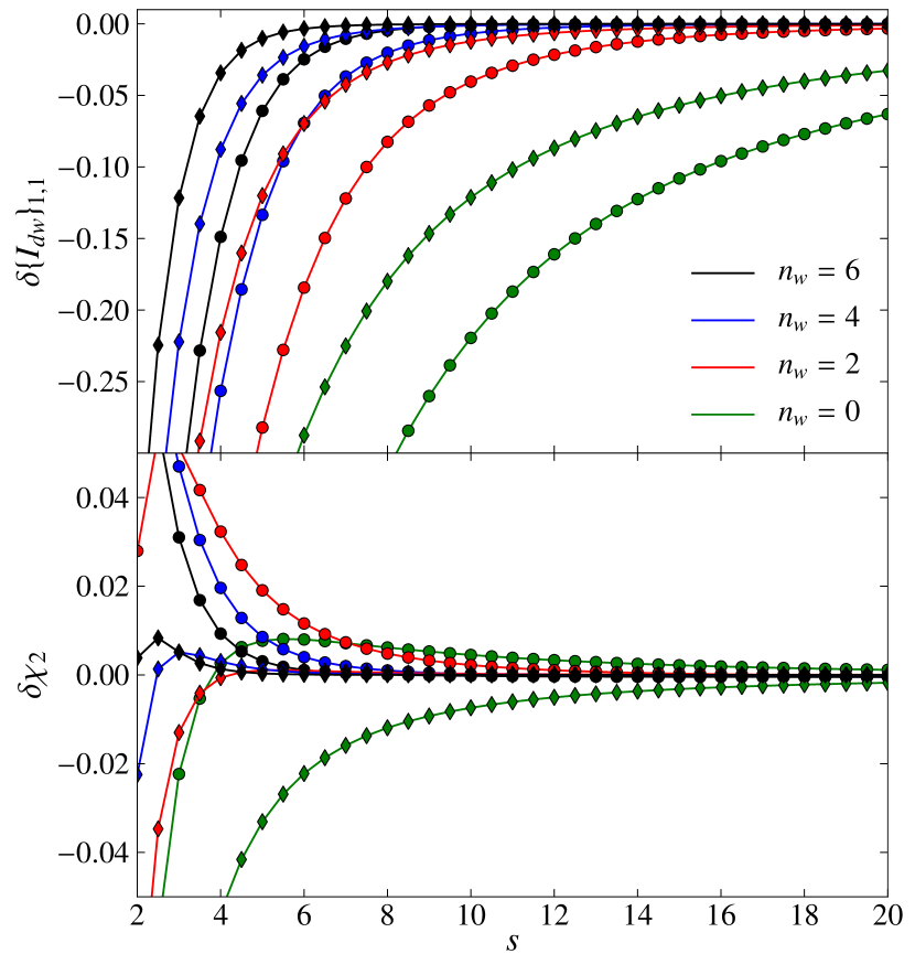
Figure 1: Weighting-induced bias. Relative error of the PSF-convolved and deweighted moment $\{I_{dw}\}_{1,1}$ (top) and of the estimated ellipticity after deconvolution (bottom) as a function of weight function size $s$. Colors indicate the correction order $n_{w}$, while markers denote the galaxy model (circles for model 1, diamonds for model 2). The galaxy models are simulated as Sérsic profiles with the following parameters: $\mn@boldsymbol{\epsilon}^{s}=(0.1,0.4),\ n_{s}=1\,(4),\ R_{e}=3\,(1.5)$ for model 1 (2). The PSF was of Moffat-type with $\mn@boldsymbol{\epsilon}=(0.05,0.05),\ \beta=3,\ \mathrm{FWHM}=3$. The weight functions of galaxy and PSF had the same size $s$, but individually matched ellipticities.

An important consequence of the employment of a weight function with matched ellipticity is that the bias after deweighting does only very weakly depend on the apparent ellipticity, i.e. all moments of the same order are biased by the same relative factor $\Delta(n,s)$. This means any ratio of such moments remains unbiased. This does not guarantee that the ellipticity is still unbiased after the moments have passed the deconvolution step, which is exact only for unweighted moments. On the other hand, the particular form of the equations in Table 1 becomes important here: If we assume well-centered images of the galaxy and the PSF and a negligible error of the source flux $\{G\}_{0,0}$, none of which is guaranteed for faint objects, the deconvolution equations for the relevant second-order moments only mix second-order moments. If furthermore $\Delta_{G}(2,s)=\Delta_{P}(2,s)$, the ellipticity $\mn@boldsymbol{\chi}$ (cf. Equation 2) will remain unbiased after deconvolution even though the moments themselves were biased. The aforementioned condition holds if the radial profiles of PSF and galaxy are similar within the weight function, in other words, if the galaxy is small. This behavior can clearly be seen in the bottom panel of Figure 1, where the ellipticity estimate of the smaller elliptical galaxy (diamond markers) has sub-percent bias for $n_{w}\geq 2$ and $s\geq 3$. The estimates for the larger galaxy are slightly higher because $|\Delta_{G}(2,s)|>|\Delta_{P}(2,s)|$, i.e. the deconvolution procedure overcompensates the PSF-induced change of the moments. However, sub-percent bias is achieved for $n_{w}\geq 4$ and $s\geq 5$.

For large galaxies, it might be advantageous to adjust the sizes of galaxy and PSF independently as this would render $\Delta_{G}(2,s_{G})$ more comparable to $\Delta_{P}(2,s_{P})$. However, we found employing a common size $s$ for both objects to be more stable for the small and noisy galaxy images typically encountered in weak-lensing applications. We therefore adjust the size $s$ such as to allow an optimal measurement of the deweighted PSF moments. Since the main purpose of the weighting is the reduction of noise in the measured moments, one could improve the presented scheme by increasing $s$ for galaxies with larger surface brightness such as to reduce the bias when the data quality permits.

3.2 Deweighting variance

Being unbiased in a noise-free situation does not suffice for a practical weak-lensing application as the image quality is strongly degraded by pixel noise. We therefore investigate now the noise properties of the deweighted and deconvolved moments.

The variance of the weighted moments is given by

$$\sigma^{2}\bigl{(}\{I_{w}\}_{i,j}\bigr{)}=\sigma_{n}^{2}\int d\mathbf{x}\ W^{2}(\mathbf{x})\,x_{1}^{2i}x_{2}^{2j}$$ (17)

since the noise is uncorrelated and has a vanishing mean. It is evident from Table 2 that the variance of the deweighted moments increases with the number of contributing terms, i.e. with $n_{w}$. Less obvious is the response under changes of $s$. While each moment accumulates more noise with a wider weight function, the prefactors of the deweighting correction terms is proportional to $s^{-n_{w}}$ such that their impact is reduced for larger $s$.

To quantitatively understand the impact of $n_{w}$ and $s$ in a fairly realistic scenario we simulated 10,000 images of the galaxy models 1 and 2 from the last section. We drew their intrinsic ellipticities from a Rayleigh distribution with $\sigma_{|\epsilon^{s}|}=0.3$. Their flux was fixed at unity, and the images were degraded by Gaussian pixel noise with variance $\sigma_{n}^{2}$. We ran Deimos on each of these image sets with a fixed scale $s$. The results are presented in Figure 2, where we show the dispersion of the measured $\mn@boldsymbol{\chi}$ in units of the dispersion of $\mn@boldsymbol{\chi}^{s}$. From the left panel it becomes evident that the attempt of measuring unbiased ellipticities (large $n_{w}$ or $s$) comes at the price of increased noise in the estimates. Considering also Figure 1, we infer that in this bias-variance trade-off small values of $s$ and large values of $n_{w}$ should be favored since this provides estimates with high accuracy and a moderate amount of noise.

In the right panel of Figure 2 we show the estimator noise as function of the pixel noise. Equation 17 suggests that there should be a linear relation between these two quantities, which is roughly confirmed by the plot. Additional uncertainties in the moment measurement – caused by e.g. improper centroiding – and the non-linear combinations of second-order moments to form $\mn@boldsymbol{\chi}$ lift the actual estimator uncertainty beyond the linear prediction.

Even though the true errors of $\mn@boldsymbol{\chi}$ may not exactly follow the linear theory, we will now exploit the fairly linear behavior to form error estimates. We can express the deweighting procedure as a matrix mapping,

$$\{\mathbf{I}_{dw}\}=\textbf{{D}}\cdot\{\mathbf{I}_{w}\},$$ (18)

where $\{\mathbf{I}_{w}\}$ and $\{\mathbf{I}_{dw}\}$ denote the vectors of all weighted and deweighted moments, and D encodes the correction terms of Table 2. The diagonal covariance matrix $\textbf{{S}}_{w}$ of the weighted moment variances given by Equation 17 is related to the covariance matrix of the deweighted moments by

$$\textbf{{S}}_{d}=\textbf{{D}}\cdot\textbf{{S}}_{w}\cdot\textbf{{D}}^{T},$$ (19)

from which we can obtain the marginalized errors by

$$\Bigl{(}\sigma^{2}\bigl{(}\{I_{dw}\}_{i,j}\bigr{)}\Bigl{)}^{-1}=\Bigl{(}\textbf{{S}}_{d}^{-1}\Bigr{)}_{k,k},$$ (20)

where $k$ denotes the position of the moment $\{I_{d}\}_{i,j}$ in the vector $\{\mathbf{I}_{dw}\}$. Under the assumptions mentioned above, also the deconvolution can be considered a linear operation, at least up to order 2, so that we can extend the error propagation even beyond this step: If we neglect errors in the PSF moments, the errors of the deconvolved moments (up to order 2) are identical to those of the deweighted ones. We can therefore estimate the errors of all quantities based on deconvolved moments directly from Equation 20.

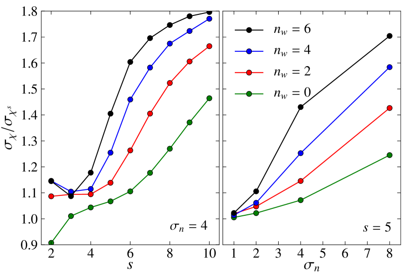
Figure 2: Noise of the deweighted and deconvolved ellipticity estimate as a function of the weight function size $s$ (left) and of the standard deviation of the pixel noise $\sigma_{n}$ (right). The color and marker code is explained in Figure 1. The pixel noise is given in units of $10^{-3}$ for flux-normalized sources. $\sigma_{n}=8$ is close to the detection limit for this source model.

4 Shear accuracy tests

So far, we were concerned with the estimation of ellipticity. To test the ability of our new method to estimate the shear, we make use of the reference simulations with realistic noise levels from the GREAT08 challenge (Bridle et al., 2010). As the shear values in these simulations are fairly low, we employ the linearized version of Equation 3, corrected by the shear responsivity of the source ensemble,

$$\tilde{\mathbf{g}}=\frac{\langle\mn@boldsymbol{\chi}\rangle}{2-\sigma_{\chi}^{2}}$$ (21)

(e.g. Massey et al., 2007), without any further weighting of individual galaxies, to translate Deimos ellipticity measures into shear estimates. The dispersion $\sigma_{\chi}^{2}$ is measured from the lensed and noisy galaxy images and hence only coarsely describes the intrinsic shape dispersion (cf. Figure 2). We are aware of this limitation and verified with additional simulations that it introduces sub-percent biases for the range of shears and pixel noise levels we expect from the GREAT08 images.

We inferred the weight function size $s=4$ and the correction order $n_{w}=4$ from the optimal outcome for a set with known shears. The actual GREAT08 challenge data comprises 9 different image sets, which differ in the shape of the PSF, the signal-to-noise ratio, the size, and the model-type of galaxies. For each of these branches, there are 300 images with different values of shear. We performed the Deimos analysis of all images keeping the weighting parameters fixed to the values inferred before. The results are shown in Figure 3 in terms of the GREAT08 quality metric $Q$ (see eqs. 1& 2 in Bridle et al., 2010) and of the multiplicative shear accuracy parameters $m_{i}$ obtained from a linear fit of the shear estimates $\tilde{g}_{i}$ to the true shear values $g_{i}$ (Heymans et al., 2006; Massey et al., 2007),

$$\tilde{g}_{i}-g_{i}=m_{i}\,g_{i}+c_{i}.$$ (22)

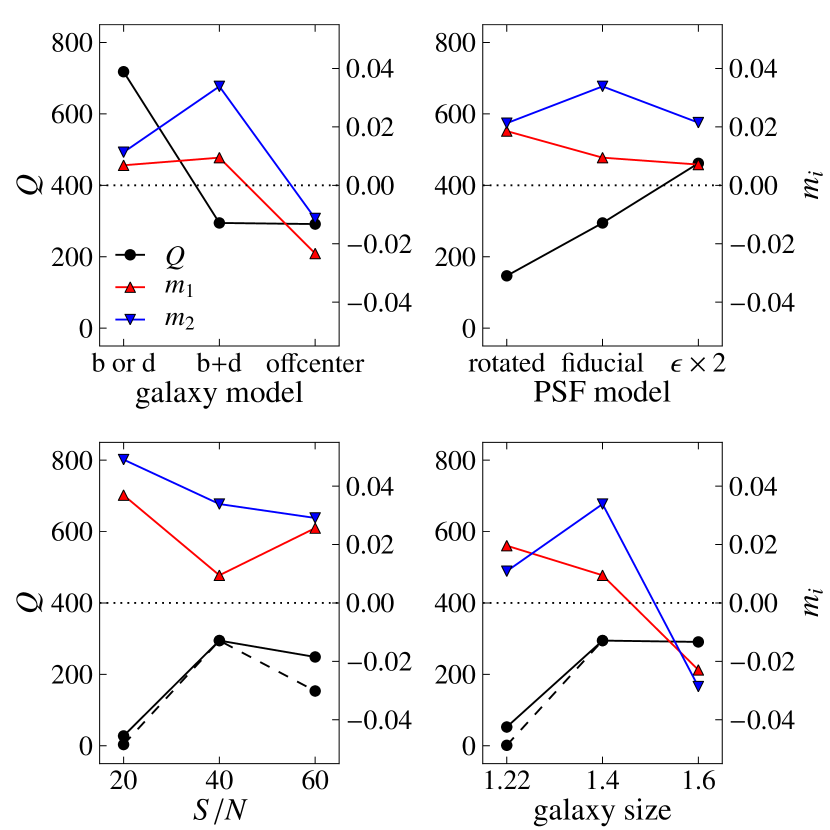
Figure 3: GREAT08 $Q$ metric and multiplicative shear accuracy $m_{i}$ for the nine different branches of the GREAT08 challenge data with realistic noise levels. In each panel, the scale on the left describes the values of $Q$ and the scale on the right the values of $m_{i}$. The dotted line denotes $m_{i}=0$. The dashed lines show the $Q$-value before we adjusted the weight-function matching and deweighting parameters to the source characteristics of the branch.

From Figure 3 we clearly see the highly competitive performance of Deimos with a typical $Q>200$ in all but two branches. Single-component galaxy models yield a particularly large $Q$-value, probably because the bulge-only models are the most compact ones and thus favor the setting of a constant $s$ for PSF and galaxies. In terms of $Q$, there is no change between the centered and the off-centered double-component galaxy models, but both $m_{i}$ drop for the off-centered ones. As such galaxy shapes have variable ellipticity with radius and Deimos measures them with a fixed weight function size, we interpret this as a small but noticeable ellipticity-gradient bias (Bernstein, 2010).

The response to changes in the PSF shape is a bit more worrisome and requires explanation. The fiducial PSF had $\epsilon_{1}>\epsilon_{2}$, and the opposite is true for the rotated one. From all panels of Figure 3 we can see that typically $|m_{1}|<|m_{2}|$. Such a behavior has already been noted by Massey et al. (2007): Because a square pixel appears larger in diagonal direction than along the pixel edges, the moment $\{I\}_{11}$ and hence $\epsilon_{2}$ suffer more strongly from the finite size of pixels. From the discussion in subsection 3.1, we expect a certain amount of PSF-overcompensation for small weighting function sizes. As the PSF shape is most strongly affected by pixelation, the overcompensation boosts preferentially those galaxy moments, which align with the semi-minor axis of the PSF. In general, a larger PSF – or a larger PSF ellipticity – improves the shear estimates. It is important to note, that, as in all other panels, the residual additive term $c_{i}$ was negligible for all PSF models.

The response to changes in $S/N$ or galaxy size is more dramatic: Particularly the branches 7 (low $S/N$) and 9 (small galaxies) suffer from a considerable shear underestimation. This is not surprising as also most methods from Bridle et al. (2010) showed their poorest performance in these two sets. Since the $Q$ metric strongly penalizes poor performance in single GREAT08 branches, the overall $Q=7.7$ for this initial analysis.

As this is the first application of Deimos to a weak-lensing test case, we allowed ourselves to continue in a non-blind fashion in order to work out how the Deimos estimates could be improved. Apparently, problems arise when the galaxies are small or faint. The obvious solution is to shrink the weight function size. As discussed in section subsection 3.2, improper centroiding plays an increasing role in deteriorating shear estimates for fainter galaxies. We therefore split the weight-function matching into two parts: centroid determinations with a small weight function of size $s_{c}$, and ellipticity determination with $s>s_{c}$. By choosing $s_{c}=1.5$ and $s=2.5$, we could strongly improve the performance for branches 7 and 9. Given the high $S/N$ of branch 6, we decided to rerun these images with $n_{w}=6$, which yielded another considerable improvement. With these modifications to the weight-function matching and the deweighting parameters, Deimos estimates achieve $Q=112$, similarly to Lensfit with $Q=119$, at a fraction of the runtime (0.015 seconds per GREAT08 galaxy). We emphasize that this is a somewhat skewed comparison as we had full knowledge of the simulation characteristics. However, the changes to the initial analysis are modest and straightforward. In particular, they depend on galactic size and magnitude only, and not on the true shears.

Given the bias-variance trade-off from the deweighting procedure, the outcome of this section also clearly indicates that a simple one size fits all approach is not sufficient to obtain highly accurate shear estimates from Deimos. For a practical application, a scheme to decide on $n_{w}$, $s_{c}$, and $s$ for each galaxy needs to be incorporated. Such a scheme can easily be learned from a small set of dedicated simulations, foremost because the Deimos results depend only weakly on PSF and intrinsic galaxy shape.

5 Comparison to other methods

Because of the measurement of image moments subject to a weighting function, Deimos shares basic ideas and the computational performance with the traditional KSB-approach (Kaiser et al., 1995). In contrast to it, Deimos does not attempt to estimate the shear based on the ellipticity of single galaxies, nor does it need to assume that the PSF can be decomposed into an isotropic and an anisotropic part, which introduces residual systematics into the shear estimation if the anisotropic part is not small (Kuijken, 1999). Deimos rather offers a mathematically exact way of deconvolving the galaxy moments from any PSF, thereby circumventing the problems known to affect KSB (see Viola et al. (2011) for a recent discussion of the KSB shortcomings). Its only source of bias stems from the inevitably approximate treatment of the weight function, which requires the measurement of higher-order image moments. Since Deimos measures all moments with the same weight function (instead of with increasingly narrower higher derivatives of the weight function), these higher-order correction terms suffer less from pixelation than those applied in KSB. However, as we could see in section 4, pixelation affects the Deimos measurements, and an analytic treatment of it is not obvious.

The treatment of the convolution with the PSF on the basis of moments is very close to the one known from shapelets (Refregier & Bacon, 2003; Melchior et al., 2009). However, Deimos does not require the time-consuming modeling process of galaxy and PSF, and hence is not subject to problems related with insufficient modeling of sources, whose apparent shape is not well matched by a shapelet model of finite complexity (Melchior et al., 2010).

In the RRG method (Rhodes et al., 2000), the effect of the PSF convolution is also treated in moment space. Furthermore, an approximate relation between weighted and unweighted moments is employed, which renders this approach very similar to the one of Deimos. The former differs in the employment of the KSB-like anisotropy decomposition of the PSF shape.

As mentioned in section 3, Deimos makes use of the same iterative algorithm as ELLIPTO (Bernstein & Jarvis, 2002) to define the centroid and ellipticity of the weight function. The latter additionally removes any PSF anisotropy by applying another convolution to render the stellar shapes circular, which is not necessary for Deimos.

The recently proposed FDNT method (Bernstein, 2010) deconvolves the galaxy shape from the PSF in the Fourier domain, and then adjusts centroid and ellipticity of the coordinate frame such that the first-order moments and the components of the ellipticity – formed from second-order moments – vanish in the new frame. FDNT restricts the frequencies considered during the moment measurement to the regime, which is not suppressed by PSF convolution. Because of the shearing of the coordinate frame, additional frequencies need to be excluded, whereby the allowed frequency regime further shrinks. This leads to reduced significance of the shear estimates for galaxies with larger ellipticities. Furthermore, FDNT requires complete knowledge of the PSF shape. In contrast, Deimos does not need to filter the data, it extracts the lensing-relevant information from the low-order moments of the galaxy and PSF instead. These differing aspects indicate that Deimos should be more robust against pixel noise. It should also be possible to incorporate the correction for ellipticity-gradient bias suggested by Bernstein (2010) in the Deimos method.

6 Conclusions

For the presented work, we considered the most natural way of describing the effects of gravitational lensing to be given by the change of the multipole moments of background galaxies. We directly estimate the lensed moments from the measured moments, which are affected by PSF convolution and the application of a weighting function. For the PSF convolution we derive an analytic relation between the convolved and the unconvolved moments, which allows an exact deconvolution and requires only the knowledge of PSF moments of the same order as the galaxy moments to be corrected. The weighting-induced changes of moments cannot be described analytically, but for smooth weight functions a Taylor expansion yields approximate correction terms involving higher-order moments.

We showed that the residual bias of the deweighted moments stemming from an incomplete weighting correction is modest. Moreover, choosing a weight function with matched ellipticities but same size for measuring stellar and galactic moments yields ellipticity estimates with very small bias even for rather small weighting function sizes, which are required to reduce the impact of pixel noise to a tolerable level. In this bias-variance trade-off, Deimos normally performs best with high correction orders $n_{w}$ at small sizes $s$, but data with high significance may need a different setup. The choice of these two parameters is the trickiest task for a Deimos application, but can be easily addressed with a dedicated simulation, which should resemble the size and brightness distribution of sources to be expected in the actual data. Other properties of the sources, like their ellipticity distribution or, more generally, their intrinsic morphology, do not need to be considered as the measurement of moments does neither imply nor require the knowledge of the true source model.

There are certain restrictions of the method to bear in mind:

1. Setting $s$ to be the same for galaxies and the PSF works best for small galaxies, whose shape is dominated by the PSF shape.

2. Changes of the shape at large radii would fall outside of the weight function and hence be ignored. When present in the PSF shape, this could lead to a residual PSF contamination, but can be cured by increasing the scale of the weight function at the expense of larger noise in the galaxy moments. When present in galactic shapes, the results become susceptible to ellipticity-gradient bias.

3. Direct measurement of the moments from the pixel values is inevitably affected by pixelation. For small, potentially undersampled shapes this leads to biased moment and ellipticity measures and acts more strongly in diagonal direction, i.e. on $\epsilon_{2}$.

4. The noise on the ellipticity estimates based on image moments is not Gaussian, nor does it propagate easily into the shear estimate. When dominant, it can create substantial biases of its own.

Only the first of these restrictions exclusively applies to Deimos, the others are present in all non-parametric methods, which work directly on the pixelated image. Model-based approaches could replace the coarsely sampled moment measurements by ones obtained from the smooth models.

Further work is required to choose the deweighting parameters, to account for pixelation effects, and to address ellipticity-gradient bias within the Deimos method. A C++ implementation of the method described here can be requested from the authors.

References

- Amara & Réfrégier (2008) Amara A., Réfrégier A., 2008, MNRAS, 391, 228
- Bartelmann & Schneider (2001) Bartelmann M., Schneider P., 2001, Phys. Rep., 340, 291
- Bernstein (2010) Bernstein G. M., 2010, MNRAS, 406, 2793
- Bernstein & Jarvis (2002) Bernstein G. M., Jarvis M., 2002, AJ, 123, 583
- Bridle et al. (2010) Bridle S., Balan S. T., Bethge M., Gentile M., Harmeling S., Heymans C., Hirsch M., Hosseini R., Jarvis M., Kirk D., Kitching T., Kuijken K., Lewis A., Paulin-Henriksson S., Schölkopf B., Velander M., Voigt L., Witherick D., Amara A., Bernstein G., Courbin F., Gill M., Heavens A., Mandelbaum R., Massey R., Moghaddam B., Rassat A., Réfrégier A., Rhodes J., Schrabback T., Shawe-Taylor J., Shmakova M., van Waerbeke L., Wittman D., 2010, MNRAS, 405, 2044
- Flusser & Suk (1998) Flusser J., Suk T., 1998, IEEE Trans. Pattern Anal. Mach. Intell., 20, 590
- Heymans et al. (2006) Heymans C., Van Waerbeke L., Bacon D., Berge J., Bernstein G., Bertin E., Bridle S., Brown M. L., Clowe D., Dahle H., Erben T., Gray M., Hetterscheidt M., Hoekstra H., Hudelot P., Jarvis M., Kuijken K., Margoniner V., Massey R., Mellier Y., Nakajima R., Refregier A., Rhodes J., Schrabback T., Wittman D., 2006, MNRAS, 368, 1323
- Hosseini & Bethge (2009) Hosseini R., Bethge M., 2009, Technical Report 186, Max Planck Institute for Biological Cybernetics
- Kaiser et al. (1995) Kaiser N., Squires G., Broadhurst T., 1995, ApJ, 449, 460
- Kuijken (1999) Kuijken K., 1999, A&A, 352, 355
- Massey et al. (2007) Massey R., Heymans C., Bergé J., Bernstein G., Bridle S., Clowe D., Dahle H., Ellis R., Erben T., Hetterscheidt M., High F. W., Hirata C., Hoekstra H., Hudelot P., Jarvis M., Johnston D., Kuijken K., Margoniner V., Mandelbaum R., Mellier Y., Nakajima R., Paulin-Henriksson S., Peeples M., Roat C., Refregier A., Rhodes J., Schrabback T., Schirmer M., Seljak U., Semboloni E., van Waerbeke L., 2007, MNRAS, 376, 13
- Melchior et al. (2009) Melchior P., Andrae R., Maturi M., Bartelmann M., 2009, A&A, 493, 727
- Melchior et al. (2010) Melchior P., Böhnert A., Lombardi M., Bartelmann M., 2010, A&A, 510, A75+
- Miller et al. (2007) Miller L., Kitching T. D., Heymans C., Heavens A. F., van Waerbeke L., 2007, MNRAS, 382, 315
- Refregier & Bacon (2003) Refregier A., Bacon D., 2003, MNRAS, 338, 48
- Rhodes et al. (2000) Rhodes J., Refregier A., Groth E. J., 2000, ApJ, 536, 79
- Viola et al. (2011) Viola M., Melchior P., Bartelmann M., 2011, MNRAS, 410, 2156