Attosecond streaking enables the measurement of quantum phase

Abstract

Attosecond streaking, as a measurement technique, was originally conceived as a means to characterize attosecond light pulses, which is a good approximation if the relevant transition matrix elements are approximately constant within the bandwidth of the light pulse. Our analysis of attosecond streaking measurements on systems with a complex response to the photoionizing pulse reveals the relation between the momentum-space wave function of the outgoing electron and the result of conventional retrieval algorithms. This finding enables the measurement of the quantum phase associated with bound-continuum transitions.

The absorption of an energetic photon by an atom or molecule starts a sequence of events which may result in the emission of one or several electrons. Recent advances in attosecond science allow time-resolved measurements of such dynamics Drescher_Nature_2002 ; Swoboda_PRL_2010 ; Schultze_Science_2010 . In general, the resulting electron wave packets carry valuable information about the processes that produced them. Until recently, the full characterization of an electron wave packet was impossible—while the spectrum of a wave packet can easily be measured, the phase information was inaccessible. In this Letter, we show rigorously that attosecond streaking Itatani_PRL_2002 ; Kitzler_PRL_2002 is an appropriate tool to measure the energy dependence of the phase associated with a particular bound-free transition.

Attosecond streaking consists in recording a set of photoelectron spectra over a range of delays between an ionizing extreme ultraviolet (XUV) pulse and an optical waveform, the intensity of which should be too weak to affect bound electrons, but strong enough to significantly accelerate or decelerate free electrons. This interaction with free electrons is referred to as streaking, and the role of the streaking waveform is usually played by a few-cycle near-infrared laser pulse with a stabilized carrier-envelope phase. A set of such laser-dressed electron spectra comprises a spectrogram. For a comprehensive review of attosecond streaking measurements and reconstruction techniques, we refer the reader to the original papers Itatani_PRL_2002 ; Kitzler_PRL_2002 ; Kienberger_Nature_2004 ; Quere_JMO_2005 ; Gagnon_APB_2008 ; Gagnon_OE_2009 and focus on the most important concepts. In the following, the photoionizing radiation is referred to as an “XUV pulse”, although this radiation may consist of several pulses, and it does not have to be strictly in the XUV spectral range. Let us consider the interaction of a linearly-polarized XUV pulse with a quantum-mechanical system, which is initially found in a stationary bound state $\left|\Psi_{0}\right\rangle$ of its Hamiltonian $\hat{H}_{0}$. The XUV pulse launches a single-electron wave packet $\left|\Psi(t)\right\rangle$, the propagation of which in the ionic potential is conveniently described in a basis formed by continuum eigenstates of $\hat{H}_{0}$. In the following, $\left|\mathbf{p}\right\rangle$ will represent such an eigenstate, so that $\left|\left\langle\mathbf{p}|\Psi(t)\right\rangle\right|^{2}$ is the probability density of detecting a photoelectron with an asymptotic momentum $\mathbf{p}$. In this basis, the motion of the photoelectron is determined by $\left\langle\mathbf{p}|\Psi(t)\right\rangle=\tilde{\chi}(\mathbf{p})e^{-\mathrm{i}\frac{p^{2}}{2}t}$ (atomic units are used throughout this paper). The probability amplitudes $\tilde{\chi}(\mathbf{p})$ fully describe the properties of the electron wave packet. For each direction of observation, we define a time-domain wave packet as

$$\chi(t)=\frac{\mathrm{i}}{\pi}\int_{0}^{\infty}\tilde{\chi}(\sqrt{2\epsilon})e^{-\mathrm{i}(\epsilon-\epsilon_{0})t}\,d\epsilon=\\ =\frac{\mathrm{i}}{\pi}\int_{0}^{\infty}\left\langle\mathbf{p}|\Psi(t)\right\rangle e^{\mathrm{i}\frac{p_{0}^{2}}{2}t}p\,dp,$$ (1)

where $\epsilon=p^{2}/2$ stands for the energy of the electron infinitely far from the ion, and $\epsilon_{0}=p_{0}^{2}/2$ is a central energy of the wave packet. As we show below, $\chi(t)$ is the quantity that is recovered by analyzing the attosecond streaking spectrogram. This provides much needed rigor to what has been vaguely referred to as the reconstructed “wave packet”.

If an electron is freed as a result of single-photon ionization, the properties of the electron wave packet derive from the spectral components of the incoming light pulse multiplied by the respective complex-valued transition matrix element $D(\mathbf{p})$ Mauritsson_PRA_2005 . Let us consider an XUV pulse with the electric field $E_{\mathrm{XUV}}(t)=\operatorname{Re}\left[\mathcal{E}_{\mathrm{XUV}}(t)e^{-\mathrm{i}\Omega t}\right]$, where $\Omega$ is the central frequency, and $\mathcal{E}_{\mathrm{XUV}}(t)$ is the complex envelope of the pulse. First-order perturbation theory combined with the dipole and rotating-wave approximations yields

$$\tilde{\chi}(\mathbf{p})=-\frac{\mathrm{i}}{2}\tilde{\mathcal{E}}_{\mathrm{XUV}}\left(\frac{p^{2}}{2}-\frac{p_{0}^{2}}{2}\right)D(\mathbf{p}),$$ (2)

where

$$\tilde{\mathcal{E}}_{\mathrm{XUV}}(\omega)=\int_{-\infty}^{\infty}\mathcal{E}_{\mathrm{XUV}}(t)e^{\mathrm{i}\omega t}\,dt$$ (3)

is the Fourier transform of the complex XUV envelope. The central momentum $p_{0}$ is related to the central frequency $\Omega$ of the XUV pulse and the ionization potential $W$ by energy conservation: $p_{0}^{2}/2=\epsilon_{0}=\Omega-W$.

In the absence of the streaking field, an explicit expression for the photoelectron spectrum $S_{0}(\mathbf{p})=\left|\left\langle\mathbf{p}|\Psi(t)\right\rangle\right|^{2}=\left|\tilde{\chi}(\mathbf{p})\right|^{2}$ is

$$S_{0}(\mathbf{p})=\left|\frac{1}{2}\int_{-\infty}^{\infty}dt\,\mathcal{E}_{\mathrm{XUV}}(t)D(\mathbf{p})e^{\mathrm{i}\left(\frac{p^{2}}{2}-\frac{p_{0}^{2}}{2}\right)t}\right|^{2}.$$ (4)

As it was originally shown in Kitzler_PRL_2002 , the presence of a streaking laser pulse $\mathbf{E}_{\mathrm{L}}(t)=-\partial\mathbf{A}_{\mathrm{L}}/\partial t$ delayed by $\tau$ with respect to the XUV pulse is accounted for by the following generalization of Eq. (4):

$$S(\mathbf{p},\tau)=\left|\frac{1}{2}\int_{-\infty}^{\infty}dt\,\mathcal{E}_{\mathrm{XUV}}(t+\tau)G_{0}(\mathbf{p},t)e^{\mathrm{i}\left(\frac{p^{2}}{2}-\frac{p_{0}^{2}}{2}\right)t}\right|^{2}.$$ (5)

Here, $G_{0}(\mathbf{p},t)=D\bigl{(}\mathbf{p}+\mathbf{A}_{\mathrm{L}}(t)\bigr{)}e^{\mathrm{i}\Phi(\mathbf{p},t)}$ with $\Phi(\mathbf{p},t)$ being the Volkov phase:

$$\Phi(\mathbf{p},t)=-\int_{t}^{\infty}\left(\mathbf{p}\mathbf{A}_{\mathrm{L}}(t^{\prime})+\frac{1}{2}A_{\mathrm{L}}^{2}(t^{\prime})\right)\,dt^{\prime}.$$ (6)

In the original derivation Kitzler_PRL_2002 , $D(\mathbf{p})=\left\langle\mathbf{p}\left|z\right|\Psi_{0}\right\rangle$ was evaluated with $\left\langle\mathbf{p}\right|$ as a plane-wave state, which is equivalent to the so-called strong-field approximation. This approximation was improved Yudin_JPB_2008 by taking $\left\langle\mathbf{p}\right|$ as a continuum eigenstate of $\hat{H}_{0}$, which is known as the Coulomb-Volkov approximation. We use a variant of this approximation Kornev_JPB_2002 .

Starting from the work Mairesse_PRA_2005 ; Quere_JMO_2005 of Y. Mairesse and F. Quéré, the analysis of attosecond spectrograms is based on the striking similarity between Eq. (5) and the definition of a spectrogram in the context of frequency-resolved optical gating (FROG):

$$S_{\mathrm{FROG}}(\omega,\tau)=\left|\frac{1}{2}\int_{-\infty}^{\infty}dt\,P(t+\tau)G(t)e^{\mathrm{i}\omega t}\right|^{2},$$ (7)

where $P(t)$ and $G(t)$ are interpreted as a pulse and a gate, respectively. Powerful algorithms were developed for retrieving both the pulse and the gate from a FROG spectrogram Trebino_RSI_1997 ; Kane_JQE_1999 . The application of these algorithms to the analysis of streaking spectrograms is hindered by the fact that $G_{0}(\mathbf{p},t)$, unlike $G(t)$, depends on $\mathbf{p}$. Fortunately, this dependence is often weak, especially if the matrix element $D(\mathbf{p})$ is almost constant within the bandwidth of the XUV pulse. By replacing $G_{0}(\mathbf{p},t)$ with

$$G_{1}(t)=D\bigl{(}\mathbf{p}_{0}+\mathbf{A}_{\mathrm{L}}(t)\bigr{)}e^{\mathrm{i}\Phi(\mathbf{p}_{0},t)},$$ (8)

which is known as the central momentum approximation, the streaking spectrogram is considered as a FROG spectrogram with $\omega=p^{2}/2-p_{0}^{2}/2$. Within this framework, the pulse retrieved by a FROG algorithm was expected Sansone_Science_2006 ; Gagnon_APB_2008 to be

$$P_{1}(t)=\mathcal{E}_{\mathrm{XUV}}(t).$$ (9)

In other words, FROG was thought to retrieve the complex envelope of the XUV pulse. We find that this is generally not correct. Given a spectrogram defined by Eq. (5), FROG will rather retrieve a pulse

$$P_{2}(t)=\chi(t)$$ (10)

and a gate given by Eq. (15) below, which is approximately represented by

$$G_{2}(t)\approx e^{\mathrm{i}\Phi(\mathbf{p}_{0},t)}.$$ (11)

Before we provide the mathematical background for this fact, let us illustrate it by an example where the central momentum approximation (8) spectacularly breaks down. We take an artificial matrix element that roughly models the $3s$ Cooper minimum in argon Cooper_PR_1962 :

$$D(p)=p^{2}/2-p_{0}^{2}/2$$ (12)

with $p_{0}=1.77\ \mbox{at.\,u.}$ (choosing the central energy to coincide with the Cooper minimum at $42.5\ \mbox{eV}$). Although $D(p)$ is a real quantity in this example, it can be considered having a piecewise constant phase with a discontinuity of $\pi$ at $p=p_{0}$. The XUV and laser pulses are assumed to be polarized along the direction of photoelectron detection. Both pulses are bandwidth-limited with Gaussian envelopes: $\mathcal{E}_{\mathrm{XUV}}(t)\propto\exp[-0.036t^{2}]$ (shown in Fig. 2) and $A_{\mathrm{L}}(t)=0.1\exp[-3.24\times 10^{-5}t^{2}]\cos(0.0608t)$. The full width at half maximum (FWHM) of the XUV intensity is equal to 150 attoseconds. The FWHM of the laser pulse is 5 fs, its central wavelength is 750 nm.

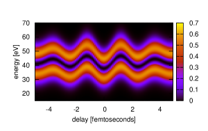
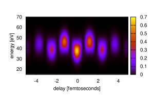
a) b)
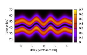
c) d)

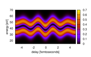
Figure 1: a) A streaking spectrogram calculated with the aid of Eq. (5) using a model transition matrix element (12). b) The spectrogram reconstructed using a FROG algorithm. c) The spectrogram calculated using the FROG ansatz (7) with the pulse $P_{1}(t)=\mathcal{E}_{\mathrm{XUV}}(t)$ and the gate $G_{1}(t)$. d) The FROG spectrogram evaluated with the pulse being the time-domain wave packet $\chi(t)$ and the gate $G_{2}(t)=\exp\{\mathrm{i}\Phi(\mathbf{p}_{0},t)\}$.

Fig. 1(a) shows a spectrogram calculated using Eq. (5). The FROG reconstruction Gagnon_APB_2008 yields a very similar spectrogram, Fig. 1(b). On the other hand, the conventional central momentum approximation, defined by Eqs. (7), (8), and (9), yields a spectrogram, shown in Fig. 1(c), which has very little resemblance to the original spectrogram. The approximation breaks down in this example because $D(p_{0})=0$. However, the pulse and gate pair given by Eqs. (10) and (11) yield a spectrogram that is very close to the original one: Fig. 1(d).

In Fig. 2, we compare the XUV envelope $\mathcal{E}_{\mathrm{XUV}}(t)$, the time-domain wave packet $\chi(t)$, and the pulse $P(t)$ retrieved by FROG from the spectrogram shown in Fig. 1(a). The retrieved pulse nearly coincides with the wave packet $\chi(t)$.

\psfrag{Figure2xlabel}{$t$ \footnotesize{[atomic units]}}\psfrag{Figure2ylabel}{\footnotesize{arb.\ units}}\psfrag{Figure2label1}[c]{$\mathcal{E}_{\mathrm{XUV}}(t)$}\psfrag{Figure2label2}[c]{$\operatorname{Im}[\chi(t)]$}\psfrag{Figure2label3}[c]{$\operatorname{Im}[P(t)]$}\includegraphics{Figure2.eps}

Figure 2: The envelope of the XUV pulse $\mathcal{E}_{\mathrm{XUV}}(t)$ (dash-dotted line), the time-domain wave packet $\chi(t)$ defined by Eq. (1) (solid line), and the pulse $P(t)$ retrieved by FROG from the spectrogram shown in Fig. 1(a) (diamonds). In this example, the real part of the wave packet is equal to zero, so we compare the imaginary parts of $\chi(t)$ and $P(t)$.

In the momentum space, we see that the wave packet and the retrieved pulse only differ in a narrow spectral region near the phase discontinuity, as shown in Fig. 3.

\psfrag{Figure3xlabel}{$p$ \footnotesize{[atomic units]}}\psfrag{Figure3ylabel}{\footnotesize{radians}}\psfrag{Figure3label1}[c]{$\mbox{arg}[\tilde{\chi}]$}\psfrag{Figure3label2}[c]{$\mbox{arg}[\tilde{P}]$}\includegraphics{Figure3.eps}

Figure 3: The phase of the momentum-space wave packet $\mbox{arg}[\tilde{\chi}(p)]$ (solid line) in comparison with the phase of the retrieved wave packet $\mbox{arg}\left[\tilde{P}\left(\frac{p^{2}}{2}-\frac{p_{0}^{2}}{2}\right)\right]$ (diamonds).

To gain insight as to why the time-domain wave packet $\eqref{eq:time_domain_WP}$ plays the role of the pulse, we use Eqs. (2) and (3) to express $\mathcal{E}_{\mathrm{XUV}}(t+\tau)$ in (5) via $\tilde{\chi}(p)$ and then expand $[D(p)]^{-1}$ in a Taylor series, which eventually allows us to rewrite the master equation (5) in a form where $\chi(t)$ plays the role of the pulse. In the case when the XUV and streaking pulses are polarized in the direction where photoelectrons are detected, $S(p,\tau)$ can be rewritten, without any approximations, as

$$S(p,\tau)=\left|\frac{1}{2}\int_{-\infty}^{\infty}dt\,\chi(t+\tau)\sum_{n=0}^{\infty}a_{n}\frac{\partial^{n}g(p,t)}{\partial t^{n}}\right|^{2},$$ (13)

where $a_{n}=\frac{(-i)^{n}}{n!}\left.{\frac{\partial^{n}}{\partial\omega^{n}}\frac{1}{D\left(\sqrt{2\omega+p_{0}^{2}}\right)}}\right|_{\omega=0}$ and

$$g(p,t)=D\bigl{(}p+A_{\mathrm{L}}(t)\bigr{)}e^{\mathrm{i}\Phi(p,t)+\mathrm{i}\left(\frac{p^{2}}{2}-\frac{p_{0}^{2}}{2}\right)t}.$$ (14)

Consequently, the FROG gate associated with the time-domain wave packet is given by

$$G_{2}(t)=\left.{\left(\sum_{n=0}^{\infty}a_{n}\frac{\partial^{n}g(p,t)}{\partial t^{n}}\right)}\right|_{p=p_{0}}.$$ (15)

Applying the central momentum approximation to Eq. (15), rather than Eq. (5), yields a spectrogram that is closer to the exact one. To show this analytically, we neglect all derivatives of $A_{\mathrm{L}}(t)$ in the expression for $\partial^{n}g(p,t)/\partial t^{n}$, which is justified if the exponential function in Eq. (14) oscillates with a period that is much shorter than the optical cycle of the streaking field. Once this approximation is made, we recognize that the sum over $n$ in Eq. (13) becomes the Taylor expansion of $[D\bigl{(}p+A_{\mathrm{L}}(t)\bigr{)}]^{-1}$, which simplifies Eq. (13) to

$$S(p,\tau)\approx\left|\frac{1}{2}\int_{-\infty}^{\infty}dt\,\chi(t+\tau)e^{\mathrm{i}\Phi(p,t)}e^{\mathrm{i}\left(\frac{p^{2}}{2}-\frac{p_{0}^{2}}{2}\right)t}\right|^{2}.$$ (16)

Thus, $G_{2}(t)\approx\exp\{\mathrm{i}\Phi(\mathbf{p}_{0},t)\}$. Importantly, the central momentum approximation applied this way does not affect the transition matrix element $D(p)$, while the conventional expression for the FROG gate (8) approximates $D(p+A_{\mathrm{L}}(t))$ with $D(p_{0}+A_{\mathrm{L}}(t))$. In the example presented above, this was a very poor approximation.

As a remark, we were able to find cases where Eq. (16) was a seemingly worse approximation to the true spectrogram (5) than the conventional central momentum approximation . Nevertheless, FROG retrieved the time-domain wave packet. This confirms that the central momentum approximation is more generally applicable if the spectrogram is expressed via $\chi(t)$ according to Eq. (13).

In conclusion, we have established that the time-domain wave packet $\chi(t)$ defined by Eq. (1) determines the output of attosecond streaking measurements processed with conventional retrieval algorithms, such as “frequency-resolved optical gating for complete reconstruction of attosecond bursts” (FROG CRAB) Mairesse_PRA_2005 . The analysis presented in this paper was focused on direct single-photon ionization with a complex transition matrix element, using a Cooper minimum as an example. However, it is known that Eq. (5) formally describes more sophisticated streaking measurements, such as those of the Fano resonances and autoionization decay Wickenhauser_PRL_2005 ; Zhao_PRA_2005 . Therefore, our analysis is directly applicable to these situations as well, Eq. (1) being a fundamental relation between the momentum-space wave function of a photoelectron and the pulse retrieved from a streaking spectrogram.

Having established this relation, we claim that the quantum phase associated with bound-free transitions can be measured (up to a constant phase) by means of attosecond streaking. According to Eq. (2), this is possible if the spectral phase of an attosecond pulse is known. An XUV pulse can be fully characterized in a streaking measurement performed on an atom where the accurate matrix elements are known from a reliable model or their phases are known to be negligible. For example, helium can be used for such a calibration. Then another streaking measurement on the system under scrutiny will provide all the necessary information to retrieve the unknown phases of quantum transitions and thus completely characterize photoionization dynamics. Such a measurement would be a test and, possibly, a challenge for many-electron theories of photoionization, especially if the ionization involves a resonance state or a Cooper minimum.

- (1) M. Drescher, M. Hentschel, R. Kienberger, M. Uiberacker, V. Yakovlev, A. Scrinzi, T. Westerwalbesloh, U. Kleineberg, U. Heinzmann, and F. Krausz, Nature 419, 803 (Oct 24 2002)
- (2) M. Swoboda, T. Fordell, K. Klünder, J. M. Dahlström, M. Miranda, C. Buth, K. J. Schafer, J. Mauritsson, A. L’Huillier, and M. Gisselbrecht, Phys. Rev. Lett. 104, 103003 (Mar 2010)
- (3) M. Schultze, M. Fieß, N. Karpowicz, J. Gagnon, M. Korbman, M. Hofstetter, S. Neppl, A. L. Cavalieri, Y. Komninos, T. Mercouris, C. A. Nicolaides, R. Pazourek, S. Nagele, J. Feist, J. Burgdörfer, A. M. Azzeer, R. Ernstorfer, R. Kienberger, U. Kleineberg, E. Goulielmakis, F. Krausz, and V. S. Yakovlev, Science 328, 1658 (Jun 25 2010)
- (4) J. Itatani, F. Quéré, G. L. Yudin, M. Y. Ivanov, F. Krausz, and P. B. Corkum, Phys. Rev. Lett. 88, 173903 (Apr 2002)
- (5) M. Kitzler, N. Milosevic, A. Scrinzi, F. Krausz, and T. Brabec, Phys. Rev. Lett. 88, 173904 (Apr 2002)
- (6) R. Kienberger, E. Goulielmakis, M. Uiberacker, A. Baltuska, V. Yakovlev, F. Bammer, A. Scrinzi, T. Westerwalbesloh, U. Kleineberg, U. Heinzmann, M. Drescher, and F. Krausz, Nature 427, 817 (Feb 26 2004)
- (7) F. Quere, Y. Mairesse, and J. Itatani, J. Mod. Opt. 52, 339 (Jan-Feb 2005)
- (8) J. Gagnon, E. Goulielmakis, and V. S. Yakovlev, Appl. Phys. B 92, 25 (Jul 2008)
- (9) J. Gagnon and V. S. Yakovlev, Opt. Expr. 17, 17678 (Sep 28 2009)
- (10) J. Mauritsson, M. B. Gaarde, and K. J. Schafer, Phys. Rev. A 72, 013401 (Jul 2005)
- (11) G. L. Yudin, S. Patchkovskii, and A. D. Bandrauk, J. Phys. B 41, 045602 (Feb 28 2008)
- (12) A. S. Kornev and B. A. Zon, J. of Phys. B 35, 2451 (2002)
- (13) Y. Mairesse and F. Quéré, Phys. Rev. A 71, 011401(R) (Jan 2005)
- (14) In the literature on frequency-resolved optical gating, is usually referred to as “probe”.
- (15) R. Trebino, K. W. DeLong, D. N. Fittinghoff, J. N. Sweetser, M. A. Krumbugel, B. A. Richman, and D. J. Kane, Rev. Scient. Instr. 68, 3277 (Sep 1997)
- (16) D. J. Kane, IEEE J. Quant. Electron. 35, 421 (Apr 1999), ISSN 0018-9197
- (17) G. Sansone, E. Benedetti, F. Calegari, C. Vozzi, L. Avaldi, R. Flammini, L. Poletto, P. Villoresi, C. Altucci, R. Velotta, S. Stagira, S. De Silvestri, and M. Nisoli, Science 314, 443 (Oct 20 2006)
- (18) J. W. Cooper, Phys. Rev. 128, 681 (Oct 1962)
- (19) For example, if we use instead of Eq. (2\@@italiccorr).
- (20) M. Wickenhauser, J. Burgdörfer, F. Krausz, and M. Drescher, Phys. Rev. Lett. 94, 023002 (Jan 2005)
- (21) Z. X. Zhao and C. D. Lin, Phys. Rev. A 71, 060702(R) (Jun 2005)