6.1mm

Random Numbers in Scientific Computing:
An Introduction

Helmut G. Katzgraber

Department of Physics and Astronomy, Texas A&M University
College Station, Texas 77843-4242 USA
Theoretische Physik, ETH Zurich
CH-8093 Zurich, Switzerland

Abstract.

Random numbers play a crucial role in science and industry. Many numerical methods require the use of random numbers, in particular the Monte Carlo method. Therefore it is of paramount importance to have efficient random number generators. The differences, advantages and disadvantages of true and pseudo random number generators are discussed with an emphasis on the intrinsic details of modern and fast pseudo random number generators. Furthermore, standard tests to verify the quality of the random numbers produced by a given generator are outlined. Finally, standard scientific libraries with built-in generators are presented, as well as different approaches to generate nonuniform random numbers. Potential problems that one might encounter when using large parallel machines are discussed.

1 Introduction

Random numbers are of paramount importance. Not only are they needed for gambling, they find applications in cryptography, statistical data sampling, as well as computer simulation (e.g., Monte Carlo simulations). In principle, they are needed in any application where unpredictable results are required. For most applications it is desirable to have fast random number generators (RNGs) that produce numbers that are as random as possible. However, these two properties are often inversely proportional to each other: excellent RNGs are often slow, whereas poor RNGs are typically fast.

In times where computers can easily perform $10^{9}$ operations per second, vast amounts of uncorrelated random numbers have to be produced quickly. For this purpose, pseudo random number generators (PRNGs) have been developed. However, for “mission-critical” applications (e.g., data encryption) true random number generators (TRNGs) should be used. Both TRNGs and PRNGs have pros and cons which are outlined below.

The goal of this tutorial is to present an overview of the different types of random number generators, their advantages and disadvantages, as well as how to test the quality of a generator. There will be no rigorous proofs. For a detailed mathematical treatment, the reader is referred to Refs. [14] and [16]. In addition, methods to produce random numbers beyond uniform distributions are presented. Finally, some well-tested RNG implementations in scientific libraries are outlined.

The list of highlighted generators is by no means complete and some readers might find that their generator of choice is probably not even mentioned. There are many ways to produce pseudo random numbers. In this tutorial we mainly mention those generators that have passed common PRNG quality benchmarks and are fast. If you find yourself using one of the bad generators outlined here, I highly recommend you switch to one of the good generator mentioned below.

2 True random number generators (TRNGs)

TRNGs generally use some physical process that is unpredictable, combined with some compensation mechanism that might remove any bias in the process.

For example, the possibly oldest TRNG is coin tossing. Assuming that the coin is perfectly symmetric, one can expect that both head or tail will appear 50% of the time (on average). This means that “random bits” $0$ (head) and $1$ (tail) can thus be generated and grouped into blocks that then can be used to produce, for example, integers of a given size (for example, 32 coin tosses can be used to produce a 32-bit integer). If, however, the coin is not symmetric, head might occur 45% of the time, whereas tail might occur 55% of the time (and if you are really unlucky, the coin will land on the edge …). In such cases, post-processing corrections must be applied to ensure that the numbers are truly random and unbiased. TRNGs have typically the following advantages:

• True random numbers are generated.

• There are no correlations in the sequence of numbers – assuming proper biasing compensation is performed.

However, the fact that we are dealing with true random numbers, also has its disadvantages:

• TRNGs are generally slow and therefore only of limited use for large-scale computer simulations that require large amounts of random numbers.

• Because the numbers are truly random, debugging of a program can be difficult. PRNGs on the other hand can produce the exact same sequence of numbers if needed, thus facilitating debugging.

TRNGs are generally used for cryptographic applications, seeding of large-scale simulations, as well as any application that needs few but true random numbers. Selected implementations:

• Early approaches: coin flipping, rolling of dice, roulette. These, however, are pretty slow for most applications.

• Devices that use physical processes that are inherently random, such as radioactive decays, thermal noise, atmospheric radio noise, shot noise, etc.

• Quantum processes: idQuantique [1] produces hardware quantum random number generators using quantum optics processes. Photons are sent onto a semi-transparent mirror. Part of the photons are reflected and some are transmitted in an unpredictable way (the wonders of quantum mechanics…). The transmitted/reflected photons are subsequently detected and associated with random bits $0$ and $1$.

• Human game-play entropy: The behavior of human players in massive multiplayer online (MMO) games is unpredictable. There have been proposals to use this game entropy to generate true random numbers.

• More imaginative approaches: Silicon Graphics produced a TRNG based on a lava lamp. Called “LavaRand,” the hardware would take images from the lava blobs inside a lava lamp. The randomness is then extracted from the random shapes on the images and used to seed a PRNG.

• /dev/random/: In Unix operating systems /dev/random/ is a source of randomness based on noise collected from device drivers. Note that /dev/random/ is not necessarily a TRNG. However, for the Linux operating system this is generally the case, although it has been shown that the produced random numbers can have correlations when certain devices are used for entropy gathering. Note that /dev/urandom/ is an “unblocked” version where the output is faster, but which might contain less entropy, i.e., lower-quality random numbers.

3 Pseudo random number generators (PRNGs)

PRNGs are based on algorithms. Therefore, PRNGs are deterministic and not truly random. Advantages are:

• Random number generation is fast (no need for post-processing).

• PRNGs do not require special hardware and therefore are very portable.

• If needed, the exact sequence of seemingly random numbers can be reproduced, e.g., for debugging purposes.

The fact that good pseudo random numbers can be generated quickly makes PRNGs the typical choice for scientific applications, as well as statistical data analysis and noncritical applications (think of Unix’s motd). However, the aforementioned advantages come at a price:

• PRNGs have finite sequence lengths. At some point, the numbers repeat. In large-scale simulations where many random numbers are needed it is imperative to choose a good generator with an astronomically large period [2].

• The numbers produced by a PRNG can be correlated. In particular, grouping the numbers in certain ways might produce correlations that are otherwise invisible. Therefore, thorough tests (discussed later) need to be performed before a PRNG is used in a scientific application.

The idea behind an algorithmic PRNG is to generate a sequence of numbers $x_{1}$, $x_{2}$, $x_{3}$, …using a recurrence of the form

$$x_{i}=f(x_{i-1},x_{i-2},\ldots,x_{i-n})\,,$$ (1)

where $n$ initial numbers (seed block) are needed to start the recurrence. All PRNGs have the structure shown in Eq. (1), the magic lies in finding a function $f$ that produces numbers that are “as random as possible.” Some PRNGs use the modulo operation to further randomize the numbers. This has the effect that often the maximum sequence length is limited.

The seed determines the sequence of random numbers. Therefore, it is crucial to seed the PRNG carefully. For example, if the period of the PRNG is rather short, repeated seeding might produce overlapping streams of random numbers. Furthermore, there are generators where a poor choice of the seed might produce correlated random numbers. So …which generator should one use? In what follows, some typical PRNGs are discussed and outlined.

3.1 Linear congruential generators

Linear congruential generators (LCGs) are one of the oldest PRNGs. In their simplest implementation, they are of the form [11]

$$x_{i+1}=(ax_{i}+c)\bmod m$$ (2)

with $x_{0}$ a seed value. In Eq. (2) $m$ is a large integer that determines the period of the generator; it will thus produce numbers between $0$ and $m-1$. Note that this is similar to a roulette where a croupier spins a wheel with $37$ pockets in one direction, then spins a ball in the opposite direction around a tilted circular track running around the circumference of the wheel. The ball eventually slows down and lands in one of the $m=37$ pockets. $0\leq a<m$ is called the multiplier and $0\leq c<m$ is the increment. The case where $c=0$ corresponds to the Park-Miller PRNG. The values of $a$, $c$, $x_{0}$ and $m$ can heavily influence the behavior of the LCG. One can rigorously show that a LCG has period $m$ if and only if $c$ is relatively prime to $m$, $a-1$ is a multiple of $p$ for every prime $p$ dividing $m$, and $a-1$ is a multiple of $4$, if $m$ is a multiple of $4$. Dizzy yet? An acceptable choice is given by the GGL generator where $a=16807$, $c=0$ and $m=2^{31}-1$. An example of a bad generator is given below.

A more general approach is used in linear feedback shift register generators given by the following recurrence (with $c=0$) [15]

$$x_{i}=(a_{1}x_{i-1}+a_{2}x_{i-2}+\ldots+a_{n}x_{i-n})\bmod p\,.$$ (3)

Here $p$ is a prime number. The quality of the pseudo random numbers depends on the multipliers $a_{k}$, as well as $n$ and $p$. One can show that the maximum period of such a generator is $p^{n}-1$. However, if the parameters of the generator are not chosen carefully, the period can be considerably shorter than the maximum period. The period is maximal if and only if the characteristic polynomial

$$f(x)=x^{n}-a_{1}x^{n-1}-a_{2}x^{n-2}-\ldots-a_{n}$$ (4)

is primitive modulo $p$.

LCGs are extremely fast and use little memory, however, the period is limited by the choice of $m$. For standard LCGs, $m\sim 2^{32}$ which corresponds to approximately $10^{9}$ random numbers. On a modern computer such a sequence is exhausted in seconds. If $m=2^{k}$ ($k\in{\mathbb{N}}$) then lower-order bits of the generated sequence have a far shorter period than the sequence as a whole. Therefore never use a linear congruential PRNG for numerical simulations. However, it is acceptable to use a LCG to generate a seed block for a more complex PRNG. Finally, note that LCGs are difficult to parallelize.

Example of a bad generator: RANDU

RANDU is a linear congruential PRNG of the Park-Miller type that was installed as the standard generator on IBM mainframe computers in the 1960s. It uses the parameters $a=65539$, $c=0$, and $m=2^{31}$. The particular choice of $a=65539=2^{16}+3$ was made to speed up the modulo operation on 32-bit machines. The fact that the numbers have correlations can be illustrated with the following simple calculation (modulo $m$ means that $2^{32}\equiv 0$)

$$x_{i+2} = ax_{i+1}=(2^{16}+3)x_{i+1}=(2^{16}+3)^{2}x_{i}$$

$$= (2^{32}+6\cdot 2^{16}+9)x_{i}\equiv[6(2^{16}+3)-9]x_{i}$$

$$= 6x_{i+1}-9x_{i}\,.$$

Therefore, tuplets of random numbers have to be correlated. If three consecutive random numbers $x_{1}$, $x_{2}$ and $x_{3}$ are combined to a vector $(x_{1},x_{2},x_{3})$, then the numbers lie on planes in three-dimensional space, as can be seen in Fig. 1.

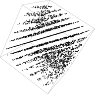
Figure 1: $10^{3}$ triplets of successive random numbers produced with RANDU plotted in three-dimensional space. If the random numbers were perfectly random, no planes should be visible. However, when viewed from the right angle, planes emerge, thus showing that the random numbers are strongly correlated.

3.2 Lagged Fibonacci generators

Lagged Fibonacci generators are intended as an improvement over linear congruential generators and, in general, they are not only fast but most of them pass all standard empirical random number generator tests. The name comes from the similarity to the Fibonacci series

$$x_{i}=x_{i-1}+x_{i-2}\;\;\;\longrightarrow\;\;\;\{1,1,2,3,5,8,13,21,\ldots\}$$ (6)

with $x_{0}=x_{1}=1$. In this case we generalize Eq. (6) to the following sequence

$$x_{i}=(x_{i-j}\odot x_{i-k})\bmod m\,,\;\;\;\;\;\;\;\;\;\;\;0<j<k,$$ (7)

where $\odot$ represents a binary operator, i.e., addition, multiplication or exclusive OR (XOR). Typically $m=2^{M}$ with $M=32$ or $64$. Generators of this type require a seed block of size $k$ to be initialized. In general, one uses a very good yet possibly slow [e.g., ran2( ), see below] PRNG to build the seed block. When the operator is a multiplication [addition] the PRNG is called a multiplicative [additive] lagged Fibonacci generator. The case where the operator is XOR is known as two-tap generalised feedback shift register (GFSR). Note that the Mersenne Twister (discussed below in Sec. 3.3) is a variation of a GFSR. In fact, the linear and generalized shift register generators, the Mersenne Twister and the WELL PRNG (see below) belong to a class of generators known as ${\mathbb{F}}_{2}$-linear PRNGs because they are based on a recurrence over a finite binary field ${\mathbb{F}}_{2}$.

The theory behind this class of generators is rather complex and there are no rigorous proofs on the performance of these generators. Therefore their quality relies vastly on statistical tests. In particular, they are very sensitive to initialization, which is why a very good generator has to be used to build the seed block. Furthermore, the values of $j$ and $k$ have to be chosen carefully. For the generator to achieve the maximum period, the polynomial

$$y=x^{k}+x^{j}+1$$ (8)

must be primitive over the integers modulo 2. Some commonly-used choices for 64-bit additive generators are the following pairs: $\{55,24,\oplus\}$, $\{607,273,\oplus\}$, $\{2281,1252,\oplus\}$, $\{9689,5502,\oplus\}$. For multiplicative generators common values are $\{1279,418,\otimes\}$ and $\{250,103,\otimes\}$. Note that, in general, the larger the values of the lags, the better the generator. Furthermore, the length of the period $\rho$ depends on $m=2^{M}$ and $k$. For example:

$$\rho(\oplus)=2^{k-1}2^{M-1},\;\;\;\;\;\;\;\;\;\;\;\;\;\;\;\;\;\;\;\;\;\;\;\;\;\;\;\;\;\rho(\otimes)=2^{k-1}2^{M-3}\,.$$ (9)

Lagged Fibonacci generators are thus fast, generally pass all known statistical quality tests and have very long periods. They can also be vectorized on vector CPU computers, as well as pipelined on scalar CPUs.

Example of a commonly-used good generator: r1279

In the case of r1279( ) with 32 bits—a multiplicative generator with $k=1279$—the period is approximately $10^{394}$, a very large number if you compare to linear congruential generators. r1279( ) passes all known RNG tests. Furthermore, there are fast implementations. Therefore, it is one of the RNGs of choice in numerical simulations, which is why it is standard in many scientific computing libraries, such as the GSL [3].

Example of a bad generator: r250

For many years r250( ) ($k=250$, $\odot={\rm XOR}$) was the standard generator in numerical simulations. Not only was it fast, it passed all common RNG quality tests at that time. However, in 1992 Ferrenberg et al. performed a Monte Carlo simulation of the two-dimensional Ising model [13, 12] using the Wolff cluster algorithm [17]. Surprisingly, the estimate of the energy per spin at the critical temperature was approximately $42$ standard deviations off the known exact result. After many tests they concluded that the random number generator used, namely r250( ) was the culprit. This case illustrates that although a generator passes all known statistical tests, there is no guarantee that the produced numbers are random enough.

3.3 Other commonly-used PRNGs

Mersenne Twister

The Mersenne Twister was developed in 1997 by Matsumoto and Nishimura and is a version of a generalised feedback shift register PRNG. The name comes from the fact that the period is given by a Mersenne prime ($M_{n}=2^{n}-1$, $n\in{\mathbb{N}}$). It is very fast and produces high-quality random numbers. The implementation mt19937( ), which is part of many languages and scientific libraries such as Matlab, R, Python, Boost [4] or the GSL [3], has a period of $\rho=2^{19937}-1\approx 10^{6001}$. There are two common versions of mt19937( ) for 32 and 64-bit architectures. For a $k$-bit word length, the Mersenne Twister generates numbers with a uniform distribution in the range $[0,2^{k}-1]$. Although the Mersenne Twister can be checkpointed easily, it is based on a rather complex algorithm.

WELL generators

The name stands for Well Equidistributed Long-period Linear. The idea behind the generator originally developed by Panneton, L’Ecuyer and Matsumoto is to provide better equidistribution and bit mixing with an equivalent period length and speed as the Mersenne Twister.

ran2

The Numerical Recipes [16] offers different random number generators. Do not use the quick-and-dirty generators for mission critical applications. They are quick, but dirty (and thus bad). Both ran0( ) and ran1( ) are not recommended either since they do not pass all statistical tests and have short periods of $2^{32}$. ran2( ), however, has a period of $\sim 10^{18}$ (still modest in comparison to other generators outlined here) and passes all statistical tests. In fact, the authors of the Numerical Recipes are willing to pay $1000 to the first person who proves that ran2( ) fails a statistical test. Note that ran2( ) is rather slow and should only be used to generate seed blocks for better generators.

drand48

The Unix built-in family of generators drand48( ) is actually based on a linear congruential generator with a 48-bit integer arithmetic. Pseudo random numbers are generated according to Eq. (2) with $a=25214903917$, $c=11$ and $m=2^{48}$. Clearly, this generator should not be used for numerical simulations. Not only is the maximal period only $\sim 10^{14}$, linear congruential generators are known to have correlation effects.

Online services

A website that delivers true random numbers is random.org. Although not very useful for large-scale simulations, the site delivers true random numbers (using atmospheric noise). There is a limit of free random bits. In general, the service costs approximately US$ 1 per 4 million random bits. A large-scale Monte Carlo simulation with $10^{12}$ random numbers would therefore cost US$ 250,000.

Final recommendation

For any scientific applications avoid the use of linear congruential generators, the family of Unix built-in generators drand48( ), Numerical Recipe’s ran0( ), ran1( ) and ran2( ), as well as any home-cooked routines. Instead, use either a multiplicative lagged Fibonacci generator such as r1279( ), WELL generators, or the Mersenne Twister. Not only are they good, they are very fast.

4 Testing the quality of random number generators

In the previous chapters we have talked about “good” and “bad” generators mentioning often “statistical tests.” There are obvious reasons why a PRNG might be bad: For example, with a period of $10^{9}$ a generator is useless for most scientific applications. As in the case of r250( ) [10], there can be very subtle effects that might bias data in a simulation. These subtle effects can often only be discovered by performing batteries of statistical tests that try to find hidden correlations in the stream of random numbers. In the end, our goal is to obtain pseudo random numbers that are like true random numbers.

Over the years many empirical statistical tests have been developed that attempt to determine if there are any short-time or long-time correlations between the numbers, as well as their distribution. Are these tests enough? No. As in the case of r250( ), your simulation could depend in a subtle way on hidden correlations. What is thus the ultimate test? Run your code with different PRNGs. If the results agree within error bars and the PRNGs used are from different families, the results are likely to be correct.

4.1 Simple PRNG tests

If your PRNG does not pass the following tests, then you should definitely not use it. The tests are based on the fact that if one assumes that the produced random numbers have no correlations, the error should be purely statistical and scale as $1/\sqrt{N}$ where $N$ is the number of random numbers used for the test.

Simple correlations test

For all $n\in{\mathbb{N}}$ calculate the following function

$$\varepsilon(N,n)=\frac{1}{N}\sum_{i=1}^{N}x_{i}x_{i+n}-E(x)^{2}\,,$$ (10)

where

$$E(x)=\frac{1}{N}\sum_{i=1}^{N}x_{i}$$ (11)

represents the average over the sampled pseudo random numbers. If the tuplets of numbers are not correlated, $\varepsilon(N,n)$ should converge to zero with a statistical error for $N\to\infty$, i.e.,

$$\varepsilon(N,n)\sim{\mathcal{O}}(N^{-1/2})\;\;\;\;\;\;\;\;\;\forall n\;.$$ (12)

Simple moments test

Let us assume that the PRNG to be tested produces uniform pseudo random numbers in the interval $[0,1]$. One can analytically show that for a uniform distribution the $k$-th moment is given by $1/(k+1)$. One can therefore calculate the following function for the $k$th moment

$$\mu(N,k)=\left|\frac{1}{N}\sum_{i=1}^{N}x_{i}^{k}-\frac{1}{k+1}\right|\;.$$ (13)

Again, for $N\to\infty$

$$\mu(N,k)\sim{\mathcal{O}}(N^{-1/2})\;\;\;\;\;\;\;\;\;\forall k\;.$$ (14)

Graphical tests

Another simple test to look for “spatial correlations” is to group a stream of pseudo random numbers into $k$-tuplets. These tests are also known under the name “spectral tests.” For example, a stream of numbers $x_{1}$, $x_{2}$, …can be used to produce two-dimensional vectors $\vec{v}_{1}=(x_{1},x_{2})$, $\vec{v}_{2}=(x_{3},x_{4})$, …, as well as three-dimensional or normalized unit vectors ($\vec{e}=\vec{x}/||\vec{x}||$). Figure 2 shows data for 2-tuplets and normalized 3-tuplets for both good and bad PRNGs. While the good PRNG shows no clear sign of correlations, these are evident in the bad PRNG.

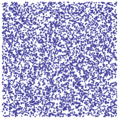
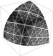
Figure 2: Graphical correlations test using a home-cooked linear congruential generator with $a=106$, $c=1283$ and $m=6075$ (left panels) and the Mersenne Twister (right panels). The top row shows 2-tuplets in the plane. Correlations (left-hand-side) are clearly visible for the home-cooked PRNG. The bottom row shows 3-tuplets on the unit sphere. Again, the home-cooked PRNG (left-hand-side), albeit pretty, shows extreme correlations.

Theoretical details on spectral tests, as well as many other methods to test the quality of PRNGs such as the chi-squared test, can be found in Ref. [14].

4.2 Test suites

There are different test suites that have been developed with the sole purpose of testing PRNGs. In general, it is recommended to use these to test a new generator as they are well established. Probably the oldest and most commonly used test suite is DIEHARD by George Marsaglia.

DIEHARD

The software is freely available [5] and comprises 16 standard tests. Most of the tests in DIEHARD return a $p$-value, which should be uniform on the interval $[0,1)$ if the pseudo random numbers are truly independent random bits. When a bit stream fails the test, $p$-values near 0 or 1 to six or more digits are obtained (for details see Refs. [5] and [14]). DIEHARD includes the following tests (selection):

• Overlapping permutations test: Analyze sequences of five consecutive random numbers. The $5!=120$ possible permutations should occur (statistically) with equal probability.

• Birthday spacings test: Choose random points on a large interval. The spacings between the points should be asymptotically Poisson-distributed.

• Binary rank test for $32\times 32$ matrices: A random $32\times 32$ binary matrix is formed. The rank is determined, it can be between 0 and 32. Ranks less than 29 are rare, and so their counts are pooled with those of 29. Ranks are found for $40\,000$ random matrices and a chi-square test [14] is performed for ranks 32, 31, 30, and $\leq 29$.

• Parking lot test: Randomly place unit circles in a $100\times 100$ square. If the circle overlaps an existing one, choose a new position until the circle does not overlap. After $12\,000$ attempts, the number of successfully “parked” circles should follow a certain normal distribution.

It is beyond the scope of this lecture to outline all tests. In general, the DIEHARD tests perform operations on random number streams that in the end should be either distributed according to a given distribution that can be computed analytically, or the problem is reduced to a case where a chi-square or Kolmogorov-Smirnov test [14] can be applied to measure the quality of the random series.

NIST test suite

The US National Institute of Standards and Technology (NIST) has also published a PRNG test suite [6]. It can be downloaded freely from their website. The test suite contains 15 tests that are extremely well documented. The software is available for many architectures and operating systems and considerably more up-to-date than DIEHARD. Quite a few of the tests are from the DIEHARD test suite, however, some are novel tests that very nicely test the properties of PRNGs.

L’Ecuyer’s test suite

Pierre L’Ecuyer has not only developed different PRNGs, he has also designed TestU01, a ANSI C software library of utilities for the empirical statistical testing of PRNGs [7]. In addition, the library implements several PRNGs and is very well documented.

5 Nonuniform random numbers

Standard random number generators typically produce either bit streams, uniform random integers between 0 and INT_MAX, or floating-point numbers in the interval $[0,1)$. However, in many applications it is desirable to have random numbers distributed according to a probability distribution that is not uniform. In this section different approaches to generate nonuniform random numbers are presented.

5.1 Binary to decimal

Some generators merely produce streams of binary bits. Using the relation

$$u=\sum_{i=0}^{B}b_{i}2^{i}$$ (15)

integers $x$ between $0$ and $2^{B}$ can be produced. The bit stream $b_{i}$ is buffered into blocks of $B$ bits and from there an integer is constructed. If floating-point random numbers in the interval $[0,1)$ are needed, we need to replace $u\to u/2^{B}$.

5.2 Arbitrary uniform random numbers

Uniform random numbers $r$ in the interval $[a,b)$ can be computed by a simple linear transformation starting from uniformly distributed random numbers $u\in[0,1)$

$$r=a+(b-a)u\,.$$ (16)

More complex transformations need the help of probability theory.

5.3 Transformation method

The probability $p(u)du$ of generating a uniform random number between $u$ and $u+du$ is given by

$$p(u)du=\left\{\begin{array}[]{rl}du&0<u<1\\ 0&\mbox{ otherwise}\,.\end{array}\right.$$ (17)

Note that the probability distribution is normalized, i.e.,

$$\int_{-\infty}^{\infty}p(u)du=1\,.$$ (18)

Suppose we take a prescribed function $y(u)$ of a uniform random number $u$. The probability distribution of $y$, $q(y)dy$, is determined by the transformation law of probabilities, namely [11]

$$|q(y)dy|=|p(u)du|\longrightarrow q(y)=p(u)\left|\frac{du}{dy}\right|\,.$$ (19)

If we can invert the function, we can compute nonuniform deviates.

5.4 Exponential deviates

To compute exponentially-distributed random numbers with

$$q(y)=a\exp(-ay)$$ (20)

we use Eq. (19):

$$\left|\frac{du}{dy}\right|=a\exp(-ay)\longrightarrow u(y)=\exp(-ay)\,.$$ (21)

Inverting Eq. (21) we obtain for exponentially-distributed random numbers

$$y=-\frac{1}{a}\ln(u)\,,$$ (22)

where $u\to 1-u\in(0,1]$ is a uniform random number.

5.5 Gaussian-distributed random numbers

Gaussian-distributed (also known as Normal) random numbers find wide applicability in many computational problems. It is therefore desirable to efficiently compute these. The probability distribution function is given by

$$q(y)=\frac{1}{\sqrt{2\pi}}\exp(-y^{2}/2)\,.$$ (23)

The most widespread approach to generate Gaussian-distributed random numbers is the Box-Muller method: The transformation presented in Sec. 5.3 can be generalized to higher space dimensions. In one space dimension, it is not possible to solve the integral and therefore invert the function. However, in two space dimensions this is possible:

$$q(x)q(y)dxdy=\frac{1}{2\pi}e^{-(x^{2}+y^{2})/2}dxdy=\frac{1}{2\pi}e^{-R^{2}/2}RdRd\theta\to e^{-t}dt\,.$$ (24)

Let $u_{1}$ and $u_{2}$ be two uniform random numbers. Then

$$\theta=2\pi u_{1},\;\;\;\;\;\;\;\;\;\;\;\;\;\;\;\;\;\;\;t=-\ln(u_{2})\,.$$ (25)

It follows that

$$R=\sqrt{-2\ln(u_{2})}$$ (26)

and therefore

$$x = \sqrt{-2\ln(u_{2})}\cos(2\pi u_{1}),$$ (27)

$$y = \sqrt{-2\ln(u_{2})}\sin(2\pi u_{1})\,.$$

At each step of the algorithm two uniform random numbers are converted into two Gaussian-distributed random numbers. Using simple rejection methods one can speed up the algorithm by preventing the use of trigonometric functions in Eqs. (27). For details see Ref. [16].

5.6 Acceptance-Rejection method

When the integral in the transformation method (Sec. 5.3) cannot be inverted easily one can apply the acceptance-rejection method, provided that the distribution function $f(x)$ for the random numbers is known and computable. The idea behind the acceptance-rejection method is simple: Find a distribution function $g(x)$ that bounds $f(x)$ over a finite interval (and for which one can easily compute random numbers):

$$f(x)\leq g(x)\,.$$ (28)

The algorithm is simple [11]:

1 repeat2     generate a g-distributed random number x from g(x)3     generate a uniform random number u in [0,1]4 until5     u < f(x)/g(x)6 done78 return x

Basically, one produces a point in the two-dimensional plane under the function $g(x)$, see Fig. 3. If the point lies under the function $f(x)$ it is accepted as an $f$-distributed random number (light shaded area in Fig. 3). If it lies in the dark shaded area of Fig. 3 it is rejected. Note that this is very similar to Monte Carlo integration: The number of rejected points depends on the ratio between the area of $g(x)$ to the area of $f(x)$. Therefore, it is imperative to have a good guess for the function $g(x)$ that…

• is as close as possible to $f(x)$ to prevent many rejected moves.

• is quickly evaluated.

For very complex cases numerical inversion of the function $f(x)$ might be faster.

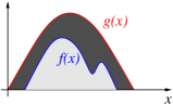
Figure 3: Illustration of the rejection method. If the point $(u,g(x))$ lies in the light shaded area, it is $f$-distributed. If it lies in the dark shaded area it is rejected.

5.7 Random numbers on a $N$-sphere

Sometimes it is necessary to generate random number on a $N$-sphere. There are two possible approaches:

• Using the Box-Muller method (Sec. 5.5):

  • Start from a uniform random vector $\vec{u}$.

  • Use the Box-Muller method on each component to obtain a normally-distributed vector $\vec{n}$.

  • Normalize the length of the vector to unity: $\vec{e}=\vec{n}/||\vec{n}||$. The angles are now uniformly distributed.

• Using Acceptance-Rejection:

  • Generate a uniform random vector $\vec{u}$ with each component in the interval $[-1,1]$.

  • If $||\vec{u}||>1$, choose a new vector.

  • Otherwise normalize the length of $\vec{u}\to\vec{u}/||\vec{u}||$.

The second approach using the acceptance-rejection method works better if $N$ is small.

6 Library implementations of PRNGs

It is not recommended to implement one’s own PRNG, especially because there are different well-tested libraries that contain most of the common generators. In addition, these routines are highly optimized, which is very important. For example, in a Monte Carlo simulation the PRNG is the most called function (at least 80% of the time). Therefore it is crucial to have a fast implementation. Standard libraries that contain PRNGs are

• Boost Libraries [4]: Generic implementation of many PRNGs in C++.

• GSL (Gnu Scientific Library) [3]: Efficient implementation of a vast selection of PRNGs in C with checkpointing built in.

• TRNG [8]: Implementation of different PRNGs with checkpointing built in. The library is designed with large-scale parallel simulations in mind, i.e., block splitting and leapfrogging are also implemented [9, 15].

• Numerical Recipes [16]: Implementation of some PRNGs. The libraries, however, are dated and the license restrictions ridiculous.

In what follows some details on how to use random number generators on both the GSL and Boost libraries are outlined. Note that these libraries are built in a modular way. They contain:

• (Uniform) Pseudo random number generator engines (e.g., Mersenne Twister, LCGs, Lagged Fibonacci generators, …).

• Distribution functions (e.g., Gaussian, Gamma, Poisson, Binomial, …).

• Tests.

6.1 Boost

The C++ Boost libraries [4] contain several PRNGs outlined in these lecture notes. For example, one can define a PRNG rng1 that produces random numbers using the Mersenne Twister, a rng2 that produces random numbers using a lagged Fibonacci generator, or rng3 using a LCG with the following lines of code:

 boost::mt19937 rng1;                   // mersenne twister
 boost::lagged_fibonacci1279 rng2;      // lagged fibonacci r1279
 boost::minstd_rand0 rng3;              // linear congruential

These can now be combined with different distribution functions. The uniform distributions in an interval $[a,b]$ can be called with

 boost::uniform_int<int> dist1(a,b);     // integers between a and b
 boost::uniform_real<double> dist2(a,b); // doubles between a and b

There are many more distribution functions and the reader is referred to the documentation [4]. For example

 boost::exponential_distribution<double> dist3(a);

produces random numbers with the distribution shown in Eq. (20). Gaussian random numbers [Eq. (23)] can be produced with

 boost::normal_distribution<double> dist4(mu,sigma);

where mu is the mean of the distribution and sigma its width. Combining generators and distributions can be accomplished with boost::variate_generator. For example, to produce 100 uniform random numbers in the interval $[0,1)$ using the Mersenne Twister:

1  #include <boost/random.hpp> 2 3  int main (void) 4  { 5 6  // define distribution 7  boost::uniform_real<double> dist(0.,1.); 8 9  // define the PRNG engine 10  boost::mt19937 engine; 11 12  // create a normally-distributed generator 13  boost::variate_generator<boost::mt19937&, 14      boost::normal_distribution<double> > 15      rng(engine,dist); 16 17   // seed it 18   engine.seed(1234u); 19 20  // use it 21  for (int i = 0; i < 100; i++){ 22      std::cout << rng() << "\n"; 23  }

For further details consult the Boost documentation [4].

6.2 GSL

The GSL is similar to the Boost libraries. One can define both PRNG engines and distributions and combine these to produce pretty much any kind of random number. For example, to produce 100 uniform random numbers in the interval $[0,1)$ using the Mersenne Twister:

1  #include <stdio.h> 2  #include <gsl/gsl_rng.h> 3 4  int main() 5  { 6      gsl_rng *rng;                             /* pointer to RNG */ 7      int    i;                                       /* iterator */ 8      double u;                                  /* random number */ 9 10      rng = gsl_rng_alloc(gsl_rng_mt19937); /* allocate generator */ 11      gsl_rng_set(rng,1234)                 /* seed the generator */ 12 13      for(i = 0; i < 100; i++){ 14          u = gsl_rng_uniform(rng);    /* generate random numbers */ 15          printf("%f\n", u); 16      } 17 18      gsl_rng_free(rng);                      /* delete generator */ 19 20      return(0); 21  }

For further details, check the GSL documentation [3].

7 Random Numbers and cluster computing

When performing simulations on large (parallel) computer clusters, it is very easy to quickly use vast amounts of pseudo random numbers. While some PRNGs are easily parallelized, others cannot be parallelized at all. Some generators lose their efficiency and/or the quality of the random numbers suffers when parallelized. It goes beyond the scope of these lecture notes to cover this problem in detail, however, the reader is referred to a detailed description of the problems and their solution in Ref.[15].

The simplest (however not very rigorous) parallelization technique is to have each process use the same PRNG, however with a different seed. If the period of the PRNG is very large, one can hope to generate streams of random numbers that do not overlap. In such a case, one can either use a “seed file” where accounting of the used seeds is done, or generate the seeds randomly for each process. A better approach is either block splitting or leapfrogging where one random number stream is used and distributed to all processes in blocks (block splitting) or in a round-robin manner (leapfrogging) [15].

7.1 Seeding

In the case where the simulations are embarrassingly parallel (independent simulations on each processor that do not communicate) one has to be careful when choosing seeds on multi-core nodes. It is customary to use the CPU time since January 1, 1970 with the time( ) command. However, when multiple instances are started on one node with multiple processor cores, all these will have the same seeds because the time( ) function call happens for all jobs at once. A simple solution is to combine the system time with a number that is unique on a given node: the process ID (PID). Below is an excerpt of a routine that combines the seconds since January 1, 1970 with the PID using a small randomizer. Empirically, there might be one seed collision every $10^{4}$ job submissions.

1  long seedgen(void) 2  { 3      long s, seed, pid; 4 5      pid = getpid();        /* get process ID */ 6      s = time ( &seconds ); /* get CPU seconds since 01/01/1970 */ 7 8      seed = abs(((s*181)*((pid-83)*359))%104729); 9      return seed; 10  }

8 Final recommendations

Dealing with random numbers can be a delicate issue. Therefore …

• Always try to run your simulations with two different PRNGs from different families, at least for small testing instances. One option would be to use an excellent but slow PRNG versus a very good but fast PRNG. For the production runs then switch to the fast one.

• To ensure data provenance always store the information of the PRNG as well as the seed used (better even the whole code) with the data. This will allow others to reproduce your results.

• Use trusted PRNG implementations. As much as it might feel good to make your own PRNG, rely on those who are experts in creating these delicate generators.

• Know your PRNG’s limits: How long is the period? Are there known problems for certain applications? Are there correlations at any time during the sequence? …

• Be careful with parallel simulations.

Acknowledgments

I would like to thank Juan Carlos Andresen, Ruben Andrist and Creighton K. Thomas for critically reading the manuscript.

Bibliography

- [1] http://www.idquantique.com.
- [2] The period of a generator is the smallest integer such that the sequence of random numbers repeats after every numbers.
- [3] http://www.gnu.org/software/gsl.
- [4] http://www.boost.org.
- [5] http://www.stat.fsu.edu/pub/diehard.
- [6] http://csrc.nist.gov/groups/ST/toolkit/rng.
- [7] http://www.iro.umontreal.ca/~simardr/testu01/tu01.html.
- [8] http://trng.berlios.de.
- [9] H. Bauke and S. Mertens. Random numbers for large-scale distributed Monte Carlo simulations. Phys. Rev. E, 75:066701, 2007.
- [10] A. M. Ferrenberg, D. P. Landau, and Y. J. Wong. Monte Carlo simulations: Hidden errors from “good” random number generators. Phys. Rev. Lett., 69:3382, 1992.
- [11] A. K. Hartmann. Practical Guide to Computer Simulations. World Scientific, Singapore, 2009.
- [12] K. Huang. Statistical Mechanics. Wiley, New York, 1987.
- [13] E. Ising. Beitrag zur Theorie des Ferromagnetismus. Z. Phys., 31:253, 1925.
- [14] D. E. Knuth. Random Numbers, volume 2 of The Art of Computer Programming. Addison-Wesley, Massachusetts, second edition, 1981.
- [15] S. Mertens. Random Number Generators: A Survival Guide for Large Scale Simulations. 2009. (arXiv:0905.4238).
- [16] W. H. Press, S. A. Teukolsky, W. T. Vetterling, and B. P. Flannery. Numerical Recipes in C. Cambridge University Press, Cambridge, 1995.
- [17] U. Wolff. Collective Monte Carlo updating for spin systems. Phys. Rev. Lett., 62:361, 1989.