Simulation-based Regularized Logistic Regression

Abstract

In this paper, we develop a simulation-based framework for regularized logistic regression, exploiting two novel results for scale mixtures of normals. By carefully choosing a hierarchical model for the likelihood by one type of mixture, and implementing regularization with another, we obtain new MCMC schemes with varying efficiency depending on the data type (binary v. binomial, say) and the desired estimator (maximum likelihood, maximum a posteriori, posterior mean). Advantages of our omnibus approach include flexibility, computational efficiency, applicability in $p\gg n$ settings, uncertainty estimates, variable selection, and assessing the optimal degree of regularization. We compare our methodology to modern alternatives on both synthetic and real data. An R package called reglogit is available on CRAN.

Key words: Logistic Regression, Regularization, $z$–distributions, Data Augmentation, Classification, Gibbs Sampling, Lasso, Variance-Mean mixtures, Bayesian Shrinkage.

1 Introduction

Large scale logistic regression has numerous modern day applications from text classification to genetics. We develop a flexible framework for maximum likelihood, maximum a posteriori, and full Bayesian posterior inference for regularized models. Our motivations stem from a desire to find common ground between point estimation in “large-$p$” settings (Krishnapuram et al.,, 2005; Genkin et al.,, 2007), where $p$ is the number of predictors, and full Bayesian inference for “small-$p$” (Holmes and Held,, 2006; Frühwirth-Schnatter and Frühwirth,, 2007; Frühwirth-Schnatter et al.,, 2009; Fahrmeir et al.,, 2010; Frühwirth-Schnatter and Frühwirth,, 2010). Collecting such distinct methods into a unifying framework facilitates a number of novel enhancements including posterior inference for the amount of regularization, and an efficient handling of binomial data.

We start by framing a typical regularized optimization criteria as a powered-up posterior, or power-posterior (Friel and Pettitt,, 2008), with a shrinkage prior such as the lasso (Tibshirani,, 1996). We then show how inference may proceed by employing two (heretofore unrelated) data augmentation schemes: one for the powered-up logistic likelihood; and the other for the prior. The combined effect is a fully Gibbs MCMC sampler which, among other advantages, allows estimators previously requiring custom algorithms to be calculated via a single simulated annealing (Kirkpatrick et al.,, 1983) scheme.

Specifically, consider a set of binary responses, $y_{i}$, encoded as $\pm 1$, regressed on $p$-dimensional predictors $x_{i}$ via the logistic model $\mathbb{P}(y_{i}=\pm 1|x_{i},\beta)=(1+e^{-y_{i}x_{i}^{\top}\beta})^{-1}$, for $i=1,\dots,n$. When $p$ is large it is paramount to infer $\beta$ under regularization or penalization. A common formulation (e.g., Genkin et al.,, 2007; Park and Hastie,, 2008) involves finding regularized point-estimates $\hat{\beta}$ under an $L_{\alpha}$-norm penalty, where parameters $\sigma^{2}=(\sigma_{1}^{2},\dots,\sigma_{p}^{2})$ control the relative penalization applied to each predictor

$$\hat{\beta}={\rm argmin}_{\beta}\;\;\sum_{i=1}^{n}\ln\left(1+e^{-y_{i}x_{i}^{\top}\beta}\right)+\nu^{-\alpha}\sum_{j=1}^{p}\left|\frac{\beta_{j}}{\sigma_{j}}\right|^{\alpha},\;\;\;\;\;\alpha>0.$$ (1)

The parameter $\nu$ dictates the amount of regularization, the relative pull ($\nu^{-1}$) or shrinkage of the $\beta_{j}$’s towards zero. Depending on the choice of $\alpha$, a number of algorithms have been proposed to solve for $\hat{\beta}$. For example, Madigan and Ridgeway, (2004) discuss how the LARS algorithm can be useful as a subroutine for the popular case of $\alpha=1$. It is typical to work with $x_{i}$ pre-scaled to have unit $L_{2}$-norm with $\sigma_{1}=\cdots\sigma_{p}=1$ so that inference for $\beta$ is equivariant under a re-scaling of the covariates. We follow this convention in application but develop much of the discussion in the general case for completeness. The special setting $\sigma_{j}^{2}=\infty$ indicates no shrinkage for $\beta_{j}$. At least $\max\{0,p-n\}$ of the $\sigma_{j}^{2}$’s must be finite to obtain stable estimators. If there is an intercept in the model, denoted by $\beta_{0}$, then it is common practice to absolve it of penalty by taking $\sigma_{0}^{2}=\infty$. Throughout we begin the $j$–indexing at $j=1$, ignoring the $0^{\mathrm{th}}$ term for simplicity.

Our approach offers a fully probabilistic alternative by viewing the objective function (1) as a (log) posterior distribution whose maximum a posteriori (MAP) estimator coincides with $\hat{\beta}$. A multiplicity parameter $\kappa$ can then be introduced to help find the MAP via simulation. Our key insight, which makes the simulation efficient, is that the logistic likelihood component of the posterior can be written hierarchically using $z$–distributions (Barndorff-Nielsen et al.,, 1982), leading to a data augmentation scheme that generalizes that of Holmes and Held, (2006) [HH hereafter]. Combining this with a standard data augmentation for the prior yields a highly blocked Gibbs MCMC algorithm for logistic regression. $Z$-distributions also suggest a new representation of the likelihood that is equivalent (to HH) but requires $n$ fewer latent variables. Finally, we recognize that $\kappa$ has a secondary use for binomial data (multiple $y$ observed for each $x$) which otherwise would require more latent variables.

A distinctive feature of our framework is how it deals with the amount of regularization, $\nu$, which is traditionally chosen by cross validation (CV). As an alternative, we may extend the hierarchical model to include a prior for $\nu$ so that the marginal likelihood can be computed and used to set $\nu=\hat{\nu}$, or to integrate $\nu$ out. Posterior expectations, thus obtained, can give superior point–estimators for $\beta$ in large-$p$ linear regression contexts (Hans,, 2009), and we show how this extends to logistic regression.

The rest of the paper is outlined as follows. Section 2 provides our data augmentation strategies for sparse high dimensional logistic regression, and Section 3 develops an MCMC scheme for estimation. Section 4 illustrates our approach with empirical comparisons to modern competitors. Finally, Section 5 concludes with simple extensions and directions for future research. An supporting R package, reglogit, is available on CRAN.

2 Regularized logistic regression via power-posteriors

The central problem is to find the MLE, MAP, or posterior mean estimator in logistic regression. To do this, consider the following power-posterior distribution inspired by Eq. (1):

$$\pi_{\kappa,\alpha}(\beta|y,\nu,\sigma^{2})=C_{\kappa,\alpha}(\nu)\exp\left\{-\kappa\left(\sum_{i=1}^{n}\ln\left(1+e^{-y_{i}x_{i}^{\top}\beta}\right)+\nu^{-\alpha}\sum_{j=1}^{p}\left|\frac{\beta_{j}}{\sigma_{j}}\right|^{\alpha}\right)\right\}.$$ (2)

The placement of $\kappa$ and $\alpha$ as subscripts in $\pi_{\kappa,\alpha}$ and $C_{\kappa,\alpha}(\nu)$, a normalization factor, signals that these are user specified, not parameters to be estimated. The $\alpha$ setting indicates the type of $L_{\alpha}$ regularization, e.g., $L_{1}$ for absolute, and $L_{2}$ for quadratic. The multiplicity (or thermodynamic) parameter $\kappa$, is a tool borrowed from the power-posterior and simulated annealing literature (see, e.g., Pincus,, 1968; Kirkpatrick et al.,, 1983; Doucet et al.,, 2002; Jacquier et al.,, 2007; Friel and Pettitt,, 2008), that facilitates several types of simulation based inference, as we shall describe.

Power-posterior analysis can be helpful for calculating modes and posterior means from complex optimization criteria, and marginal likelihoods for Bayesian estimators. Larger values of $\kappa$ cause the density to concentrate near the modes, whereas small $\kappa$ distributes it away from the modes, in the troughs. This motivates two types of estimator. First, $\mathbb{E}_{\kappa,\alpha}\{\beta|y,\sigma^{2},\nu\}$ can be estimated for choices of $\nu$ by allowing $\kappa$ to vary as in simulated annealing. When $\nu=0$ the estimator converges to the MLE as $\kappa\rightarrow\infty$. When $\nu>0$, it converges to a posterior mode, or equivalently the regularized estimator, $\hat{\beta}$ solving Eq. (1). Furthermore, setting $\kappa=1$ yields the posterior mean estimator. Second, we recognize that $\kappa$ can be used to obtain an efficient computational framework for binomial regression, where multiple binary responses are recorded for each predictor. In what immediately follows, we regard $\kappa$ as fixed—a further discussion is deferred to Section 3.

Observe that the likelihood–prior combination below yields Eq. (2) via Bayes’ rule.

$$L_{\kappa}(y|\beta) =e^{-\kappa\sum_{i=1}^{n}\ln\left(1+e^{-y_{i}x_{i}^{\top}\beta}\right)}=\prod_{i=1}^{n}\left(1+e^{-y_{i}x_{i}^{\top}\beta}\right)^{-\kappa}$$ (3)

$$p_{\kappa,\alpha}(\beta|\nu,\sigma^{2}) \propto\exp\left(-\kappa\nu^{-\alpha}\sum_{j=1}^{p}|\beta_{j}/\sigma_{j}|^{\alpha}\right)=\prod_{j=1}^{p}\exp\left\{-\kappa\left|\frac{\beta_{j}}{\nu\sigma_{j}}\right|^{\alpha}\right\}.$$

The following subsections provide data augmentation schemes for this likelihood and prior. They primarily concentrate on the $\alpha=1$ case, i.e., the double–exponential or lasso prior, although results are developed in generality when possible. Section 5 briefly touches on the simpler $\alpha=2$ case.

2.1 Hierarchical representation of the logistic

Extending a well-known technique for generating logistic regression (e.g., Andrews and Mallows,, 1974; Holmes and Held,, 2006), we represent the powered-up likelihood (3) for $\beta$ as a marginal quantity obtained after integrating over latent variables $(z,\lambda)$, where $z=(z_{1},\ldots,z_{n})$ and $\lambda=(\lambda_{1},\ldots,\lambda_{n})$. That is, each element of the product of independent logistic terms can be written as a two-dimensional integral:

$$L_{\kappa}(y|\beta)=\prod_{i=1}^{n}\int_{0}^{\infty}\int_{0}^{\infty}p_{\kappa}(z_{i}|\beta,\lambda_{i},y_{i})p_{\kappa}(\lambda_{i})\,d\lambda_{i}\,dz_{i}.$$ (4)

This suggests a hierarchical representation in terms of latent variables, $z_{i}$ for each $y_{i}$, mixed over $\lambda_{i}$. It remains to determine the appropriate form of $p_{\kappa}(z_{i}|\beta,\lambda_{i},y_{i})$ and $p_{\kappa}(\lambda_{i})$ so that $(1+e^{-y_{i}x_{i}^{\top}\beta})^{-\kappa}=\int\!\int p_{\kappa}(z_{i}|\beta,\lambda_{i},y_{i})p_{\kappa}(\lambda_{i})\,d\lambda_{i}\,dz_{i}$.

Our key result, generalizing HH, relies on a scale mixture representation of $z$–distributions (Barndorff-Nielsen et al.,, 1982). These are characterized by their pdf as:

$$Z(z;a,b,\sigma,\mu) \equiv f_{Z}(z|a,b,\sigma,\mu)=\frac{1}{\sigma B(a,b)}\frac{e^{a(z-\mu)/\sigma}}{(1+e^{(z-\mu)/\sigma})^{a+b}}$$ (5)

$$=\int_{0}^{\infty}\frac{1}{\sqrt{2\pi\lambda\sigma^{2}}}\exp\left\{-\frac{1}{2\lambda\sigma^{2}}\left(z-\mu-\frac{1}{2}(a-b)\lambda\sigma\right)^{2}\right\}q_{a,b}(\lambda)\,d\lambda$$

where $q_{a,b}(\lambda)$ is a Polya distribution, i.e., an infinite sum of exponentials:

$$q_{a,b}(\lambda)=\sum_{k=0}^{\infty}w_{k}e^{-\frac{1}{2}\psi_{k}\lambda}\;\;\;\;\;\mbox{where }\;\;\;\psi_{k}=(a+k)(b+k),$$ (6)

and the weights $w_{k}$ are determined via $\delta=(a+b)/2$ and $\theta=(a-b)/2$ as

$$w_{k}={-2\delta\choose k}\frac{(\delta+k)}{B(\delta+\theta,\delta-\theta)}=\frac{(-1)^{k}(2\delta)\ldots(2\delta+k-1)}{k!}\frac{(\delta+k)}{B(\delta+\theta,\delta-\theta)}.$$ (7)

This prior has a simple generative form:

$$\lambda\stackrel{{\scriptstyle D}}{{=}}\sum_{k=0}^{\infty}2\psi_{k}^{-1}\epsilon_{k},\;\;\;\;\;\mbox{where}\;\;\;\epsilon_{k}\sim\mathrm{Exp}(1).$$ (8)

Then, each component $(1+e^{yx^{\top}\beta})^{-\kappa}$ of the likelihood (dropping $i$ subscripts) can be written as the cumulative distribution function (cdf) evaluation (at zero) of a particular $z$–distribution.

Theorem 1.

The (powered up) logistic function may be represented as follows.

$$\left(\!1+e^{-yx^{\top}\beta}\!\right)^{-\kappa}\!=\int_{0}^{\infty}\!\!\int_{0}^{\infty}\frac{1}{\sqrt{2\pi\lambda}}\exp\left\{-\frac{1}{2\lambda}\left(z-yx^{\top}\beta-\frac{1}{2}(1-\kappa)\lambda\right)^{2}\right\}q_{1,\kappa}(\lambda)\,d\lambda dz.$$ (9)

Proof.

If $z\sim Z(1,\kappa,1,yx^{\top}\beta)$, then $F_{Z}(z)=1-(1+e^{z-yx^{\top}\beta})^{-\kappa}$, giving $1-F_{Z}(0)=(1+e^{-yx^{\top}\beta})^{-\kappa}$. In other words,

$$\left(1+e^{-yx^{\top}\beta}\right)^{-\kappa}=\int_{0}^{\infty}Z(z;1,\kappa,1,yx^{\top}\beta)\,dz,$$ (10)

establishing the outer integration, over $z$, in Eq. (9). Applying the representation in Eq. (5) yields the desired result. ∎

The statistical implication of this is a hierarchical model which we summarize in the following corollary.

Corollary 1.

The conditional distribution $p_{\kappa}(z_{i}|\beta,\lambda_{i},y_{i})$ and the mixing distribution $q_{1,\kappa}(\lambda_{i})$ imply that the latent $z_{i}$ follow

$$p_{\kappa}(z_{i}|\beta,\lambda_{i},y_{i})\equiv\mathcal{N}^{+}\!\left(y_{i}x_{i}^{\top}\beta+\frac{1}{2}(1-\kappa)\lambda_{i},\lambda_{i}\right),$$ (11)

where $\mathcal{N}^{+}$ is the normal distribution truncated to the positive real line.

In more compact notation, $z|\beta,\lambda,y\sim\mathcal{N}_{n}^{+}((y.X)\beta+\frac{1}{2}(1-\kappa)\lambda,\Lambda)$, where $y=(y_{1},\dots,y_{n})^{\top}$, $y.X=\mathrm{diag}(y)X$, $\Lambda=\mathrm{diag}(\lambda_{1},\dots,\lambda_{n})$, and the truncation is to the all-positive orthant. Observe that, when $\kappa=1$, the above formulation is identical to the generative model described by HH. Given predictors $x_{i}$ and regression coefficients $\beta$, generate $y_{i}\in\{-1,+1\}$ as

$$y_{i} =\mathrm{sign}(z_{i}), z_{i} \sim\mathcal{N}(x_{i}^{\top}\beta,\lambda_{i}) \lambda_{i} =\sum_{k=1}^{\infty}\frac{2}{(1+k)^{2}}\epsilon_{k},\;\;\;\epsilon_{k}\stackrel{{\scriptstyle\mathrm{iid}}}{{\sim}}\mathrm{Exp}(1).$$ where and (12)

When $\kappa>1$, the asymmetry of the $z$–distribution makes it harder to extract $y_{i}$ from $y_{i}x_{i}^{\top}\beta+\frac{1}{2}(1-\kappa)\lambda_{i}$, the mean of the truncated normal in Eq. (11). In Section 3.3, we indirectly suggest that one can interpret $\kappa y_{i}$ as a binomial response when $\kappa$ is an integer.

An alternative $z$–representation:

Theorem 9 shows how components of the powered-up logistic likelihood can be represented hierarchically by the cdf of $z$–distributions. We therefore call that multiplicity extension to HH the cdf representation. However, further inspection reveals that it is possible to eliminate an integral in Eq. (4) and thus $n$ latent variables, and use the representation

$$(1+e^{z_{i}-\mu_{i}})^{-\kappa} \equiv Z(z_{i};a=0,b=\kappa,1,\mu_{i})$$

$$=\int_{0}^{\infty}\frac{1}{\sqrt{2\pi\lambda_{i}}}\exp\left\{-\frac{1}{2\lambda_{i}}\left(z_{i}-\mu_{i}+\frac{1}{2}\kappa\lambda_{i}\right)^{2}\right\}q_{0,\kappa}(\lambda_{i})\,d\lambda_{i}$$

which avoids integrating over $z_{i}$. Instead, set them to zero (and $\mu_{i}=y_{i}x_{i}^{\top}\beta$) and directly obtain $(1+e^{y_{i}x_{i}^{\top}\beta})^{-\kappa}$. By analogy, we call this a pdf representation as it involves evaluating a particular $z$-density function. This simple representation is problematic, however, since the Polya mixing density $q_{0,\kappa}$ is improper. In particular, note that $\psi_{0}=0$, resulting in a infinite weight in the generative formulation (8).

Fortunately, a similar representation may be generated

$$(1+e^{-\mu})^{-\kappa} \equiv Z(z;a,b,1,\mu)\Big{|}_{z=0}$$

$$=e^{a\mu}\int_{0}^{\infty}\frac{1}{\sqrt{2\pi\lambda}}\exp\left\{-\frac{1}{2\lambda}\left(-\mu-\frac{1}{2}(a-b)\lambda\right)^{2}\right\}q_{a,b}(\lambda)\,d\lambda$$ (13)

which involves a proper Polya mixing density as long as $(a,b)>0$ and $a+b=\kappa$. In Section 3.1 & 4, we show how the extra $e^{a\mu}\equiv e^{ay_{i}x_{i}^{\top}\beta}$ poses no problem for efficient inference, and that $(a=\frac{1}{2},b=\kappa-\frac{1}{2})$ works well in practice. But first, we complete the power-posterior specification with a family of regularization priors on $\beta$.

2.2 Prior regularization

Regularization is achieved via a family of priors, $p_{\kappa,\alpha}(\beta|\nu,\sigma^{2})$, implementing the $L_{\alpha}$-norm via the decomposition $p_{\kappa,\alpha}(\beta_{j}|\nu,\sigma^{2})=\int p_{\kappa,\alpha}(\beta_{j}|\omega_{j},\nu,\sigma^{2})p_{\alpha}(\omega_{j})\,d\omega_{j}$, following Carlin and Polson, (1991) and Park and Casella, (2008) in regularized (Bayesian) linear regression context. The idea is that, given $\beta_{j}=\frac{\nu}{\kappa^{1/\alpha}}\sigma_{j}\sqrt{\omega_{j}}\epsilon_{j}$ and $\epsilon_{j}\stackrel{{\scriptstyle\mathrm{iid}}}{{\sim}}\mathcal{N}(0,1)$, small $\nu$ (i.e., heavy regularization) and large $\kappa$ (i.e., heavy concentration of power-posterior density around the mode at the origin) both shrink $\beta_{j}$ towards zero. We provide $p_{\alpha}(\omega)$ yielding the desired regularization penalty which, after unpacking factors from $C_{\kappa,\alpha}(\nu)$ in Eq. (3), is

$$p_{\kappa,\alpha}(\beta|\nu,\sigma^{2})=\prod_{j=1}^{p}p_{\kappa,\alpha}(\beta_{j}|\nu,\sigma_{j}^{2})\propto\nu^{-p\kappa}\exp\left(-\kappa\sum_{j=1}^{p}\left|\frac{\beta_{j}}{\nu\sigma_{j}}\right|^{\alpha}\right).$$ (14)

Box and Tiao, (1973) provide a general discussion of (14) in the linear regression context. Some notable special cases in the recent literature on sparse logistic regression include the following: when $\nu=1$, $\alpha=1$, and $\sigma_{j}=\lambda_{j}$ it is the Laplace prior used in Genkin et al., (2007); when $\alpha=2,\sigma_{j}=1$ and $\nu=\sigma^{2}$ it is the Gaussian prior, and when $\alpha=2,\sigma_{j}=1$ and $\nu^{-1}=\lambda$ it is the Laplace prior from Krishnapuram et al., (2005). Inference for $\nu$ in these cases typically proceeds by CV, or by inspecting the paths of $\hat{\beta}_{\nu}$ solutions for varying $\nu$. Assessing the uncertainty in estimators $\hat{\beta}_{\hat{\nu}}$ on the final choice of $\hat{\nu}$ can pose difficulties.

Power posterior analysis offers an intriguing, third, option by providing the potential for tractable marginalization over prior uncertainty $\nu\sim p_{\kappa,\alpha}(\nu)$. Two particular choices in the $\alpha=1$ case lead to efficient inference by Gibbs sampling [Section 3.1]. One option is an inverse gamma (IG) prior for $\nu^{2}$ with shape $r_{\kappa}=\kappa(r+1)-1$ and scale $d_{\kappa}=\kappa d$, where $\kappa=1$ yields a base case $\mathrm{IG}(\nu^{2};r,d)$ prior. The second option is IG for $\nu$, with identical powering-up identities. It has lighter tails in $\nu^{-1}$, thus providing more aggressive shrinkage.

The prior in Eq. (14)—for the purposes of efficient inference [Section 3]—is an adaptation of a scale mixture of normals result from West, (1987) to account for $\kappa$. Specifically,

$$p_{\kappa,\alpha}(\beta_{j}|\nu,\sigma_{j}^{2})=\int_{\mathbb{R}_{+}}\mathcal{N}\!\left(\beta_{j};0,\omega_{j}\cdot\frac{\nu^{2}\sigma_{j}^{2}}{\kappa^{2/\alpha}}\right)p_{\alpha}(\omega_{j})\ d\omega_{j},$$ (15)

where $p_{\alpha}(\omega_{j})\propto\omega_{j}^{-\frac{3}{2}}\mathrm{St}_{\frac{\alpha}{2}}(\omega_{j}^{-1})$ and $\mathrm{St}_{\alpha/2}^{+}$ is the density function of a positive stable random variable of index $\alpha/2$. In compact notation, $\beta|\sigma^{2},\omega,\nu,\kappa\sim\mathcal{N}_{p}(0,\nu^{2}/\kappa^{2/\alpha}\Sigma\Omega)$ where $\Sigma=\mathrm{diag}(\sigma_{1}^{2},\dots,\sigma_{p}^{2})$ and $\Omega=\mathrm{diag}(\omega_{1},\dots,\omega_{p})$. An important corollary, obtained by adapting an Andrews and Mallows, (1974) result, is that if $\alpha=1$, $\omega_{j}\stackrel{{\scriptstyle\mathrm{iid}}}{{\sim}}\mathrm{Exp}(2)$, and $\sigma_{j}=1$ for $j=1,\dots,p$ then $p_{\kappa}(\beta|\nu)$ is double exponential (Laplace) with a mean zero and scale $\nu^{2}/\kappa^{2}$.

3 Simulation-based logistic regression

We develop a Gibbs sampling algorithm [Section 3.2] for sampling the augmented power-posterior $p_{\kappa}(\beta,z,\omega,\lambda,\nu|y,\sigma^{2})$, for any $\kappa$. We first derive the relevant posterior conditionals [Section 3.1], treating cdf and pdf representations in turn. When $\kappa=1$ the marginal samples of $\beta$ summarize the posterior distribution of the main parameters of interest. Obtaining the MAP or MLE requires an inhomogeneous Markov chain [Section 3.2]. Finally, we describe how a vectorized $\kappa$ can facilitate efficient Bayesian binomial regression [Section 3.3].

3.1 Posterior conditionals

To begin, consider the latent $z$ and $\lambda$ variables in the cdf and pdf representations, in turn, followed by the coefficients $\beta$ and corresponding regularization prior parameters $(\omega,\nu)$.

Latent likelihood parameters $(z,\lambda)$

By construction [Eq. (11) of Corollary 1], the posterior full conditional for the latents, $p_{\kappa}(z_{i}|\beta,\lambda_{i},y_{i})$, is a truncated (non-negative) normal distribution. Obtaining samples, independently for $i=1,\dots,n$, is straightforward following the methods of Robert, (1995).

Sampling from the full conditional $p_{\kappa}(\lambda_{i}|\beta,z_{i},y_{i})$ is complicated by the infinite sum in the expression for the prior (6), which precludes a naïve approach via truncation since certain combinations of $\lambda_{i}$ and $b\equiv\kappa$ can give highly inaccurate, even negative, evaluations. HH derive an expression for this conditional when $\kappa=1$ and provide a rejection sampling algorithm by squeezing (Devroye,, 1986). Although adaptable for general $\kappa$, we prefer a Rao–Blackwellized approach. Interchanging the order of integration in Eq. (9) suggests a corollary to Theorem 9 that is helpful in constructing a Metropolis–Hastings (MH) scheme for obtaining $\lambda_{i}$ draws.

Corollary 2.

The following is an alternate integral representation of the logistic function

$$\exp\left\{-\kappa\ln\left(1+e^{-y_{i}x_{i}^{\top}\beta}\right)\right\}=\int_{0}^{\infty}\Phi\left(\frac{-y_{i}x_{i}^{\top}\beta-\frac{1}{2}(1-\kappa)\lambda_{i}}{\sqrt{\lambda_{i}}}\right)q_{1,\kappa}(\lambda_{i})d\lambda_{i},$$

where $\Phi$ is the cdf of the standard normal distribution.

Proposals $\lambda_{i}^{\prime}\sim q_{1,\kappa}(\lambda)$ can then be accepted via MH with probability $\min\{1,A_{i}\}$ where

$$A_{i}=\frac{\Phi\{(-y_{i}x_{i}^{\top}\beta-\frac{1}{2}(1-\kappa)\lambda_{i}^{\prime})/\sqrt{\lambda_{i}^{\prime}}\}}{\Phi\{(-y_{i}x_{i}^{\top}\beta-\frac{1}{2}(1-\kappa)\lambda_{i})/\sqrt{\lambda_{i}}\}}.$$ (16)

Good proposals may be obtained by truncating the sum in Eq. (8) at $K=100$ for $\kappa=b=1$, with improvements for larger $\kappa$. Direct sampling is also possible (e.g., Weron,, 1996).

Empirically, the MH acceptance rate is high ($>$ 90%) for $\kappa=1$ because posterior is similar to the prior ($q_{1,1}$). Therefore the MH scheme may be preferable to the rejection/squeezing method of HH who report acceptance rates as low as 25%. Both rates decline as $\kappa$ is increased, but the MH rate is still above $1\%$ for $\kappa=20$. A good rule of thumb is to thin $\lceil\kappa\rceil$ draws for each draw saved, which is reasonable from a computational standpoint as sampling from $q_{a,b}$ is fast. Even when thinning more than 10-fold, the MH sampler is competitive to HH/Devroye in terms of sheer speed. The MH requires two $\Phi$ evaluations, a few arithmetic operations, and two square roots. HH/Devroye, by contrast, can perform dozens (or more) expensive operations such as pow before the squeeze is made.Finally, drawing $\lambda_{i}$ unconditional on $z_{i}$ yields lower autocorrelation in the overall joint MCMC sampling scheme.

The pdf representation is simpler since $z_{i}$ is set to zero. Proposed $\lambda_{i}^{\prime}\sim q_{a,b}$ may be accepted or rejected via MH by exchanging a cdf for a pdf in Eq. (16) and replacing $\frac{1}{2}(1-\kappa)$ with $\frac{1}{2}(a-b)$. Another feature that works well for the pdf representation is an adaptation of the slice sampler of Godsill, (2000). Given $\lambda_{i}$, the next sample $\lambda_{i}^{\prime}$ may be obtained via an auxiliary uniform random variable as follows. Let $\phi_{i}\equiv\phi\{(-y_{i}x_{i}^{\top}\beta+\frac{1}{2}(a-b)\lambda_{i})/\sqrt{\lambda_{i}}\}$, where $\phi$ is the pdf of a standard normal distribution. Then sample

$$u|\lambda_{i},x_{i},y_{i},\beta \sim U[0,\phi_{i}], \lambda_{i}^{\prime}|u,x_{i},y_{i},\beta \sim q_{a,b}(\lambda_{i}^{\prime})\mathbb{I}_{\{\phi_{i}^{\prime}>u\}},$$ followed by (17)

where the second step is facilitated by accept/rejects following random draws from the Polya mixing density. Although more automatic in that it does not require thinning, we show in Section 4.2 that the MH scheme is faster overall. The two methods behave similarly when $\kappa$ gets large, causing the rate of rejections/required thinning to increase.

Regularized regression coefficient parameters $(\beta,\omega,\nu)$

In the cdf representation, the multivariate normal priors for $z$ [Section 2.1] and $\beta$ [Section 2.2] combine to give $\beta|z,\omega,\lambda,\nu,\kappa\sim\mathcal{N}_{p}(\tilde{\beta},V)$ with hyperparameters

$$\tilde{\beta} =V(y.X)^{\top}\Lambda^{-1}\left(z-\frac{1}{2}(1-\kappa)\lambda\right), V^{-1} =(\nu/\kappa^{1/\alpha})^{-2}\Sigma^{-1}\Omega^{-1}+(y.X)^{\top}\Lambda^{-1}(y.X).$$ and

Obtaining $V$ from $V^{-1}$ is generally $O(p^{3})$, which represents a significant computational burden in the $p\gg n$ context. By employing the Sherman–Morrison–Woodbury formula (e.g., Bernstein,, 2005, pp. 67), it is possible to use an $O(n^{3})$ operation instead, which could represent significant savings. In the pdf representation a similar combination of regularization penalties and likelihoods gives an identical $V^{-1}$ expression, but a new $\tilde{\beta}=(a-\frac{1}{2}[a-b])VX^{\top}y$ [see Appendix A]. Choosing $(a=\frac{1}{2},b=\kappa-\frac{1}{2})$ gives $\tilde{\beta}=\frac{\kappa}{2}VX^{\top}y$, a particularly simple expression that may be used for $\kappa>\frac{1}{2}$. It is interesting to observe that the parameters $(\lambda,\omega,\nu)$ only enter into the conditional for $\beta$ through $V$ in the pdf representation.

The full conditional distribution of each latent $\omega_{j}$ is proportional to the integrand of Eq. (15). When $\alpha=1$ we have the following adaptation of a standard result.

Corollary 3.

For $\alpha=1$, the full conditional distribution of the reciprocal of $\omega_{j}^{-1}$ follows an inverse Gaussian distribution: $\omega_{j}^{-1}|\beta_{j},\nu,\kappa\sim\mathrm{IN}(\frac{\nu}{\kappa}|\frac{\beta_{j}}{\sigma_{j}}|^{-1},1)$.

Proof.

From the integrand in Eq. (15) with $\alpha=1$ we have

$$p_{\kappa}(\omega_{j}|\beta_{j},\nu) \propto\frac{1}{\sqrt{2\pi\omega_{j}}}\exp\left\{-\frac{1}{2}\left(\frac{\kappa^{2}\beta_{j}^{2}}{\nu^{2}\sigma_{j}^{2}\omega_{j}}+\omega_{i}\right)\right\}\equiv\mathrm{GIG}\!\left(\omega_{j};\frac{1}{2},1,\frac{\kappa^{2}\beta_{j}^{2}}{\nu^{2}\sigma_{j}^{2}}\right),$$

which is implies that $\omega_{j}^{-1}\sim\mathrm{IN}\left(\frac{\nu}{\kappa}\left|\frac{\beta_{j}}{\sigma_{j}}\right|,1\right)$. [See Appendix B for IN/GIG definitions]. ∎

Our IG priors for $\nu$ are both conditionally conjugate. An IG prior for $\nu^{2}$ and the representation in Eq. (15) gives

$$\nu^{2}|\beta,\omega,\kappa\sim\mathrm{IG}\left(r_{\kappa}+\frac{\kappa p}{2},d_{\kappa}+\frac{\kappa^{2}}{2}\sum_{j=1}^{p}\frac{\beta_{j}^{2}}{\sigma_{j}^{2}\omega_{j}}\right).$$

An IG prior for $$\nu \omega$$ leads to efficiency gains (in addition to better tail properties) since there is no conditioning on . Using Eq. (14) directly in then gives

$$\nu|\beta,\kappa\sim\mathrm{IG}\left(r_{\kappa}+\kappa p,d_{\kappa}+\kappa\sum_{j=1}^{p}\left|\frac{\beta_{j}}{\sigma_{j}}\right|\right),$$

extending the analysis of Park and Casella, (2008).

3.2 Gibbs sampling and annealing for point estimators

A full Gibbs sampling algorithm for both cdf and pdf representations is outlined in Figure 1.

Inputs: • Data: $n\times p$ response-multiplied design matrix $y.X$ • Settings: multiplicity $\kappa>0$; scale factors $\sigma_{1},\dots,\sigma_{p}$ where $\Sigma=\mathrm{diag}(\sigma_{1}^{2},\dots,\sigma_{p}^{2})$; representation type $R\in\{\mathrm{cdf},\mathrm{pdf}\}$; Polya parameters $(a,b)$ where $(a=1,b=\kappa)$ if $R=\mathrm{cdf}$ or $(a,b)>0$ and $a+b=\kappa$, otherwise; prior parameters $(r_{\kappa},d_{\kappa})>0$; sample size $S$ • Initial values: $\beta^{(0)}=(\beta_{1}^{(0)},\dots,\beta_{p}^{(0)})^{\top}$, $\nu^{(0)}$, latents $\Lambda^{(0)}=\mathrm{diag}(\lambda_{1}^{(0)},\dots,\lambda_{n}^{(0)})$, and if $R=\mathrm{cdf}$ also include latents $z^{(0)}=(z_{1}^{(0)},\dots,z_{n}^{(0)})^{\top}$ Gibbs sampling, for iterations $s=1,\dots,S$: 1. For $j=1,\dots,p$ take $\omega_{j}^{-1}\sim\mathrm{IN}\left(\frac{\nu^{(s-1)}}{\kappa}\left|\frac{\beta_{j}^{(s-1)}}{\sigma_{j}}\right|^{-1},1\right),$ and let $\Omega^{(s)}=\mathrm{diag}(\omega_{1}^{(s)},\dots,\omega_{p}^{(s)})$ 2. For $i=1,\dots,n$ do the following depending on the representation $R$ • propose $\lambda_{i}^{\prime}\sim q_{a,b}$ approximately via (8) as $\lambda_{i}^{\prime}=\sum_{k=1}^{K}\frac{2\epsilon_{k}}{(a+k)(b+k)}$, where $\epsilon_{k}\stackrel{{\scriptstyle\mathrm{iid}}}{{\sim}}\mathrm{Exp}(1)$ and $K$ large • draw $u\sim\mathrm{Unif}(0,1)$ and if $u<A_{i}$ where $$A_{i}=\left\{\begin{array}[]{rl}\frac{\Phi\left\{(-y_{i}x_{i}^{\top}\beta^{(s-1)}-\frac{1}{2}(1-\kappa)\lambda_{i}^{\prime})/\sqrt{\lambda_{i}^{\prime}}\right\}}{\Phi\left\{(-y_{i}x_{i}^{\top}\beta^{(s-1)}-\frac{1}{2}(1-\kappa)\lambda_{i}^{(s-1)})/\sqrt{\lambda_{i}^{(s-1)}}\right\}}&\mbox{if }\;R=\mathrm{cdf}\\ \frac{\phi\left\{(-y_{i}x_{i}^{\top}\beta^{(s-1)}-\frac{1}{2}(1-\kappa)\lambda_{i}^{\prime})/\sqrt{\lambda_{i}^{\prime}}\right\}}{\phi\left\{(-y_{i}x_{i}^{\top}\beta^{(s-1)}-\frac{1}{2}(a-b)\lambda_{i}^{(s-1)})/\sqrt{\lambda_{i}^{(s-1)}}\right\}}&\mbox{otherwise}\end{array}\right.$$ then take $\lambda_{i}^{(s)}=\lambda_{i}^{\prime}$, or take $\lambda_{i}^{(s)}=\lambda_{i}^{(s-1)}$ otherwise. Then let $\Lambda^{(s)}=\mathrm{diag}(\lambda_{1}^{(s)},\dots,\lambda_{p}^{(s)})$ and $\lambda^{(s)}=(\lambda_{1}^{(s)},\dots,\lambda_{p}^{(s)})^{\top}$ 3. If $R=\mathrm{cdf}$ then for $i=1,\dots,n$ draw $z_{i}^{(s)}\sim\mathcal{N}^{+}\!\left(y_{i}x_{i}^{\top}\beta^{(s-1)}+\frac{1}{2}(1-\kappa)\lambda_{i}^{(s)},\lambda_{i}^{(s)}\right)$, and collect them as $z^{(s)}=(z_{1}^{(s)},\dots,z_{n}^{(s)})^{\top}$ 4. • Calculate $V^{-1(s)}=(\nu^{(s)}/\kappa)^{-2}\Sigma^{-1}\Omega^{-1(s)}+(y.X)^{\top}\Lambda^{-1(s)}(y.X)$. If $R=\mathrm{cdf}$ then calculate $\tilde{\beta}=V^{(s)}(y.X)^{\top}\Lambda^{-1(s)}\left(z^{(s)}-\frac{1}{2}(1-\kappa)\lambda^{(s)}\right)$, otherwise $\tilde{\beta}^{(s)}=(a-\frac{1}{2}[a-b])V^{(s)}X^{\top}y$ • Draw $\beta^{(s)}\sim\mathcal{N}_{p}(\tilde{\beta}^{(s)},V^{(s)})$ 5. Draw $\nu^{(s)}\sim\mathrm{IG}\left(r_{\kappa}+\kappa p,d_{\kappa}+\kappa\sum_{j=1}^{p}\left|\frac{\beta_{j}^{(s)}}{\sigma_{j}}\right|\right)$ Output: $\{\beta^{(s)}\}_{s=1}^{S}$, $\{\nu^{(s)}\}_{s=1}^{S}$, latents $\{\lambda^{(s)}\}_{s=1}^{S}$, and if $R=\mathrm{cdf}$ also include latents $\{z^{(s)}\}_{s=1}^{S}$

Figure 1: Pseudocode for simulation based regularized logistic regression.

For compactness, variations with slice sampling for $\lambda$ [in the pdf case] or a prior on $\nu^{2}$ are not shown. The former requires replacing each iteration of step 2 by the method surrounding Eq. (17). The latter requires drawing $\nu^{2(s)}\sim\mathrm{IG}\left(r_{\kappa}+\frac{\kappa p}{2},d_{\kappa}+\frac{\kappa^{2}}{2}\sum_{j=1}^{p}\frac{\beta_{j}^{2(s)}}{\sigma_{j}^{2}\omega_{j}^{(s)}}\right)$ in step 5 and specification of $\nu^{2(0)}$ on input. Initial latent $\omega_{j}$ values are not required.

The samples on output may be used to approximate expectations under the power-posterior distribution with multiplicity $\kappa$. If $\kappa=1$ then these are samples from a well-defined posterior distribution which may be used, e.g., to approximate the posterior mean of $\beta$ or provide samples from the posterior predictive distribution. Both take into account the full the uncertainties of all parameters (including $\nu$) into account—a feature unique to full Bayesian analysis.

Settings of $\kappa>0$ are useful for finding other popular estimators via simulated annealing (SA). In our context, SA establishes an inhomogeneous Markov chain over a sequence of power-posteriors, starting with $\kappa=1$ and then increasing according to a pre-determined schedule. Except when Gibbs sampling is possible for all $\kappa$ (as for our power-posterior), it is usually difficult to ensure that the Markov chain mixes well, particularly when $\kappa$ increases. A pragmatic approach starts at $\kappa\approx 1$, and systematically makes modest increases in $\kappa$ until Monte Carlo variation in the power-posterior expectations of the quantities of interest is below a pre-determined threshold. Each annealing iteration is initialized with the last value $\beta^{(S)}$, $\nu^{(S)}$, $\lambda^{(S)}$ and $z^{(S)}$, from the previous iteration, thereby stitching the inhomogeneous Markov chains together. The chain for each $\kappa$ must have enough iterations to establish convergence to its particular power-posterior.

Annealed procedures such as ours present an MCMC alternative to EM-style algorithms. Importantly, SA is known to converge to the global optima in certain conditions (when $\kappa\rightarrow\infty$), whereas EM is only guaranteed to find a local optima. Although convergence for EM is usually quick, there are no guarantees that it will be so and indeed there are examples, particularly in high dimensional settings, where convergence can be arbitrarily slow. SA however, comes with the burden of choosing the schedule for increasing $\kappa$. We have found that for our regularized logistic regression scheme, convergence is fast and mixing so good that short schedules such as $\kappa=1,5,10,20$ are a safe default [see Section 4]. Even jumping immediately to modest $\kappa\;(\approx 20$), skipping $\kappa=1$, can very often yield cheap and accurate approximations.

But perhaps the most noteworthy difference between our simulation approach and previous methods (like EM) are the myriad of options (beyond CV) for inferring $\nu$. One option, in the classical context, is to use annealing to find the joint mode of $(\beta,\nu)$. Another option is to first use samples from the posterior marginal $p(\nu|X,y)$ to estimate the posterior mean $\hat{\nu}=\mathbb{E}\{\nu|X,y\}$, and then proceed to estimate $\hat{\beta}=\mathbb{E}_{\kappa}\{\beta|\hat{\nu},X,y\}$ as before. In Figure 1 this would be facilitated by inputting $\nu^{(0)}=\hat{\nu}$ and replacing step 5 with $\nu^{(s)}=\nu^{(s-1)}$. Our experience is that the former works well for small $p$ problems, and the latter for large $p$. When $p$ is large, the joint prior for $(\beta,\nu)$ dominates near the posterior mode of $\nu$, which tends to zero and yields $\hat{\beta}=0$, which is not helpful. The marginal posterior mean is far less sensitive to the regularization prior, and represents a more convenient choice for large $p$ applications. In Section 4.4 we provide an example where the joint mode is easy to find with a few dozen predictors, whereas an interaction expanded version using thousands requires more care.

3.3 Efficient handling of binomial data

Another advantage of our approach is the extension to binomial data, where binary responses are collected repeatedly and independently, $n_{i}$ times for subjects with the same covariates $x_{i}$. Contingency tables are one important example. A typical (un-regularized) logistic regression model is $y_{i}|x_{i}\sim\mathrm{Bin}(n_{i},\mu_{i})$, where $\mu_{i}=e^{\eta_{i}}/(1+e^{\eta_{i}})$ and $\eta_{i}$ is linear in $x_{i}$. One way to situate such data within this article’s regularized logistic regression framework is to flatten it, so that $n_{i}$ components appear in the likelihood for each subject $i$: $\prod_{j=1}^{n_{i}}(1+e^{-y_{ij}x_{i}^{\top}\beta})^{\kappa}$, using the binary encoding $y_{ij}\in\{-1,1\}$ giving $|\sum_{j=1}^{n_{i}}y_{ij}|=n_{i}$. This allows inference to proceed as described in Section 3, but it can lead to an inefficient MCMC scheme if the $n_{i}$ are large due to the $n_{i}$ latents required for each $i$. It turns out that it is possible to use only two latents for each $i$, echoing a feature of methods described by Frühwirth-Schnatter et al., (2009).

Observe that the component of the likelihood for subject $i$ may be equivalently written with just two terms as $(1+e^{-x_{i}^{\top}\beta})^{\kappa y_{i}}(1+e^{x_{i}^{\top}\beta})^{\kappa(n_{i}-y_{i})}$, which is proportional to the $i^{\mathrm{th}}$ component of a typical binomial likelihood with logit link. Hence the full likelihood, with $m$ unique subjects, can be written as $\prod_{i=1}^{m}(1+e^{-x_{i}^{\top}\beta})^{\kappa_{i+}}(1+e^{x_{i}^{\top}\beta})^{\kappa_{i-}}$, where $\kappa_{i+}=\kappa y_{i}$ and $\kappa_{i-}=\kappa(n_{i}-y_{i})$. This is identical to a $z$–distribution representation of the logistic likelihood with $2m$ terms, which may be much less than the $\sum_{i=1}^{m}n_{i}$ produced by flattening. The first $m$ terms use response “data” $y_{i}^{\prime}=+1$ with multiplicity parameter $\kappa_{i+}$, and the second $m$ terms use $y_{i}^{\prime}=-1$ with $\kappa_{i-}$. A multiplicity implementation is therefore facilitated by forming vectors $y^{\prime}$ and $\kappa^{\prime}$, each of length $n=2m$, and using $\prod_{i=1}^{n}(1+e^{-y_{i}^{\prime}x_{i}^{\top}\beta})^{\kappa_{i}^{\prime}}$.

The MCMC scheme proceeds as in Section 3 by vectorization. For example, steps 2 and 3 for $z_{i}$ and $\lambda_{i}$ would use $\kappa_{i}^{\prime}$ instead of $\kappa$. For $\beta$ in step 4 with $(a=0.5,b=\kappa-0.5)$ say, replace $\kappa 1_{n}$ with the $\kappa^{\prime}$ vector in the expression for $\tilde{\beta}$. Terms can be eliminated from the likelihood, thus eliminating the corresponding latents, where $\kappa_{i}^{\prime}=0$, as is the case when $y_{i}\in\{0,n_{i}\}$. The original, scalar, $\kappa$ is used for the conditionals corresponding to the parameters of the prior. For example, the posterior conditional covariance $V$ of $\beta$ is unchanged.

4 Applications

4.1 Pima Indian data

The Pima Indian diabetes data [UCI Machine Learning Repository (Asuncion and Newman,, 2007)] includes outcomes for diabetes tests performed on $n=768$ women of Pima heritage with 8 real-valued predictors. Some of the predictors have many zeros, which may reasonably be interpreted as “missing” values. To remain consistent with the treatment of this data by HH, and other authors, we do not treat these values in any special way. The following analysis highlights properties of regularized estimators of $\beta=(\beta_{0}\equiv\mu,\beta_{1},\dots,\beta_{8})$ obtained with $\alpha=1$, $\sigma_{j}=1$ for $j=1,\dots,8$, and $T=1000$ samples from the resulting posterior (the first 100 as burn-in).

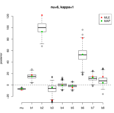
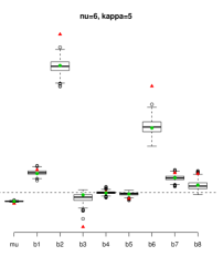
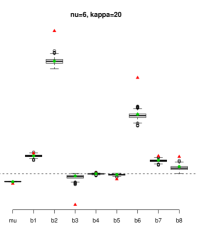
Figure 2: Power-posteriors for the Pima Indian data: $\nu=6$, $\kappa\in\{1,5,20\}$.

Figure 2 summarizes the marginal power posterior(s) for $\beta$ with boxplots. Three settings of $\kappa\in\{1,5,20\}$ (each panel) were used, and heavy regularization (fixing $\nu=6$) was applied. Only the first panel ($\kappa=1$) summarizes samples from the true posterior. The $\kappa>1$ settings are useful for obtaining other estimators. The MLE, obtained from the glm command in R (R Development Core Team,, 2009), and the MAP as estimated from the sample(s), are also shown. Shrinkage is apparent in the divergence between the MAP and MLE values in all panels. Observe how the quartiles and outliers converge on the MAP as $\kappa$ is increased, reflecting higher confidence in the accurate estimation of those values. Convergence is particularly rapid for the intercept term, and the two coefficients with considerable mass near zero ($\beta_{4}$ and $\beta_{5}$). These columns of $X$ have the highest concentration of “missing” values (30% and 49% respectively), so it is not surprising the that MAP estimator excludes them.

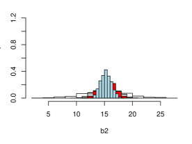
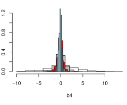
Figure 3: Illustrating the concentration of posterior mass of $\beta_{1}$ and $\beta_{4}$ on the Pima Indian data for $\kappa\in\{1,5,10,20\}$

Figure 3 illustrates how mass concentrates on the MAP in two disparate cases for varying values of $\kappa$. For $\beta_{2}$ (left panel), which is decidedly non-zero in the power posterior(s), the convergence to the MAP (apparently around $\beta_{2}=6$) is modest. In the case of $\beta_{4}$ (right panel) the convergence to the MAP (to zero) is more rapid as $\kappa$ is increased, allowing for confident variable de-selection in a way similar to the lasso for linear regression.

Finally, we consider the case where $\nu$ is also inferred by MCMC, jointly with the other parameters in the model. We use the IG prior on $\nu$ with $(r=2,d=0.1)$, a typical default choice for linear regression (e.g., Gramacy and Pantaleo,, 2010).

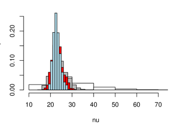
Figure 4: Concentration of posterior mass of $\nu$ on the Pima Indian data for $\kappa\in\{1,5,10,20\}$. The histogram extends to $\nu=100$ when $\kappa=1$, but the figure is trimmed.

Figure 4 shows the marginal posterior for $\nu$ under our settings of $\kappa$. The rate of convergence is modest, with the spread of samples in the $\kappa=20$ case being only half that of the $\kappa=1$ case.

4.2 Comparing c/pdf representations on binomial data

To illustrate the efficient handling of binomial data and, simultaneously, to compare the cdf and pdf representations, consider the following simple binomial logistic regression problem. The true linear predictor is $\eta_{i}=1+x_{i}^{\top}\beta$ where $\beta=(2,-3,2,-4,0,0,0,0,0)^{\top}$, and the $p=9$ dimensional $x_{i}$ are uniform in $[0,1]^{p}$. The responses, $y_{i}\in\{0,\dots,n_{i}\}$, are sampled with $y_{i}|x_{i}\sim\mathrm{Bin}(n_{i},\mu_{i})$ where $n_{i}=20$ and $\mu_{i}=e^{\eta_{i}}/(1+e^{\eta_{i}})$.

	RMSE (sd)
	flat		multi
cdf	0.2117	(0.0602)	0.2120	(0.0606)
pdf	0.2119	(0.0613)	0.2121	(0.0602)

	time (sd)
	flat		multi
cdf	570.4	(37.8)	64.6	(0.82)
pdf	570.2	(28.7)	64.4	(0.99)

Table 1: Comparing RMSEs (left) and timings in seconds (right) of c/pdf representations and flattened/multiplicity treatments of binomial regression modeling.

Table 1 compares four different implementations of regularized binomial logistic regression ($\alpha=1$) based on the output of 100 repeated experiments with $\sum n_{i}=2000$ (i.e., $m=100$ distinct $x_{i}$ predictors). The metrics for comparison are root mean squared error (RMSE) between the true and posterior mean $\beta$s, and overall computing time of the respective MCMC samplers. In all cases, we use $T=1000$ MCMC rounds with MH sampling of $\lambda_{i}$ at thinning level(s) set by $\kappa^{\prime}$ (i.e., via $\kappa^{\prime}_{i}$ for each $\lambda_{i}$) as described in Section 3.1. The first 100 rounds were discarded as burn-in. The left table shows that there is no significant difference between the cdf and pdf representations, or between the flattened or multiplicity handling of binomial data, in terms of RMSE. The right table portrays a more interesting story in terms of CPU times. The many fewer latent variables needed by the multiplicity implementation leads to a much (9x) faster execution compared to flattening, with no cost in accuracy (via RMSE). In contrast, there is no speed gain to using $n$ fewer latent $z_{i}$ variables in the pdf representation.

Figure 5: Comparing MH (left) and slice (right) samplers for a $\lambda_{i}$ in the pdf representation.

Figure 5 illuminates the differences in behavior between the MH and slice sampler for the $\lambda_{i}$ draws (in the pdf representation). A particularly “sticky” case, as chosen from output of the experiment, had $\kappa^{\prime}_{i}=14$. The top panel shows that many proposals from $q_{a,b}$ can be rejected under the MH ratio, even when the chain is automatically thinned. The bottom panel shows the chain obtained for the same $\lambda_{i}$ under the slice sampler, which never saves any rejected draws. However, this comes at the expense of many rejections in the inner–loop of the slice, resulting in a slow overall sampler. The median was four, but the mean was 81 owing to a heavy right-hand tail in the distribution of rejections whose central 95% quantile spanned to 114 and maximum reached 140,600. The overall MCMC scheme based on the slice sampler took four times longer than the one based on MH. Despite the absence of rejections, the mixing in slice sampler chain (assessed visually) was no better than MH. Indeed, their effective sample size due to autocorrelation (Kass et al.,, 1998) was nearly identical: 223 for slice sampling, and 221 for MH. Therefore, MH is recommended for speed considerations.

4.3 A simulated $p\gg n$ experiment

We turn now to a predictive comparison of the methods of this paper, both fully Bayesian and full/joint MAP (including $\nu$), benchmarked against other modern approaches to regularized logistic regression. Consider a synthetic data experiment like the one in Section 4.2 except: $n_{i}=5$ for each of 20 unique predictors $x_{i}$, so that $\sum n_{i}=100$. Three variations on the data-generating $\beta$ vectors were used. In the first case $p=9$ and $\beta=(2,-3,0.74,-0.9,0,0,0,0)^{\top}$; in the second case $p=100$, augmenting $\beta$ from the first case with 91 more zeros; and in the third $p=1000$ with 900 more zeros still. Each experiment involves a new random training design in the unit $p$-cube. Random testing set are created similarly, except that $n_{i}^{\prime}=100$ so $\sum n_{i}^{\prime}=10000$. The metrics of comparison are (approximated) expected log likelihood (ELL) and misclassification rates.

Fully Bayesian posterior mean estimators (i.e., $\kappa=1$) are derived via priors/MCMC exactly as described in the preceding sections with $(100,1000)$, $(500,1500)$, $(1000,2000)$ burn-in and total MCMC rounds in each of the cases $p=9,100,1000$, respectively. MAP estimators are found by running a $\kappa=10$ chain initialized at $(\beta,\lambda,\nu)$-values from the $\kappa=1$ chain used for the mean estimators, except in the $p=1000$ case where $\nu$ was fixed to its posterior mean for reasons laid out in Section 3.2. Comparators include: the MLE obtained via the glm command in R; a binomial fit from the glmnet package (Friedman et al.,, 2010); and the estimator of Krishnapuram et al., (2005) [“krish” for short]. The MLE was unstable in the $p=100$ & $1000$ cases, so these results were omitted. CV was used to choose the penalty parameter in the $p=9$ & $100$ cases for glmnet, via cv.glmnet. The same procedure gave fatal errors in the $p=1000$ case so we plugged in the estimate obtained from the corresponding $p=100$ run in for this final case. Reliably setting the penalty parameter for “krish”, via CV or otherwise, was too computationally intensive for the $p=100,1000$ cases so we picked a setting by hand using out-of-sample simulations from the $p=9$ case.

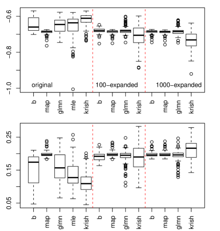
ELL	5%	avg	95%
b	-0.694	-0.646	-0.582
map	-0.710	-0.688	-0.677
glmn	-0.703	-0.650	-0.593
mle	-0.797	-0.658	-0.588
krish	-0.699	-0.619	-0.579
b	-0.701	-0.680	-0.660
map	-0.712	-0.687	-0.678
glmn	-0.705	-0.678	-0.629
krish	-0.815	-0.711	-0.628
b	-0.707	-0.687	-0.676
map	-0.711	-0.689	-0.677
glmn	-0.707	-0.683	-0.639
krish	-0.707	-0.734	-0.651

miss	5%	avg	95%
b	0.065	0.152	0.201
map	0.189	0.199	0.212
glmn	0.092	0.159	0.217
mle	0.074	0.136	0.213
krish	0.061	0.113	0.184
b	0.172	0.191	0.210
map	0.188	0.199	0.212
glmn	0.133	0.189	0.212
krish	0.129	0.189	0.244
b	0.187	0.198	0.215
map	0.188	0.198	0.215
glmn	0.142	0.193	0.214
krish	0.151	0.211	0.252

Figure 6: Expected log likelihood (ELL) and misclassification rates in boxplot (left) and tabular (right) form. In both cases there are three sections, depending on the number of irrelevant predictors in the design matrix, wherein the same estimators are applied. The vertical dashed-red lines in the boxplots indicate the same demarkation as the horizontal lines in the tables.

The results of the Monte Carlo experiment are summarized in Figure 6 by boxplots, and numerically. The best estimators have high ELL, low miss rates, and lower variability across the 100 repetitions. The fully Bayesian and “krish” methods are the best when $p=9$ (left-hand region of the boxplots and the top region of the tables). The former wins by ELL, having fewer low values, and the latter wins on miss rate, having more small ones. The “krish” method wins by both metrics on average, since it employs a fortuitously hand-chosen setting of the penalty parameter. The MLE is good on average, but has some extreme ELL and miss rate values. The glmnet and MAP estimators are positioned in between.

Distinctions in performance between the methods increases with $p$. See the right-hand regions of the boxplots and the bottom regions of the tables. The “krish” method suffers from high variability due to the fixed choice of the penalty parameter. The glmnet variability is much lower, but there are many extreme outliers. Behavior in both $p=100$ and $1000$ cases is qualitatively similar for this estimator even though the former used CV to set the penalty parameter and the latter used the same fixed value. The MAP and fully Bayesian estimators have similar average behavior compared to other estimators, but with lower variability. Apparently, choosing the penalty parameter via the posterior offers the most stability in high dimensional settings. The fully Bayesian approach appears preferable to the MAP in all cases, but this distinction is harder to make out as $p$ increases.

4.4 Spam data with interactions

For a similar real-data experiment, consider the Spambase data set from UCI. It contains the binary classifications of 4601 emails based on 57 attributes which are treated as predictors. An interaction-expanded version of the predictor set contains approximately 1700 predictors. We performed a Monte Carlo experiment comprising of 20 random 5-fold CV training and testing sets using both the original and expanded predictors. Estimators were fit on the 100 training sets, and validated by misclassification rate on the testing ones. The Bayes estimators used (500,1500) MCMC (burn-in, total) rounds with the original 57 attributes, and (1000,2000) with the expanded set. The MAP and glmnet calculations were exactly as described for the $p=100$ case in Section 4.3 for the original predictor set, and like the $p=1000$ case for the expanded one. And “krish” was like $p=9$ and $p=100$, respectively.

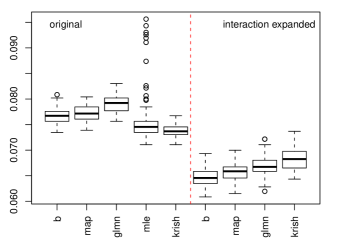
miss	5%	avg	95%
b	0.074	0.077	0.079
map	0.074	0.077	0.080
glmn	0.077	0.079	0.082
mle	0.071	0.076	0.092
krish	0.072	0.074	0.076
b	0.062	0.065	0.068
map	0.063	0.066	0.068
glmn	0.064	0.067	0.070
krish	0.065	0.068	0.072

Figure 7: Misclassification rates in boxplot (left) and tabular (right) form. In both cases there are two sections, depending absence or presence of interaction terms in the design matrix, wherein the same estimators are applied. The vertical dashed-red line in the boxplot indicates the same demarkation as the horizontal line in the table.

The results of the experiment are summarized in Figure 7. The first thing we notice is that, in contrast with the results in Section 4.3, the performance improves as the predictor set expands since some of the interaction terms make good predictors. The MLE is unstable, and so the regularized estimators offer an improvement even when the number of predictors is small relative to the number of instances. The Bayesian methods unilaterally outperform glmnet, and using the posterior to set the value of the regularization parameter is important in high dimensional settings. The “krish” estimator with fortuitous regularization is the best on the original predictor set, but worst on the expanded one where a revised setting of regularization could not be automated efficiently.

5 Discussion and extension

We provide a simulation-based approach to regularized logistic regression that facilitates a variety of inferential goals under a single framework. Most of the development of the methodology, and all of the applications, involved the $\alpha=1$ case. Everything extends to the ridge prior ($\alpha=2$), i.e., an independent normal prior for each coefficient $\beta_{j}$ with variance $\sigma_{j}^{2}\nu^{2}/\kappa$. Then, $p_{\kappa}(\omega_{j}|\beta,\nu)$ is a point mass at $\omega_{j}=1$. Thus similar conjugacy results hold for the gamma prior on $\nu$ and $\nu^{2}$.

From a computational perspective, our methods are competitive with the state-of-the art in un-regularized (and $\kappa=1$) contexts too. For example, we compared the efficiency of our methods to the “dRUM” MH sampler described by Frühwirth-Schnatter and Frühwirth, (2010). This method is attractive because it is fast and easy to implement. For example, on the Pima data it takes about 32s to generate 10,000 samples from the posterior which is about 7x faster than our pdf representation, which took 230s. However, the MH acceptance rate of the dRUM method was 46% which lead to an marginal ESS of 957 averaged over the nine $\beta_{j}$ coefficients. Our pdf representation had an average ESS that was about 5x better, at 4518. So the methods work out to have similar overall efficiences in that example. But in higher dimension like the 57-d spam data, our Gibbs sampling approach is much more attractive. The acceptance rate for dRUM was extremely low at 0.4%, which leads to ESSs that are essentially nil. Although our pdf representation is (again) 7x slower, faster convergence due to better movement in the chain leads to reasonable ESSs around 500.

There are several extensions of our methodology that readily present themselves. For example, handling polychotomous data (i.e., $>2$ classes) is straightforward. Following the setup in HH we may introduce $C$ collections of coefficients $\beta^{(1)},\dots,\beta^{(C)}$ for $C$ classes with the convention that $\beta^{(C)}=0$ so that logistic regression is recovered in the $C=2$ case. Then, we simply work with the conditional likelihoods $L(\beta^{(j)}|y,\beta^{(-j)})$ which turn out to have exactly the form of a logistic regression likelihood for the class indicator that each $y_{i}=j$, independently for $i=1,\dots,n$. If there are $n_{i}>1$ trials for predictors $x_{i}$, then our algorithm for binomial logistic regression is applicable via a vectorized multiplicity parameter as described in Section 3.3. Extending the methods to ordinal responses is even easier. Johnson and Albert, (1999, Chapter 4) describe a Bayesian probit model which may be adapted for the logit case following either HH or our cdf representation. The pdf representation may not be readily applicable because the latent $z_{i}$ are useful for efficient sampling of the ordinal break points.

An further direction is to other classes of regularization priors. Implementing the Normal–Gamma extension (Griffin and Brown,, 2010) requires adding an extra (conjugate) parameter. A promising new approach is the horseshoe prior (Carvalho et al.,, 2010), which can be implemented with the addition of a slice sampler. Often variable selection is a primary goal of regularization, for which our methods would require further extension. For example, HH describe an approach to variable selection for logistic regression via Reversible Jump MCMC (Green,, 1995) which is adaptable to our framework. A similar regularized approach in a linear regression is provided byGramacy and Pantaleo, (2010). For variable selection for logistic regression using spike-and-slab priors, see Tüchler, (2008).

Acknowledgments

This research was partially funded by EPSRC grant EP/D065704/1 to RBG. The authors would like thank Matt Taddy for interesting discussions on the efficient handling of Binomial data, extensions to Multinomial regression, and EM code for the MAP estimator(s). We are grateful to two referees and an associate editor for valuable comments.

Appendix A Posterior conditional for $\beta$ in the pdf representation

For a particular $\lambda$, i.e., ignoring the integral in Eq. (13), we have the following expression for the likelihood in vector/matrix form.

$$\prod_{i=1}^{n}\left(1+e^{-y_{i}x_{i}^{\top}\beta}\right)=e^{ay^{\top}X\beta}\exp\left\{-\frac{1}{2}\left((y.X)\beta+\frac{1}{2}(a-b)\lambda\right)^{\top}\!\Lambda^{-1}\left((y.X)\beta+\frac{1}{2}(a-b)\lambda\right)\right\}$$

An expression for the posterior conditional for $\beta$ can then obtained by multiplying by the kernel of the MVN prior given $\omega$, provided below Eq. (15), namely: $\exp\{-\frac{1}{2}\beta^{\top}\!(\frac{\kappa^{2}}{\nu^{2}}\Sigma^{-1}\Omega^{-1}\beta)\}$. Combining the terms in the three exponents gives the following quadratic form.

$$-\frac{1}{2}\left[-2ay^{\top}X\beta+\!\left((y.X)\beta+\frac{1}{2}(a-b)\lambda\right)^{\!\top}\!\!\!\Lambda^{-1}\!\left((y.X)\beta+\frac{1}{2}(a-b)\lambda\right)\!+\beta^{\top}\!\left(\frac{\kappa^{2}}{\mu^{2}}\Sigma^{-1}\Omega^{-1}\!\right)\!\beta\right]$$

Collecting terms for $\beta$ yields

$$\beta^{\top}\left((y.X)^{\top}\Lambda^{-1}(y.X)+\frac{\kappa^{2}}{\nu^{2}}\Sigma^{-1}\Omega^{-1}\right)\beta-(2ay^{\top}X-(a-b)(y.X)\Lambda^{-1}\lambda)\beta.$$

Therefore we deduce that the conditional is $\mathcal{N}_{p}(\tilde{\beta},V)$ where $V^{-1}=(y.X)^{\top}\Lambda^{-1}(y.X)+\frac{\kappa^{2}}{\nu^{2}}\Sigma^{-1}\Omega^{-1}$. Recognizing that $(y.X)\Lambda^{-1}\lambda=X^{\top}y$ gives that $\tilde{\beta}=V(a-\frac{1}{2}[a-b])X^{\top}y$.

Appendix B Generalized Inverse Gaussian distribution

The pdf of a Generalized Inverse Gaussian, $\mathrm{GIG}(\lambda,\chi,\psi)$ is

$$g(x;\lambda,\chi,\psi)=\frac{(\psi/\chi)^{\lambda/2}}{2K_{\lambda}(\sqrt{\psi\chi})}x^{\lambda-1}\exp\left\{-\frac{1}{2}(\psi x+\chi/x)\right\},$$

where $K_{\lambda}$ is a modified Bessel function of the second kind. If $X\sim\mathrm{GIG}\!\left(\frac{1}{2},\chi,\psi\right)$ then $X^{-1}\sim\mathrm{IN}(\mu=\sqrt{\psi/\chi},\lambda=\psi)$ where where $\mathrm{IN}$ is the inverse Gaussian distribution with pdf

$$f(x;\mu,\lambda)=\sqrt{\frac{\lambda}{2\pi x^{3}}}\exp\left\{-\frac{\lambda\left(x-\mu\right)^{2}}{2\mu^{2}x}\right\}.$$

The mean and variance are $\mathbb{E}\{x\}=\mu$ and $\mathrm{\mathbb{V}ar}[x]=\mu^{3}/\lambda$. A generalized inverse Gaussian $\mathrm{GIG}\left(\frac{1}{2},\chi,\psi\right)$ is an inverse of an Inverse Gaussian. For simulation from $\mathrm{GIG}$ and $\mathrm{IN}$ distributions see Devroye, (1986).

References

- Andrews and Mallows, (1974) Andrews, D. and Mallows, C. (1974). “Scale Mixtures of Normal Distributions.” Journal of the Royal Statistical Soceity, Series B, 36, 99–102.
- Asuncion and Newman, (2007) Asuncion, A. and Newman, D. (2007). “UCI Machine Learning Repository.”
- Barndorff-Nielsen et al., (1982) Barndorff-Nielsen, O., Kent, J., and Sorensen, M. (1982). “Normal Variance-Mean Mixtures and -distributions.” International Statistical Review, 50, 145–159.
- Bernstein, (2005) Bernstein, D. (2005). Matrix Mathematics. Princeton, NJ: Princeton University Press.
- Box and Tiao, (1973) Box, G. and Tiao, G. (1973). Bayesian Inference in Statistical Analysis. Mass: Addison Wesley.
- Carlin and Polson, (1991) Carlin, B. P. and Polson, N. G. (1991). “Inference for Nonconjugate Bayesian Models using the Gibbs sampler.” The Canadian Journal of Statistics, 19, 4, 399–405.
- Carvalho et al., (2010) Carvalho, C., Polson, N., and Scott, J. (2010). “The horseshoe estimator for sparse signals.” Biometrika, 9, 2, 465–480.
- Devroye, (1986) Devroye, L. (1986). Non-Uniform Random Variate Generation. Springer-Verlag.
- Doucet et al., (2002) Doucet, A., Godsill, S., and Robert, C. (2002). “Marginal maximum a posteriori estimation using Markov chain Monte Carlo.” Statistics and Computing, 21, 77–84.
- Fahrmeir et al., (2010) Fahrmeir, L., Kneib, T., and Konrath, S. (2010). “Bayesian regularisation in structured additive regression: A unifying perspective on shrinkage, smoothing and predictor selection.” Statistics and Computing, 203–219.
- Friedman et al., (2010) Friedman, J. H., Hastie, T., and Tibshirani, R. (2010). “Regularization Paths for Generalized Linear Models via Coordinate Descent.” Journal of Statistical Software, 33, 1, 1–22.
- Friel and Pettitt, (2008) Friel, N. and Pettitt, A. (2008). “Marginal likelihood estimation via power posteriors.” Journal of the Royal Statistical Society, Series B., 70, 3, 589–607.
- Frühwirth-Schnatter and Frühwirth, (2007) Frühwirth-Schnatter, S. and Frühwirth, R. (2007). “Auxilliary Mixture Sampling with Applications to Logistic Models.” Computational Statistics and Data Analysis, 51, 7, 3509–3528.
- Frühwirth-Schnatter and Frühwirth, (2010) — (2010). “Data augmentation and MCMC for binary and multinomial logit models.” In Statistical Modelling and Regression Structures – Festschrift in Honour of Ludwig Fahrmeir, eds. T. Kneib and G. Tutz, 111–132. Physica-Verlag.
- Frühwirth-Schnatter et al., (2009) Frühwirth-Schnatter, S., R., Frühwirth, Held, L., and Rue, H. (2009). “Improved auxiliary mixture sampling for hierarchical models of non-Gaussian data.” Statistics and Computing, 19, 479–492.
- Genkin et al., (2007) Genkin, A., Lewis, D., and Madigan, D. (2007). “Large-Scale Bayesian Logistic Regression for Text Categorization.” Technometrics, 49, 3, 291–304.
- Godsill, (2000) Godsill, S. (2000). “Inference in symmetric alpha-stable noise using MCMC and the slice sampler.” In IEEE International Conference on Acoustics, Speech and Signal Processing, vol. VI, 3806–3809.
- Gramacy and Pantaleo, (2010) Gramacy, R. and Pantaleo, E. (2010). “Shrinkage regression for multivariate inference with missing data, and an application to portfolio balancing.” Bayesian Analysis, 5, 2, 237–262.
- Green, (1995) Green, P. (1995). “Reversible Jump Markov Chain Monte Carlo Computation and Bayesian Model Determination.” Biometrika, 82, 711–732.
- Griffin and Brown, (2010) Griffin, J. E. and Brown, P. J. (2010). “Inference with Normal–Gamma prior distributions in regression problems.” Bayesian Analysis, 5, 1, 171–188.
- Hans, (2009) Hans, C. (2009). “Bayesian Lasso Regression.” Biometrika, 96, 836–845.
- Holmes and Held, (2006) Holmes, C. and Held, K. (2006). “Bayesian Auxilliary Variable Models for Binary and Multinomial Regression.” Bayesian Analysis, 1, 1, 145–168.
- Jacquier et al., (2007) Jacquier, E., Johannes, M., and Polson, N. (2007). “MCMC Maximum Likelihood for Latent State Models.” Journal of Econometrics, 137, 615–640.
- Johnson and Albert, (1999) Johnson, V. and Albert, J. (1999). Ordinal Data Modeling. Springer-Verlag.
- Kass et al., (1998) Kass, R. E., Carlin, B. P., Gelman, A., and Neal, R. M. (1998). “Markov Chain Monte Carlo in Practice: A Roundtable Discussion.” The American Statistician, 52, 2, 93–100.
- Kirkpatrick et al., (1983) Kirkpatrick, S., Gelatt, C., and Vecci, M. (1983). “Optimization by simulated annealing.” Science, 220, 671–680.
- Krishnapuram et al., (2005) Krishnapuram, B., Carin, L., Figueiredo, M., and Hartemink, A. (2005). “Sparse Multinomial Logistic Regression: Fast Algorithms and Generalization Bounds.” IEEE Pattern Analysis and Machine Intellegence, 27, 6, 957–969.
- Madigan and Ridgeway, (2004) Madigan, D. and Ridgeway, G. (2004). “Discussion of ‘Least Angle Regression’ by B. Efron, T. Hastie, I. Johnstone, and R. Tibshirani.” Annals of Statistics, 32, 2, 465–469.
- Park and Hastie, (2008) Park, M. and Hastie, T. (2008). “Penalized Logistic Regression for Detecting Gene Interactions.” Biostatistics, 9, 1, 30–50.
- Park and Casella, (2008) Park, T. and Casella, G. (2008). “The Bayesian Lasso.” Journal of the American Statistical Association, 103, 482, 681–686.
- Pincus, (1968) Pincus, M. (1968). “A Closed Form Solution of Certain Programming Problems.” Operations Research, 18, 1225–1228.
- Robert, (1995) Robert, C. (1995). “Simulation of Truncated Normal Variables.” Statistics and Computing, 5, 2, 121–125.
- R Development Core Team, (2009) R Development Core Team (2009). R: A Language and Environment for Statistical Computing. R Foundation for Statistical Computing, Vienna, Austria. ISBN 3-900051-07-0.
- Tibshirani, (1996) Tibshirani, R. (1996). “Regression shrinkage and Selection via the Lasso.” Journal of the Royal Statistical Society, Series B., 58, 1, 267–288.
- Tüchler, (2008) Tüchler, R. (2008). “Bayesian variable selection for logistic models using auxiliary mixture sampling.” Journal of Computational and Graphical Statistics, 17, 76–94.
- Weron, (1996) Weron, R. (1996). “On the Chambers-Mallows-Stuck Method for Simulating Skewed Stable Random Variables.” Statistics and Probability Letters, 28, 2, 165–171.
- West, (1987) West, M. (1987). “On Scale Mixtures of Normal Distributions.” Biometrika, 74, 3, 646–648.