Effective swimming strategies in low Reynolds number flows

Abstract

The optimal strategy for a microscopic swimmer to migrate across a linear shear flow is discussed. The two cases, in which the swimmer is located at large distance, and in the proximity of a solid wall, are taken into account. It is shown that migration can be achieved by means of a combination of sailing through the flow and swimming, where the swimming strokes are induced by the external flow without need of internal energy sources or external drives. The structural dynamics required for the swimmer to move in the desired direction is discussed and two simple models, based respectively on the presence of an elastic structure, and on an orientation dependent friction, to control the deformations induced by the external flow, are analyzed. In all cases, the deformation sequence is a generalization of the tank-treading motion regimes observed in vesicles in shear flows. Analytic expressions for the migration velocity as a function of the deformation pattern and amplitude are provided. The effects of thermal fluctuations on propulsion have been discussed and the possibility that noise be exploited to overcome the limitations imposed on the microswimmer by the scallop theorem have been discussed.

1 Introduction

There has been recently a resurgence of interest in low Reynolds number swimming. Particular attention has been given to discrete designs purcell77 ; najafi04 ; avron05 , which allow simpler description of the geometrical aspects of the problem, and identification of the necessary ingredients for propulsion.

One of the reasons for renewed interest is the progress in mechanical manipulation at the microscale, which has allowed the realization of the first examples of artificial microscopic swimmers dreyfus05 ; yu06 ; behkam06 ; leoni09 . These examples constitute the first step towards the construction of ”microbots”, whose application would be wide-spread, e.g. in medicine, as microscopic drug carriers in not otherwise accessible regions of the human body. At the present stage, however, most of such artificial swimmers are driven by external fields, and the problem of an autonomous power source remains under study.

Several solutions to this problem have been proposed. Among them, various methods of rectification of Brownian motion lobaskin08 ; golestanian09 , and mechanical reactions in the swimmer body, induced by inhomogeneity in the environment, e.g. presence of a chemical gradient golestanian05 ; paxton06 ; pooley07 .

It has recently been suggested, that a microswimmer may extract the energy needed for locomotion, out of the velocity gradients in an external flow olla10 . Based on a discrete design, that is a generalization of the three-bead swimmer of najafi04 ; earl07 ; golestanian08 , it was shown that a microswimmer could migrate across a linear shear flow, by a sequence of deformations induced by the external flow itself. A continuous version of this microswimmer has been described in olla10a , based on the analogy of the deformation sequence in the discrete case, with the tank-treading motion regime of a vesicle (or of a microcapsule) in a linear shear flow keller82 ; kraus96 ; barthes80 .

Through tank-treading, a microscopic object such as a vesicle, is able to maintain a fixed shape and orientation in an external flow, with its surface circulating around its interior, precisely as a tank-tread note . The existence of a preferential shape and orientation for the object, turns out to be one of the main ingredients for migration in an external flow. It should be mentioned that tank-treading has already a long history, as a propulsion candidate for swimming in quiescent fluids purcell77 ; leshansky08 . Other examples of migration induced by simultaneous rotation and deformation of solid objects in viscous shear flows, have been analyzed both theoretically watari09 and experimentally marcos09 . The design of a microswimmer that uses its internal degrees of freedom to spin rather than to swim, has been proposed in dreyfus05a .

The interesting aspect of external flow aided propulsion, is that the migration velocity scales linearly in the stroke amplitude. This behavior is not surprising: the migration velocity of tank-treading vesicles in wall bounded flows, scales linearly with the deviation from spherical shape olla97 ; abkarian02 ; olla00 ; danker09 . In contrast, the velocity of a microswimmer in a quiescent fluid, due to the constrains imposed by the scallop theorem purcell77 , is characterized by quadratic scaling shapere89 .

In the present paper, the analysis in olla10 , which focused on the behavior of a discrete microswimmer in an infinite domain, will be extended to the case of a wall bounded flow. Particular attention will be given to identification of the deformation patterns associated with migration in different flow conditions, and with energy extraction from the flow. A simple semi-quantitative analysis of the effect of thermal fluctuations will be provided as well, along the lines of the approach described in dunkel09 .

The generation of specific deformation patterns, requires the presence of a control system, modulating the response of the microswimmer to the external flow (after all, this is what characterizes a microswimmer, as compares to, say, a simple vesicle). The possibility of control through modification of the swimmer structural properties will therefore be examined, and a simple example of control, by braking on the swimmer moving parts, will be described in detail.

The paper is organized as follows. In Sec. 2, the basic equations of the model are presented and in Sec. 3, the results in olla10 are briefly summarized. In Sec. 4, the analysis is extended to the case of a wall bounded flow. In Sec. 5, the mechanism of energy extraction from the flow is discussed. The structural dynamics of the swimmer is discussed in Sec. 6. In Sec. 7 an hypothesis of control system to achieve migration is discussed. In Sec. 8, the effect of thermal noise on passive swimming is analyzed. Section 9 is devoted to conclusions. Technical details on the swimmer behavior in a wall bounded flow are provided in the Appendix.

2 Swimming strategy in free space

We analyze the behavior of the simple swimmer depicted in Fig. 1. Contrary to najafi04 ; golestanian08 , who considered a linear device, the three beads in the swimmer under study are located, at rest, at the vertices of an equilateral triangle of side $R$.

Figure 1: Rest configuration of the three-bead swimmer. Small case indicates the reference frame rotating solidly with the device.

The swimmer is placed in in a linear shear flow

$$\bar{\bf U}({\bf X})=\bar{\bf U}(0)+(0,\alpha X_{1},0),$$ (1)

and wants to migrate along the gradient direction $X_{1}$.

We are interested in a situation in which the system is able to move by internal deformation without the aid of external forces. We assume the links between the beads in the trimer to be immaterial and the bead radii $a$ to be much smaller than $R$. Including terms up to $O(a/R)$, the equation of motion for the device can be written in the form:

$$\dot{\bf X}_{i}=\bar{\bf U}({\bf X}_{i})+\tilde{\bf U}_{i}(t)+{\bf F}_{i}(t)/\sigma,$$ (2)

where ${\bf X}_{i}$ is the coordinate of the $i$-th bead, ${\bf F}_{i}(t)$ is the force on bead $i$ by the rest of the trimer, $\sigma=6\pi\mu a$, with $\mu$ the fluid viscosity, is the Stokes drag, and $\tilde{\bf U}_{i}(t)$ is the flow perturbation in ${\bf X}_{i}$ generated by the other beads in the trimer.

To lowest order in $a/R$, the flow perturbation is obtained replacing the beads by point forces in the fluid, with intensity equal to the Stokes drag exerted by the beads (stokeslet approximation happel ):

$$\tilde{\bf U}_{i}(t) = \sum_{j\neq i}{\boldsymbol{\sf T}}({\bf X}_{i}-{\bf X}_{j}){\bf F}_{j};$$ (3)

$${\boldsymbol{\sf T}}({\bf X}) = \frac{3a}{4\sigma}\Big{[}\frac{{\bf 1}}{|{\bf X}|}+\frac{{\bf X}{\bf X}}{|{\bf X}|^{3}}\Big{]},$$ (4)

where ${\boldsymbol{\sf T}}({\bf X}_{i}-{\bf X}_{j})$, for $i\neq j$, is the off-diagonal part of the so called Oseen tensor happel .

Linearity of the shear, Eq. (1), and absence of external forces, $\sum_{i}{\bf F}_{i}=0$, imply that the trimer center of mass ${\bf X}^{\scriptscriptstyle{\rm CM}}=({\bf X}_{1}+{\bf X}_{2}+{\bf X}_{3})/3$ would move, if one disregarded the flow perturbation, as a point tracer at ${\bf X}^{\scriptscriptstyle{\rm CM}}$: $\dot{\bf X}^{\scriptscriptstyle{\rm CM}}=\bar{\bf U}({\bf X}^{\scriptscriptstyle{\rm CM}})+(1/3)\sum_{i}{\bf U}_{i}(t)$. Time averaging the deviation with respect to $\bar{\bf U}({\bf X}^{\scriptscriptstyle{\rm CM}})$, we obtain the migration velocity

$${\bf U}^{migr}=(1/3)\sum_{i}\langle\tilde{\bf U}_{i}\rangle=\langle\tilde{\bf U}_{1}\rangle.$$ (5)

The velocity perturbation $\tilde{\bf U}_{1}$ is the sum of the stokeslet fields $\tilde{\bf U}({\bf X}|{\bf X}_{i},{\bf F}_{i})$, $i=2,3$ generated in ${\bf X}={\bf X}_{1}$ by beads $2$ and $3$. We assume exchange symmetry among the beads, in the sense that trimer configurations at angles $\phi+2n\pi/3$ are indistinguishable. This mimicks the stationary tank-treading regime of a vesicle, as the trimer arms will extend (or contract) in identical way, when reaching a given position in the laboratory reference frame. Exchange symmetry allows us to rewrite Eq. (5) in the equivalent form: ${\bf U}^{migr}=\langle[\tilde{\bf U}({\bf X}_{2}|{\bf X}_{1},$ ${\bf F}_{1})+\tilde{\bf U}({\bf X}_{3}|{\bf X}_{1},{\bf F}_{1})]\rangle$.

Focusing on the effect of stokeslet 1 on beads 2 and 3, rather than on the one of stokelets 2 and 3 on bead 1, allows to understand geometrically the swimming strategy of the trimer, as illustrated in Fig. 2 (we consider for the moment the case of an unbounded domain).

Figure 2: The swimming strategy: link $23$ is contracted at $\phi=\pi/2$ (top-left) and stretched at $\phi=-\pi/2$ (top-right); this causes beads 2 and 3 to sample the stokeslet field by bead 1 [continuous line; see Eqs. (3-4)] differently in the two configurations. The unbalance between the two configurations, caused by deformation, is responsible for migration. Dashed lines indicate the strain components of $\bar{\bf U}$ producing the stokeslet in the two cases. Bottom figure: decomposition of $\bar{\bf U}({\bf X})$ into strain and vorticity component.

As shown in olla10 [see Eq. (10) below], the undeformed trimer will rotate in the field $\bar{\bf U}({\bf X})$ with constant frequency, equal to the flow vorticity $\alpha/2$. Because of this, to lowest order in the deformation, $\tilde{\bf U}({\bf X}|{\bf X}_{1},{\bf F}_{1})$ will be the stokeslet field generated by action of the strain component of $\bar{\bf U}$ on a (fixed) bead at position ${\bf X}_{1}$. We see that the the $X_{1}$ component of the stokeslet field generated by bead 1 in response to the strain component of $\bar{\bf U}$ is negative or positive depending on whether $0<\phi<\pi$ or $\pi<\phi<2\pi$. Due to the approximately constant rotation frequency, the trimer will spend an equal time at the two orientations indicated in figure, and, in the case of the undeformed trimer, the contributions to $U_{1}^{migr}$ from the two orientations would cancel by symmetry. Deformations, however, break this symmetry and beads 2 and 3 will sample components $\tilde{U}_{1}({\bf X}_{2,3}|{\bf X}_{1},{\bf F}_{1})$ that are in general of different amplitude. The end result is $\langle\tilde{U}_{1}({\bf X}_{2,3}|{\bf X}_{1},{\bf F}_{1})\rangle\neq 0$, which leads to migration along $X_{1}$.

Quantitative analysis [see Eq. (14) below] shows that the deformation sequence illustrated in Fig. 2 will lead to migration of the trimer to positive $X_{1}$ (to the right in figure).

We notice at this point that migration would be achieved also if just one arm in the trimer performed the stretching-contraction sequence in Fig. 2. [For small deformations, it is possible to see that the migration velocity would just be reduced by $1/3$ with respect to Eq. (5)]. We thus see that the presence of an external flow makes one degree of freedom sufficient for locomotion. We recall that the scallop theorem would prevent this, in the case of a microswimmer in a quiescent fluid purcell77 . Similar “violations” of the scallop theorem were observed in alexander08 ; lauga08 , in which case, the role of the external flow was played by the perturbation generated in the fluid by other swimmers. We shall see in Sec. 8, how a similar result could be obtained exploiting the presence of thermal fluctuations.

3 Migration in free space; quantitative theory

To analyze the deformation dynamics of the trimer, it is convenient to work in the rotating reference; Small case will identify vectors measured in the rotating reference frame (see Fig. 1). In the absence of rotational diffusion, the motion of the trimer will be the sum of a translation and a rotation in the plane $X_{2}X_{3}$, with rotation frequency $\Omega=\dot{\phi}$, where $\phi$, as indicated in Fig. 1, is the angle between the two reference frames.

We are interested in a regime of small deformations, and will proceed perturbatively in the deformation amplitude. In particular, we will have, for the bead position in the rotating frame: ${\bf x}_{i}={\bf x}_{i}^{\scriptscriptstyle{(0)}}+\tilde{\bf x}_{i}$, with ${\bf x}_{i}^{\scriptscriptstyle{(0)}}$ giving the bead positions for the undeformed trimer: ${\bf x}^{\scriptscriptstyle{(0)}}_{1}/R=(1/\sqrt{3},$ $0,0)$, ${\bf x}_{2}^{\scriptscriptstyle{(0)}}/R=-(1/(2\sqrt{3}),1/2,0)$, ${\bf x}_{3}^{\scriptscriptstyle{(0)}}/R$ $=(-1$ $/(2\sqrt{3}),1/2,0)$, and $\tilde{\bf x}_{i}$ accounting for the deformations. We can express the trimer deformations in terms of three arbitrary independent parameters $z_{i}$ (that with two translational and one rotational degrees of freedom make up the six-dimensional configuration space of the trimer in the plane $X_{1}X_{2}$). With the choice

$$\tilde{\bf x}_{1} = \frac{R}{2}\Big{(}\sqrt{3}(z_{2}+z_{3}),z^{\scriptscriptstyle{(n)}}_{3}-z_{2},0\Big{)},$$

$$\tilde{\bf x}_{2} = \frac{R}{2}\Big{(}-\sqrt{3}z_{3},-2z_{1}-z_{3},0\Big{)},$$ (6)

$$\tilde{\bf x}_{3} = \frac{R}{2}\Big{(}-\sqrt{3}z_{2},2z_{1}+z_{2},0\Big{)},$$

the deformation corresponding to just one $z_{i}$ being non-zero, will describe stretching/contraction of the link opposite to bead $i$, while bead $i$ remains fixed in the plane $x_{1}x_{2}$ (see Fig. 3).

Figure 3: Deformations of the trimer corresponding to $z_{i}>0$ for $i=1,2,3$. In the three cases $z_{j}=0$ for $j\neq i$.

Assuming a stationary dynamics for the trimer, with exchange symmetry between the beads, we can write:

$$z_{i}=\sum_{n}[A_{n}\cos n\phi_{i}+B_{n}\sin n\phi_{i}],$$ (7)

where $\phi_{1}=\phi$, $\phi_{2,3}=\phi\mp 2\pi/3$. It will be expedient in calculating the energy balance for locomotion to consider a hierarchy of deformations of increasing order in some small parameter. We thus write $z_{i}=z_{i}^{\scriptscriptstyle{(1)}}+z_{i}^{\scriptscriptstyle{(2)}}+\ldots$, with the normalized deformation amplitude $z=\langle\sum_{i}(z_{i}^{\scriptscriptstyle{(1)}})^{2}\rangle$ playing the role of expansion parameter for the theory, Superscripts will be used to indicate the order in $z$ at which a quantity is evaluated.

Perturbative analysis of Eq. (2) using Eqs. (1) and (6) gives the result olla10 :

$${\bf f}_{1}^{\scriptscriptstyle{(0)}}=\frac{\alpha\sigma R}{\sqrt{3}}\Big{(}-\frac{1}{2}\sin 2\phi,-\frac{1}{2}\cos 2\phi\Big{)}.$$ (8)

and, to next order

$$f_{11}^{\scriptscriptstyle{(1)}} = \frac{\alpha\sigma R}{2}\Big{\{}\frac{\sqrt{3}}{2}[{z^{\scriptscriptstyle{(1)}}_{2}}^{\prime}+{z^{\scriptscriptstyle{(1)}}_{3}}^{\prime}-(z^{\scriptscriptstyle{(1)}}_{2}+z^{\scriptscriptstyle{(1)}}_{3})$$

$$\times \sin 2\phi]-\frac{1}{2}(z^{\scriptscriptstyle{(1)}}_{3}-z^{\scriptscriptstyle{(1)}}_{2})\cos 2\phi\Big{\}},$$

$$f_{12}^{\scriptscriptstyle{(1)}} = \frac{\alpha\sigma R}{2}\Big{\{}\frac{1}{2}({z^{\scriptscriptstyle{(1)}}_{3}}^{\prime}-{z^{\scriptscriptstyle{(1)}}_{2}}^{\prime})$$ (9)

$$- \frac{1}{\sqrt{3}}(z^{\scriptscriptstyle{(1)}}_{1}+z^{\scriptscriptstyle{(1)}}_{2}+z^{\scriptscriptstyle{(1)}}_{3})\cos 2\phi\Big{\}},$$

where primes indicate derivative with respect to $\phi$. Notice that we have disregarded the contribution from the velocity perturbation $\tilde{\bf U}_{i}$ to the force in Eq. (2). Clearly, ${\bf f}_{1}^{\scriptscriptstyle{(0)}}$ is the reaction force of the rigid trimer against the external flow, and ${\bf f}^{\scriptscriptstyle{(1)}}_{1}$ accounts for deformation. Notice that the only contribution strictly qualifying as swimming is the one proportional to $\dot{\bf x}_{1}^{\scriptscriptstyle{(1)}}$ in ${\bf f}^{\scriptscriptstyle{(1)}}$ [the ${z_{2,3}}^{\prime}$ terms in Eq. (9); see also Eq. (7)], the remnant being better described as “sailing”.

The same analysis leading to Eq. (9) gives for the rotation frequency olla10 :

$$\Omega = \frac{\alpha}{4}\{2+[\sqrt{3}\,(z^{\scriptscriptstyle{(1)}}_{2}-z^{\scriptscriptstyle{(1)}}_{3})\sin 2\phi+(z^{\scriptscriptstyle{(1)}}_{2}$$ (10)

$$+ z^{\scriptscriptstyle{(1)}}_{3}-2z^{\scriptscriptstyle{(1)}}_{1})\cos 2\phi]+O(z^{2})\},$$

and from stationarity of the system, we can replace time averages with angular averages:

$$\langle h\rangle=\frac{1}{\pi\alpha}\int_{0}^{2\pi}\Omega(\phi)h(\phi){\rm d}\phi.$$ (11)

Expanding $\Omega$ in powers of $z$, we can then write the average in the above equation as a sum of contributions of increasing order in $z$: $\langle.\rangle=\langle.\rangle^{\scriptscriptstyle{(0)}}+\langle.\rangle^{\scriptscriptstyle{(1)}}+\ldots$, with $\langle f\rangle^{\scriptscriptstyle{(n)}}=(\pi\alpha)^{-1}\int_{0}^{2\pi}\Omega^{\scriptscriptstyle{(n)}}(\phi)f(\phi){\rm d}\phi$.

Knowledge of the force in the rotating reference frame, allows to write for the migration velocity, substituting Eq. (4) into Eq. (5):

$${\bf U}^{migr}=\langle{\boldsymbol{\sf R}}{\boldsymbol{\sf T}}_{1}{\bf f}_{1}\rangle,$$ (12)

where ${\boldsymbol{\sf T}}_{1}={\boldsymbol{\sf T}}({\bf x}_{2}-{\bf x}_{1})+{\boldsymbol{\sf T}}({\bf x}_{3}-{\bf x}_{1})$ and ${\boldsymbol{\sf R}}$ is the rotation matrix back to the laboratory frame:

$$R_{11}=R_{22}=\cos\phi;\quad R_{21}=-R_{12}=\sin\phi.$$ (13)

A simple calculation, including terms up to $O(z$ $\times a/R)$ gives for the Oseen tensor ${\boldsymbol{\sf T}}_{1}$: $T_{1}^{11}=\beta\{7/2-[13z_{1}+29(z_{2}+z_{3})]/8\}$, $T_{1}^{12}=T_{1}^{21}=\beta(\sqrt{3}/8)(z_{2}-z_{3})$ and $\tilde{T}_{1}^{22}=\beta\{5/2+[2z_{1}-31(z_{2}+z_{3})]/\}8$, with $\beta=3a/(4\sigma R)$. Substitution into Eq. (12) and exploiting Eqs. (8-10), gives the final result, to lowest order in $a/R$ and $z$:

$$U_{1}^{migr}=-\frac{\sqrt{3}\alpha a}{256}\Big{[}73B^{\scriptscriptstyle{(1)}}_{1}+13B^{\scriptscriptstyle{(1)}}_{3}\Big{]};$$ (14)

thus $U^{migr}/(\alpha R)=O(za/R)$. Let us consider the contribution $B_{1}\sin\phi_{1}$. We see from Fig. 2, that the stokeslet field generated by bead 1 in response to the strain component of $\bar{\bf U}$, has a positive or negative component at beads $2,3$, depending on whether $0<\phi<\pi$ or $\pi<\phi<2\pi$. Migration is produced by the deformation induced symmetry breaking between the two orientations.

4 Migration in the presence of a wall

A solid wall bounding the flow provides the swimmer with an additional mechanism for migration. The flow perturbation by the swimmer will be the superposition of what would be produced in free space, and a wall correction that can be expressed as a sum of images and counterimages of the freee-space perturbation, generated alternatively at the wall and at the surface of the beads happel . In the stokeslet approximation of Eqs. (2) and (3-4), only the first image has to be taken into considerations.

The migration mechanism is illustrated in Fig. 4, in the case of an elongated object: the image at the wall of the free-space perturbation, because of the asymmetry of the configuration, has a component at the object center, that pushes it away from the wall.

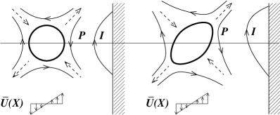
Figure 4: The lift on an elongated object in a wall bounded flow. Dashed arrows indicate the strain component of $\bar{\bf U}({\bf X})$. In the case of a sphere, the flow perturbation $P$ and of the image $I$ are reflection invariant around the plane perpendicular to the flow passing at the sphere center, and the transverse drift is zero. In the case of an elongated object, with the long axis along the stretching direction of the strain, the lobes of the flow perturbation and of the image will be tilted upwards, and the image field at the object position will have a net component to the left. The opposite will occur for an orientation at $\pi/2$ with respect to the one in figure.

Now, a rigid object, with the exception of the very elongated structures described in bretherton62 , will rotate because of the flow vorticity. Because of this, such an object will typically alternate between a condition of outward and inward drift with respect to the wall, and the transverse migration velocity will be zero.

In the case of deformable objects, e.g. vesicles, a fixed orientation and a non-zero transverse drift can be achieved by means of tank-treading keller82 .

In the case of the triangular trimer, tank treading could be mimicked by means of cyclic contraction of its arms: the arms contract when rotation leads them into the contracting (expanding) quadrant of the external strain. This will produce an overall elongated shape oriented along the expanding (contracting) strain direction, and lead to a non-zero transverse migration velocity. To determine the contribution to migration from presence of the wall, it is necessary to determine the image of the stokeslet field of the beads in the trimer.

Let us suppose the wall to be located at coordinate $X_{1}=L$ with respect to the trimer center of mass. Let us denote by $\tilde{\bf U}^{I}({\bf X}|{\bf X}_{i},{\bf F}_{i})$ the image of the stokeslet field $\tilde{\bf U}({\bf X}|{\bf X}_{i},{\bf F}_{i})$ generated in free space by the $i$-th bead. In Eq. (12), we thus have to add a wall contribution:

$$\Delta{\bf U}^{migr}=(1/3)\sum_{ij}\langle\tilde{\bf U}^{I}({\bf X}_{j}|{\bf X}_{i},{\bf F}_{i})\rangle.$$

For small $R/L$, we can Taylor expand $\tilde{\bf U}^{I}({\bf X}_{j}|{\bf X}_{i},$ ${\bf F}_{i})$ around ${\bf X}_{i,j}=0$. From linearity of low Reyn- olds number hydrodynamics, we can write $\tilde{\bf U}^{I}({\bf X}$ $|{\bf X}_{i},{\bf F}_{i})={\boldsymbol{\sf I}}({\bf X}|{\bf X}_{i}){\bf F}_{i}$, with ${\boldsymbol{\sf I}}$ some tensor, and the lowest order contribution in $R/L$ will be ${\boldsymbol{\sf I}}(0|0)\langle\sum_{i}{\bf F}_{i}\rangle=0$. As regards the first order terms, from $\sum_{j}{\bf X}_{j}=0$, we have, identifying the three bead contributions with the one from bead 1: $\langle\sum_{j}{\bf X}_{j}\cdot\nabla\tilde{\bf U}^{I}({\bf X}|0,{\bf F}_{1})\rangle_{{\bf X}=0}=0$. We thus remain with a wall contribution to migration:

$$\Delta{\bf U}^{migr} = 3\langle({\bf X}_{1}\cdot\nabla)\tilde{\bf U}^{I}(0|{\bf X},{\bf F}_{1})\rangle_{{\bf X}=0}$$ (15)

$$+ O((R/L)^{3}),$$

and, from $\tilde{\bf U}^{I}({\bf X}|{\bf X}_{i},{\bf F}_{i})={\boldsymbol{\sf I}}({\bf X}|{\bf X}_{i}){\bf F}_{i}$, we expect a result in the form $\Delta U_{\alpha}^{migr}=H_{\alpha\beta\gamma}\langle X_{1\beta}F_{1\gamma}\rangle$ (summation over repeated vector indices is assumed).

In order to determine the coefficients $H_{\alpha\beta\gamma}$, we must know the image field in Eq. (15). The image field of a stokeslet induced by a solid wall bounding the flow was calculated in blake71 . Its derivation is outlined for reference in the Appendix. We find for the image field derivatives entering Eq. (15):

$$\partial_{X_{1}}\tilde{U}^{I}_{1}(0|{\bf X},{\bf F}_{1})|_{{\bf X}=0} = -\frac{9aF_{11}}{16\sigma L^{2}},$$

$$\partial_{X_{2}}\tilde{U}^{I}_{1}(0|{\bf X},{\bf F}_{1})|_{{\bf X}=0} = \frac{9aF_{12}}{32\sigma L^{2}}.$$ (16)

Substituting into Eq. (15), leads to the result:

$$\Delta U^{migr}_{1}=\frac{27a}{16\sigma L^{2}}\langle M_{\alpha\beta}x_{1\alpha}f_{1\beta}\rangle,$$ (17)

where $M_{\alpha\beta}=(-R_{1\alpha}R_{1\beta}+\frac{1}{2}R_{2\alpha}R_{2\beta})$. From Eq. (13):

$$M_{\alpha\beta}=\begin{pmatrix}-\frac{1}{4}-\frac{3}{4}\cos 2\phi,&-\frac{3}{4}\sin 2\phi\cr-\frac{3}{4}\sin 2\phi,&-\frac{1}{4}+\frac{3}{4}\cos 2\phi\end{pmatrix}.$$ (18)

As in the case of Eq. (14), we can check that, in the absence of deformation, $\Delta U^{migr}_{1}=0$, and that the lowest order contribution with respect to $z$ to Eq. (17) is $\langle M_{\alpha\beta}[x^{\scriptscriptstyle{(0)}}_{1\alpha}f^{\scriptscriptstyle{(1)}}_{1\beta}+x^{\scriptscriptstyle{(1)}}_{1\alpha}f^{\scriptscriptstyle{(0)}}_{1\beta}]\rangle^{\scriptscriptstyle{(0)}}$. From the expressions of $M_{\alpha\beta}$, and ${\bf f}^{\scriptscriptstyle{(0)}}_{1}$ [see Eqs. (8) and (18)], we see that only harmonics of order 2 and 4 in $z$ contribute to $\Delta U^{migr}_{1}$. Direct calculation using Eqs. (6-7) and (8-14), gives in fact, to lowest order in $z$ and $R/L$:

$$\Delta U^{migr}_{1}=(243B^{\scriptscriptstyle{(1)}}_{2}-729B^{\scriptscriptstyle{(1)}}_{4})\frac{\alpha aR^{2}}{2048L^{2}}.$$ (19)

Notice that the $O((R/L)^{2})$ behavior in Eq. (19) is that of the image of a stresslet field at the trimer position happel (the quadrupole field depicted in Fig. 4). As can be seen in Eq. (19), it is possible that cancellations arise between the $n=2$ and $n=4$ harmonics, in which case the next order in the expansion in $R/L$ for $\Delta U^{migr}$ should be taken into account. Now, the image field of a stokeslet at the wall, can be expressed as a multipole expansion, whose lowest order terms are associated with stokeslets placed at the other side of the wall. It is worth mentioning, therefore, that cancellations similar to the one discussed above have occur also in the interaction of two linear swimmers pooley07a .

The situation in Eq. (19) corresponds to the picture of fixed orientation and migration induced by tank-treading described at the beginning of this section. To fix the ideas, consider $B_{4}=0$, and focus on the deformation associated with $z_{1}$. The regime $B_{2}<0$ corresponds to migration away from the wall. At the same time, for $B_{2}<0$, $\phi=\pm\pi/4$ will correspond respectively to contraction and stretching of the side $23$ of the trimer. In other words, migration away from the wall corresponds to the trimer maintaining a deformed shape, with long axis along the stretching direction of $\bar{\bf U}$. This is the same behavior of a tank-treading vesicle in a wall bounded flow, in the limit of zero viscosity of the internal fluid and zero membrane friction olla97 ; abkarian02 .

5 Energy balance

Let us calculate the energy needed to perform the swimming actions described in Secs. 2 and 4. The average power exerted by the swimmer on the fluid is $P=3\langle\dot{\bf x}_{1}\cdot{\bf f}_{1}\rangle$. This provides a lower bound on the power actually expended by the swimmer, which must include the contribution by internal friction.

Let us consider first the case of an ideal trimer. The lowest order contribution to the expended power, from $\dot{\bf x}^{\scriptscriptstyle{(0)}}_{i}=0$, is $P^{\scriptscriptstyle{(1)}}=\langle\dot{\bf x}^{\scriptscriptstyle{(1)}}\cdot{\bf f}^{\scriptscriptstyle{(0)}}\rangle^{\scriptscriptstyle{(0)}}$. Now, in the free-space case of Eq. (14): ${\bf x}_{1}^{\scriptscriptstyle{(1)}}={\bf x}_{1}^{\scriptscriptstyle{(1)}}(z_{i}^{free})\equiv{\bf x}^{free}$, where $z_{i}^{free}=B_{1}\sin\phi_{i}+B_{3}\sin 3\phi$ and ${\bf x}_{1}^{\scriptscriptstyle{(1)}}(z_{i}^{free})$ is given by the first of Eq. (6). Thus, while ${\bf x}^{free}$ is odd with respect to $\phi$, the corresponding force ${\bf f}^{\scriptscriptstyle{(0)}}$ is even [see Eq. (8)] and $P^{\scriptscriptstyle{(1)}}=0$ automatically.

A simple calculation shows that $P^{\scriptscriptstyle{(1)}}=0$ also for the wall contribution of Eq. (19). Also in this case, the mechanism is easy to understand: focusing on the sequence of contraction and stretching of side 23, produced by a deformation $z_{1}^{wall}=B_{2}\sin(2\phi)+B_{4}\sin(4\phi)$, we see that the elongation of side $23$ for $\phi$ going from $-3\pi/4$ to $-\pi/4$ (energy gained from the fluid) is compensated by contraction in passing from $-\pi/4$ to $\pi/4$ (energy lost to the fluid). In similar way it can be shown that the contribution to $\langle\dot{\bf x}^{free}\cdot{\bf f}^{\scriptscriptstyle{(0)}}\rangle$ and $\langle\dot{\bf x}^{wall}\cdot{\bf f}^{\scriptscriptstyle{(0)}}\rangle$, from $\Omega^{\scriptscriptstyle{(1)}}$, in the angular average of Eq. (14), is zero.

The power expended by an ideal swimmer in free space, would be therefore

$$P^{free}=3\langle\dot{\bf x}^{free}\cdot{\bf f}^{free}\rangle^{\scriptscriptstyle{(0)}}+O(z^{3}),$$ (20)

where ${\bf f}^{free}={\bf f}^{\scriptscriptstyle{(1)}}_{1}(z^{free}_{i})$ [see Eq. (9)], and a similar equation is obeyed by the power $P^{wall}$ that would be expended by the trimer in the case of a wall bounded flow (notice that $\langle{\bf x}^{free}\cdot{\bf f}^{wall}\rangle^{\scriptscriptstyle{(0)}}=\langle{\bf x}^{wall}\cdot{\bf f}^{free}\rangle^{\scriptscriptstyle{(0)}}=0$).

In order for the constrain force ${\bf f}_{1}^{\scriptscriptstyle{(0)}}$ to produce work, it is necessary that ${\bf x}_{1}^{\scriptscriptstyle{(1)}}$ has a component ${\bf x}^{extr}={\bf x}_{1}(z_{i}^{extr})$, with $z_{i}^{extr}=A_{2}\cos 2\phi_{i}$. From Eqs. (6), (8) and (9), this would correspond to the trimer extracting from the fluid a power

$$P^{extr}=-3\langle\dot{\bf x}^{extr}\cdot{\bf f}_{1}^{\scriptscriptstyle{(0)}}\rangle^{\scriptscriptstyle{(0)}}=\frac{\alpha^{2}\sigma R^{2}}{2}A_{2}.$$ (21)

To understand the mechanism of power extraction, let us focus on the contraction and stretching of arm 23 produced by the deformation $z_{1}^{extr}$. We see that a positive $A_{2}$, from Eq. (7), corresponds to link 23 being stretched when it is parallel to the flow direction, and contracted when it is perpendicular to it. Energy extraction from the flow comes from the fact that the $|{\bf X}_{2,3}|$ increase or decrease depending on whether the respective beads lie in the stretching or contracting quadrants of the external strain (see Fig. 2).

In principle, a swimmer could use the mechanism outlined above to extract energy from the flow and store it for later use, say, through a system of springs. In alternative, this energy could be utilized to compensate the power dissipated in swimming, as accounted for in Eq. (20).

In the case of the ideal trimer described in Eq. (20): $P^{extr}=P^{free}+P^{wall}$, which gives $z^{extr}=O(z^{2})$, and $A_{2}=A_{2}^{\scriptscriptstyle{(2)}}+O(z^{3})$ Internal friction, however, may contribute to dissipated power to $O(z)$, and a deformation component $z^{extr}$ of the same amplitude as the swimming stroke [see Eqs. (14) and (19)] would in this case be required. As it will be illustrated in the next section, this is going to be a rather natural situation, if some kind of elastic structure for the trimer is assumed.

6 Dynamics of the elastic trimer

We would like to understand the structural dynamics of a trimer undergoing the deformations described in the previous sections.

Let us analyze first the behavior of an elastic trimer, in the absence of any internal system of control of the device response to the flow. Indicating with $\psi_{i}$ the angle between the arms joining at bead $i$ and with $x_{ij}$ the length of arm $ij$, the potential energy due to bending and to stretching can be written in the form

$$\Delta U_{B} = \frac{\kappa_{B}R^{2}}{2}\sum_{i}\Delta\psi_{i}^{2},$$

$$\Delta U_{S} = \frac{\kappa_{S}}{2}\sum_{i>j}\Delta x_{ij}^{2},$$ (22)

where $\psi_{i}=\pi/3+\Delta\psi_{i}$ and $x_{ij}=R+\Delta x_{ij}$; $\kappa_{B}R^{2}$ is bending elasticity of the joints between the trimer arms and $\kappa_{S}$ is the stretching elasticity of the arms. Stretching and bending as a function of $z_{i}$ are obtained from Eq. (6):

$$\Delta x_{32}=(\frac{5}{2}z_{1}+z_{2}+z_{3})R,$$

$$\Delta\psi_{1}=\sqrt{3}[z_{1}-\frac{1}{2}(z_{2}+z_{3})],$$ (23)

and cyclic permutations. Substituting into Eq. (22), we find the expression for bending and stretching energy:

$$\Delta U_{B} = \frac{9\kappa_{B}R^{2}}{4}[z_{1}^{2}+z_{2}^{2}+z_{3}^{2}$$

$$- (z_{1}z_{2}+z_{2}z_{3}+z_{3}z_{1})],$$

$$\Delta U_{S} = \frac{\kappa_{S}R^{2}}{2}\Big{[}\frac{33}{4}(z_{1}^{2}+z_{2}^{2}+z_{3}^{2})$$ (24)

$$+ 12(z_{1}z_{2}+z_{2}z_{3}+z_{3}z_{1})\Big{]}.$$

Energy balance requires that $\Delta U_{B}+\Delta U_{S}+\Delta W+\Delta W_{in}=0$ where $\Delta W=\sum_{i}{\bf f}_{i}\cdot\Delta{\bf x}_{i}$ is the work exerted by the trimer on the fluid and $\Delta W_{in}$ is the work against internal friction forces. As discussed in the previous section, $\Delta W^{\scriptscriptstyle{(1)}}$ $=\sum_{i}{\bf f}_{i}^{\scriptscriptstyle{(0)}}\cdot\Delta{\bf x}_{i}^{\scriptscriptstyle{(1)}}$ averages to zero in a cycle. From Eqs. (6), (8-9) and (11), we obtain:

$$\Delta W^{\scriptscriptstyle{(1)}}=\frac{\alpha\sigma R^{2}}{2}\sum_{i}z_{i}\sin 2\phi_{i}.$$ (25)

Differentiating $\Delta W^{\scriptscriptstyle{(1)}}+\Delta U_{B}+\Delta U_{S}=0$ with respect to $z_{i}$, $i=1,2,3$, gives the force balance equation in the absence of dissipation:

$$(6\kappa_{B}+11\kappa_{S})z_{1}+(8\kappa_{S}-3\kappa_{B})(z_{2}+z_{3})$$

$$=-\frac{2\alpha\sigma}{3}\sin 2\phi_{1}$$ (26)

and cyclic permutations for $\phi_{2,3}$. Let us assume for simplicity that the friction forces acting in the trimer are linear in $\dot{\psi}_{i}$ and $\dot{x}_{ij}$. Including friction leads to an equation in the form

$$\frac{\alpha}{2}[(6\gamma_{B}+11\gamma_{S})z^{\prime}_{1}+(8\gamma_{S}-3\gamma_{B})(z^{\prime}_{2}+z^{\prime}_{3})]$$

$$+(6\kappa_{B}+11\kappa_{S})z_{1}+(8\kappa_{S}-3\kappa_{B})(z_{2}+z_{3})$$

$$=-\frac{2\alpha\sigma}{3}\sin 2\phi_{1},$$ (27)

where $\gamma_{B}R^{2}$ and $\gamma_{S}$ are bending and stretching friction coefficients. Notice that, if $\gamma_{B,S}\sim\alpha\kappa_{B,S}$, internal friction will produce an $O(z)$ contribution to the dynamics and energy dissipation in the fluid can be disregarded.

To solve Eq. (27), we assume a solution in the form $z_{i}=A_{2}\cos 2\phi_{i}+B_{2}\sin 2\phi_{i}$ and obtain, after little algebra: $(\kappa A_{2}+\alpha\gamma B_{2}/2)\cos 2\phi_{i}+[\kappa B_{2}-\alpha\gamma A_{2}/2+2\alpha\sigma/9]\sin 2\phi_{i}=0,$ where $\kappa=3\kappa_{B}+\kappa_{S}$ and $\gamma=3\gamma_{B}+\gamma_{S}$. Setting the coefficients in front of $\cos 2\phi_{i}$ and $\sin 2\phi_{i}$ independently equal to zero gives $A_{2}=-\alpha\gamma/(2\kappa)\,B_{2}$ and $B_{2}=-2\kappa\sigma\alpha/(9(\kappa^{2}+\alpha^{2}\gamma^{2}/4))$; in other words $B_{2}<0$ and $A_{2}>0$. Notice that $B_{2}<0$ corresponds to the tank-treading regime with long trimer axis along the stretching direction of $\bar{\bf U}$ described in Sec. 4, while $A_{2}>0$ corresponds to the energy transfer from $\bar{\bf U}$ to the trimer dynamics discussed in correspondence of Eq. (21).

The solution to Eq. (27) can be written in alternative form as $z_{i}=-\sqrt{A_{2}^{2}+B_{2}^{2}}\sin(2\phi_{i}+\arctan A_{2}/B_{2})$, i.e.:

$$z_{i} = \frac{-2\alpha\sigma}{9\sqrt{\kappa^{2}+\alpha^{2}\gamma^{2}/4}}$$ (28)

$$\times \sin\Big{(}2\Big{(}\phi_{i}-\frac{1}{2}\arctan\frac{\alpha\gamma}{2\kappa}\Big{)}\Big{)}.$$

With the aid of Figs. 1 and 3 we can understand the deformation pattern described by Eq. (28), and notice the analogy with the behavior of a tank-treading vesicle keller82 or a microcapsule barthes80 in a viscous shear flow. In the absence of dissipation, the trimer would maintain its long axis aligned with the stretching direction of $\bar{\bf U}$. Adding dissipation would cause the long axis to rotate towards the flow, and to get aligned with it in the limit $\alpha\gamma/\kappa\to\infty$. No transition to a tumbling regime exists. In order for such a transition to occur, it would be necessary that the trimer rest shape were not that of an equilateral triangle. Notice that this is the behavior of a microcapsule whose rest shape is that of a sphere barthes80 .

From the analysis in Sec. 4, we see that, in the absence of an internal control system, the only migration pattern of our trimer, could be migration away from a wall bounding the flow.

7 Swimming through braking

We have seen that the tank-treading regime of Eq. (28), which leads to migration away from a wall, is a condition that does not require the presence of a particular control system in the trimer. Things change if we wish to implement the behaviors leading to Eqs. (14) and (19), i.e. migration in an unbounded flow and migration towards a wall. It has been shown in olla10 that a simple orientation dependent ”braking” system is sufficient to produce the deformation sequences required for migration. We want to analyze here the energetics of the system.

For the sake of simplicity, consider $\kappa_{B}=\kappa_{S}=0$, so that the dynamics is dominated by friction, and set $\gamma_{S}=3\gamma_{B}/8$, so that the system of equations (28) becomes diagonal. This is likely not to lead to maximum efficiency in terms of speed vs. deformation amplitude, but provides an example that is easier perhaps to implement experimentally, than variable strength springs at the trimer links and joints.

Under the present hypotheses, Eq. (27) becomes

$$\gamma(\phi_{i})z^{\prime}_{i}=-\frac{4\sigma}{9}\sin 2\phi_{i}.$$ (29)

The two situations leading to drift away from a wall, and migration in an unbounded flow would require $z_{i}=B_{2}\sin 2\phi_{i}+\ldots$ with $B_{2}>0$ and $z_{i}=B_{1}\sin\phi_{i}+\ldots$, respectively.

The first situation could be realized with $\gamma=\gamma_{0}\,(1+c\sin 4\phi_{i})^{-1}$, $0<c<1$. The ”brake” is released while vertex $i$ has passed the direction of maximum stretching, it is acted on entering the contracting quadrant, and is released again after passing the direction of maximum contraction. Substituting into Eq. (29) we get in fact:

$$z_{i} = \frac{2\sigma}{9\gamma_{0}}[\cos 2\phi_{i}$$ (30)

$$+ c\,(\frac{1}{4}\sin 2\phi_{i}+\frac{1}{12}\sin 6\phi_{i})].$$

The second situation could be realized instead with $\gamma=\gamma_{0}\,(1+c\sin\phi_{i})^{-1}$, $|c|<1$. In this case, the brake acts when the vertex is in the direction of the flow and is released when it is oriented opposite to it (or vice versa, if $c$ has opposite sign). Substituting into Eq. (29), we get in this case:

$$z_{i}=\frac{2\sigma}{9\gamma_{0}}[\cos 2\phi_{i}+c\,(\sin\phi_{i}-\frac{1}{6}\sin 3\phi_{i})].$$ (31)

Notice in both Eqs. (30) and (31), the term $\propto\cos 2\phi_{i}$, that signals energy transfer from the fluid to the trimer.

8 The effect of thermal fluctuations

Going to sufficiently small scales, thermal fluctuations will play an increasingly important role in the microswimmer dynamics (see e.g. lobaskin08 ; golestanian09 ; dunkel09 ).

In the present passive swimming scheme, thermal noise can act in essentially two ways:

• Modification of the microswimmer orientation with respect to the external flow.

• Direct contribution to the microswimmer deformation and hence to propulsion.

The magnitude of the first effect depends on the ratio of the rotational diffusion time $\tau_{f}$ (called in dunkel09 flipping time) and the hydrodynamic timescale $\alpha^{-1}$. (For the sake of simplicity we shall restrict the analysis to the case of a swimmer constrained to the plane $X_{1}X_{2}$). The flipping time of the trimer is obtained from the translational diffusivity $D$ of an individual bead suspended in the fluid, from the dimensional relation $\tau_{f}\sim R^{2}/D$. The diffusivity of a bead of radius $a$ and density $\rho$, in a fluid at temperature $T$, can be written in the form

$$D\sim\frac{KT}{\mu a}$$ (32)

where $K$ is the Boltzmann constant. From here, we obtain for the flipping time

$$\tau_{f}\sim\frac{R^{2}}{D}\sim\frac{\mu aR^{2}}{kT}$$ (33)

and the condition of negligible rotational diffusion becomes

$$\alpha\tau_{f}\sim\frac{1}{{\rm Pe}}\Big{(}\frac{R}{a}\Big{)}^{2}\gg 1;\quad{\rm Pe}\sim\frac{D}{\alpha a^{2}}.$$ (34)

The dimensionless number ${\rm Pe}$, that is the Peclet number for the bead, parameterizes the relative importance of thermal diffusion and hydrodynamic transport at scale $a$.

Let us pass to analyze the contribution of thermal fluctuations to the swimming strokes. Let us decompose the deformation in deterministic and fluctuating components:

$$\delta R=\delta\bar{R}+\delta r.$$

The condition of negligible noise contribution to the swimming strokes will be therefore $\langle\delta r^{2}\rangle$ $\ll\langle\delta\bar{R}^{2}\rangle$.

The evolution of the deterministic component $\delta\bar{R}$ is governed by Eqs. (26) and (27). Let us consider a situation in which elastic and friction force in the trimer contribute at the same level to propulsion. This implies a force balance:

$$\Gamma\delta\dot{\bar{R}}\sim\omega^{2}\delta\bar{R}\sim\frac{\alpha}{\tau_{a}}R\gg\delta\ddot{\bar{R}}$$ (35)

where $\Gamma\sim\gamma/m$, $\omega^{2}\sim\kappa/m$ and $\tau_{a}\sim m/\sigma$, with $m\sim\rho a^{3}$ the bead mass; $\kappa$ and $\gamma$ are the (time dependent) elastic constant and friction coefficient of the trimer arms; $\tau_{a}$ is the Stokes time of the beads. Notice that the force balance Eq. (35) implies

$$\frac{\omega}{\alpha}\sim\frac{1}{\sqrt{S_{a}z}}\gg 1;\quad\Gamma\tau_{a}\sim\frac{1}{z}\gg 1$$ (36)

where $S_{a}=\alpha\tau_{a}\ll 1$ defines the bead Stokes number.

The evolution of the fluctuating component can be described in terms of a stochastic differential equation in the form dunkel09 :

$$\delta\dot{r}+\frac{\omega^{2}}{\Gamma}\delta r\sim D_{a}^{1/2}\xi,\quad D_{a}\sim\frac{D}{\Gamma\tau_{a}},$$ (37)

where $\xi(t)$ is a normalized white noise term: $\langle\xi(t)\xi(t^{\prime})\rangle=\delta(t-t^{\prime})$. The diffusion coefficient $D_{a}$ is determined from the equipartition condition

$$\kappa\langle\delta r^{2}\rangle\sim m\langle\delta\dot{r}^{2}\rangle\sim KT,$$

and we can write $D/\tau_{a}\sim D_{a}\Gamma\sim v_{th}^{2}$, where $v_{th}$ is the thermal speed of the bead in a fluid at temperature $T$.

From Eqs. (36) and (37), we see that the relaxation time for $\delta r$ is the hydrodynamic time $\alpha^{-1}$, and the fluctuation amplitude is $\langle\delta r^{2}\rangle\sim D_{a}\Gamma/\omega^{2}$. From Eqs. (36) and fluctuating, we find the condition of negligible fluctuating component in the swimming strokes:

$$\frac{\langle\delta r^{2}\rangle}{\langle\delta\bar{R}^{2}\rangle}\sim\frac{1}{z}\Big{(}\frac{a}{R}\Big{)}^{2}{\rm Pe}\ll 1$$ (38)

A similar approach could be adopted also in the absence of an elastic component in the trimer dynamics. In this case, the condition of negligible deformation fluctuations would take the form $D_{a}\alpha^{-1}\ll\langle\delta\bar{R}^{2}\rangle$, corresponding to the requirement that diffusion in $\delta r$ be small at hydrodynamic timescales. It is possible to see that this leads again to the result in Eq. (38).

Equations (34) and (38) provide the necessary conditions for the noise-free analysis in the previous section to be valid. We have to verify that the resulting migration [Eq. (14)] is not overcome by diffusion.

Over sufficiently small distances, the trimer migration will always have a diffusive character. The degree of noisiness of the trimer migration could be parameterized in term of the ratio of the crossover distance $R_{c}$ above which the trimer trajectory becomes ballistic, and the trimer size $R$. This crossover is easily shown to occur at $R_{c}\sim D/U^{migr}$, corresponding to a crossover time $\tau_{c}\sim R_{c}/U^{migr}$. (We are disregarding the contribution to diffusivity from random swimming, which can be shown to be appropriate provided the geometric constraints $z,a/R\ll 1$ are satisfied note1 ). From Eq. (14), we have $U^{migr}\sim\alpha a\delta R/R$, and, using Eqs. (32-38), we obtain

$$\frac{R_{c}}{R}\sim\Big{(}\frac{\tau_{c}}{\tau_{f}}\Big{)}^{2}\sim{\rm Pe}\frac{a}{zR}\ll{\rm Pe}^{1/2},$$ (39)

and $R_{c}\ll R$ provided ${\rm Pe}$ is not too large and the conditions in Eqs. (34) and (38) are satisfied. This crossover in space corresponds to a crossover in time, which, as described by the relation

$$\alpha\tau_{c}\sim{\rm Pe}/z^{2}$$ (40)

[see Eqs. (34) and (39)], may occur at $\tau_{c}\gg\alpha^{-1}$ or $\tau_{c}\ll\alpha^{-1}$, depending on the relative size of the parameters ${\rm Pe}$ and $z$.

Comparing Eqs. (34-39), we see that the effect of noise on propulsion can be disregarded, if either (or both) ${\rm Pe}$ and $a/\delta R$ are very small.

8.1 Large thermal fluctuations and the scallop theorem

From Eqs. (32) and (34), we see that the Peclet number ${\rm Pe}$ becomes $O(1)$ for values of $a$ in the range of the micrometer, and shear strengths of the order of $1/{\rm s}$. The transition to a diffusivity dominated regime is rather sharp due to the inverse cubic dependence of ${\rm Pe}$ on the bead size $a$. A trimer with submicron beads, would therefore diffuse in the fluid without being able to exploit the presence of an external flow; in order to achieve propulsion, if migration by swimming remains the strategy, some internal motor would be required to overcome bead diffusion.

It is interesting to see that thermal noise could be exploited to allow the swimmer to propel itself with just one degree of freedom available. The mechanism turns out to be not particularly efficient. Nevertheless, it provides another instance of how the constraints of the scallop theorem could be bypassed if some additional means (in this case rotational diffusion) allows the swimmer to change orientation between one stroke and its reverse.

The mechanism is described in Fig. 5.

Figure 5: Active swimming in a noisy environment. Thermal fluctuations cause the trimer to change continuously orientation. When bead 1 is pointing upward (left) an internal motor stretches link 23; the opposite occurs when bead 1 is pointing downward (right); $S_{2,3}$ indicate lobes of the stokeslet generated by beads 2 and 3. The end result is a velocity perturbation $\tilde{U}_{1}$ at bead 1, with a net component pointing downwards independent of orientation.

An internal motor stretches and contracts one link in the trimer, when the opposite bead is backward or forward oriented with respect to the desired direction of motion.

To fix the ideas, suppose that the fixed frame is oriented with the $X_{2}$ axis pointing upward in figure, so that $\tilde{U}_{1}\equiv(0,\tilde{U}_{12},0)$. The migration velocity can be estimated from the velocity perturbation at bead 1 when link 23 is parallel to the $X_{1}$ axis. If $\pm{\bf V}$ is the instantaneous velocity of beads 2 or 3 in the deformation, the perturbation at ${\bf X}_{1}$ will be the sum of the two stokeslet fields $\tilde{\bf U}({\bf X}_{1}|{\bf X}_{2,3},{\bf F}_{2,3})=\tilde{\bf U}({\bf X}_{1}|{\bf X}_{2,3},\pm\sigma{\bf V})$. The perturbation strength is obtained from Eqs. (2-4):

$$\tilde{U}_{12}=2T_{21}({\bf X}_{13})F_{31}=-\frac{3\sqrt{3}}{8}\frac{a}{R}V,$$ (41)

and the sign remains the same inverting the orientation. (The first index in $\tilde{U}_{12}$ and $F_{31}$ labels the bead; the two indices in $T_{21}$ are vectorial).

As anticipated, this swimming strategy is not very efficient. The swimming strokes must be carried out with a characteristic frequency $\tau_{f}^{-1}$ to exploit rotational diffusion. Hence:

$$V\sim\frac{\delta R}{\tau_{f}}\sim\frac{D\delta R}{R^{2}}$$

which gives, from Eq. (41):

$$U^{migr}\sim\frac{Da\delta R}{R^{3}}$$

Combining with Eq. (39), we obtain however:

$$\frac{R_{c}}{R}\sim\frac{D}{U^{migr}R}\sim\frac{1}{z}\frac{R}{a}.$$ (42)

Unless $R\sim a$ and $\delta R/R$ is not too small (this would require a continuous swimmer undergoing large amplitude deformations) our device will have to swim a lot, before migration is able to overcome diffusion.

9 Conclusion

We have analyzed the behavior of a device that can swim by extracting energy from the gradients in an external shear flow. Adoption of a simple model, such as the three-sphere swimmer of najafi04 , has allowed to identify optimal swimming strategies, both in infinite and wall bounded domains.

In order to migrate across a shear flow in an infinite domain, the microswimmer must maintain on the average a configuration that is fore-aft asymmetric along the flow. In order to migrate away from (towards) a wall perpendicular to the direction of the shear gradient, the microswimmer must maintain on the average an elongated configuration along the stretching (contracting) direction of the external strain. Of these configurations, only the one with long axis along the stretching direction of the external strain, could be attained without an internal control system. In order for the extraction from the flow to take place, the microswimmer must maintain on the average by an elongated shape in a direction between $-\pi/4$ and $\pi/4$ with respect to the flow. The energy extracted from the flow that is not dissipated by internal friction, could be converted into swimming strokes, (and thus returned to the external flow), or in alternative, at least in principle, be stored in the swimmer, in the form of some potential energy.

All the configuration described above could be obtained by a system of brakes controlling the stretching and contraction of the trimer arms in response to the external flow. Inclusion of an elastic component in the dynamics may lead to higher swimming efficiency: we have shown that, in the case of an ideal trimer dynamics, propulsion requires a deformation component for energy extraction whose amplitude scales quadratically in the amplitude of the swimming stroke; internal dissipation would cause this scaling to become linear.

In the absence of an internal control system, a trimer, with dissipative springs between the beads, would be characterized, in a viscous shear flow, by the same orientation pattern as a tank-treading vesicle keller82 or a microcapsule barthes80 . The trimer would maintain, on the average, an elongated configuration, aligned with the flow in the case of infinite friction, and aligned with the stretching direction of the strain in the zero friction case.

The natural scale for the migration velocity of a microswimmer in an external flow is the external velocity difference $\alpha R$ across its body, where $\alpha$ is the shear strength [see Eq. (1)] and $R$ is the swimmer size. The swimming velocity $U^{migr}$ of the swimmer in free space is going to be very small $U^{migr}/(\alpha R)=O(a\delta R/R^{2})$, where $a$ is the size of the moving parts (the beads) and $\delta R$ is the amplitude of the swimming strokes. The correction by presence of a wall at distance $L$ from the swimmer is going to be smaller by an additional factor $(R/L)^{2}$.

Although small, the swimming velocity that can be achieved appear to dominate Brownian diffusion as long as the swimmer size remains above the micron threshold. Taking e.g. $R=10\mu{\rm m}$, $a=0.1R$ and $\delta R=0.3R$, with a shear strength $\alpha=1{\rm s}^{-1}$, we find a migration velocity in free space $U^{migr}\sim 10^{-5}{\rm cm/s}$ [Eq. (14)] and a Brownian diffusivity $D=KT/(6\pi\mu a)\sim 10^{-9}{\rm cm^{2}/s}$, corresponding to migration dominating diffusion at distances above $R_{c}\sim 0.1R$ [Eq. (39)]. A swimmer that is ten times smaller, would be characterized in the same flow by $U^{migr}\sim 10^{-6}{\rm cm/s}$ for a diffusivity $D\sim 10^{-8}{\rm cm^{2}/s}$ and a crossover length $R_{c}\sim 10^{2}R$. Of course, the deterministic theory breaks down in this regime, as ${\rm Pe}\sim 100$ and the contribution to trimer deformation from thermal noise becomes $O(1)$ [see Eqs. (34) and (38)]. In this regime, however, rotational diffusivity of the trimer could be exploited to allow propulsion with use of just one degree of freedom (but with an internal motor: no more passive propulsion), which provides another example of swimming strategy to which the limitations of the scallop theorem do not apply.

Coming back to the issue of swimming efficiency, as shown in olla10a , it appears that a swimmer with a continuous body could achieve much better results than the ones described in the present paper, namely, $O(\delta R/R)$ rather than $O(a\delta R/R^{2})$ efficiency. Notice that this is also better than the $O((\delta R/R)^{2})$ result for a similar continuous swimmer in a quiescent fluid shapere89 . For $\delta R/R\sim 1$, the migration velocity $U^{migr}$ $\sim\alpha R$ would have the necessary magnitude, to produce phenomena, analogous to the Fahraeus-Lindqvist effect in small blood vessels vand48 .

Appendix. The image field

The image field must obey the equations of low Reynolds number hydrodynamics:

$$\nabla P=\mu\nabla^{2}{\bf U}^{I},\quad\nabla\cdot{\bf U}^{I}=0,$$ (A1)

that is the Stokes equation plus incompressibility, where $P$ is the pressure. We can express ${\bf U}^{I}$ in terms of scalar and vector potentials:

$$\tilde{\bf U}^{I}=\nabla\Phi+\nabla\times{\bf A},$$ (A2)

where

$$\nabla^{2}\Phi=0\quad{\rm and}\quad\nabla\cdot{\bf A}=0.$$ (A3)

The first of (A3) is a consequence of incompressibility; the second is a gauge condition. From here, the vorticity equation $\nabla\times\nabla^{2}\tilde{\bf U}^{I}=0$, which descends from Eq. (A1), can be written in the form

$$\nabla^{2}\nabla^{2}{\bf A}=0.$$ (A4)

Fourier transforming with respect to $X_{2,3}$, the gauge condition can be written in the form

$$A_{2{\bf k}}=-\frac{k_{3}}{k_{2}}A_{3{\bf k}}+\frac{{\rm i}}{k_{2}}A^{\prime}_{1{\bf k}},$$ (A5)

where the prime indicates derivative with respect to $x_{2}$. The vorticity equation (A4), instead, becomes $(\partial^{2}_{X_{1}}-k^{2})^{2}{\bf A}_{\bf k}=0$, whose general solution reads, imposing finiteness at $X_{1}\to-\infty$:

$${\bf A}_{\bf k}({\bf X}_{1}) = \hat{\bf A}_{\bf k}\,(X_{1}-L)\exp(k(X_{1}-L))$$ (A6)

$$+ {\bf a}_{\bf k}\exp(k(X_{1}-L)).$$

The second contribution to right hand side of Eq. (A6) is a pure gauge term that does not affect $\tilde{\bf U}^{I}$, and will be disregarded. The first of Eqn. (A3), instead, gives for $\Phi$:

$$\Phi_{\bf k}({\bf X}_{1})=\hat{\Phi}_{\bf k}\exp(k(X_{1}-L)).$$ (A7)

Using Eqs. (A2) and (A5), the expression for the velocity correction becomes, in terms of Fourier components:

$$\begin{cases}\tilde{U}^{I}_{1{\bf k}}={{\rm i}k^{2}\over k_{2}}A_{3{\bf k}}+{k_{3}\over k_{2}}A_{1{\bf k}}^{\prime}+\Phi_{\bf k}^{\prime},\cr\tilde{U}^{I}_{2{\bf k}}={\rm i}k_{3}A_{1{\bf k}}-A_{3{\bf k}}^{\prime}+{\rm i}k_{2}\phi_{\bf k},\cr\tilde{U}^{I}_{3{\bf k}}=-{k_{3}\over k_{2}}A_{3{\bf k}}^{\prime}+{i\over k_{2}}A_{1{\bf k}}^{\prime\prime}-{\rm i}k_{2}A_{1{\bf k}}+ik_{3}\Phi_{\bf k},\end{cases}$$ (A8)

and, imposing the boundary condition $\tilde{\bf U}^{I}_{\bf k}(L|0,{\bf F}_{1})=-\tilde{\bf U}_{\bf k}(L|0,{\bf F}_{1})$:

$$\begin{cases}\hat{U}_{1{\bf k}}=-{k_{3}\over k_{2}}\hat{A}_{1{\bf k}}-k\hat{\Phi}_{\bf k},\cr\hat{U}_{2{\bf k}}=\hat{A}_{3}-{\rm i}k_{2}\hat{\Phi}_{\bf k},\cr\hat{U}_{3{\bf k}}={k_{3}\over k_{2}}\hat{A}_{3{\bf k}}-{2{\rm i}k\over k_{2}}\hat{A}_{1{\bf k}}-{\rm i}k_{3}\hat{\Phi}_{\bf k},\end{cases}$$

where $\hat{\bf U}_{\bf k}=\tilde{\bf U}_{\bf k}(L|0,{\bf F}_{1})$ and use has been made of Eqs. (A6-A7). Solution of this system gives:

$$\begin{cases}\hat{\Phi}_{\bf k}=\frac{{\rm i}[-k_{3}k_{2}\hat{U}_{3{\bf k}}+2{\rm i}k_{2}k\hat{U}_{1{\bf k}}+k_{3}^{2}\hat{U}_{2{\bf k}}]}{2k_{2}k^{2}},\cr\hat{A}_{3{\bf k}}={k_{3}k_{2}\hat{U}_{3{\bf k}}-2{\rm i}k_{2}k\hat{U}_{1{\bf k}}+(k^{2}+k_{2}^{2})\hat{U}_{2{\bf k}}\over 2k^{2}},\cr\hat{A}_{1{\bf k}}={{\rm i}(k_{2}\hat{U}_{3{\bf k}}-k_{3}\hat{U}_{2{\bf k}})\over 2k}.\end{cases}$$ (A9)

Substitution of Eqs. (A9) together with Eqs. (A6-A7) into Eq. (A8), gives, at $X_{1}=0$:

$$\tilde{U}^{I}_{1{\bf k}}(0|0,{\bf F}_{1})=-[(1+kL)\hat{U}_{1{\bf k}}$$

$$+{\rm i}k_{2}L\hat{U}_{2{\bf k}}+{\rm i}k_{3}L\hat{U}_{3{\bf k}}]\exp(-kL),$$

where $\hat{\bf U}_{\bf k}\equiv\tilde{\bf U}_{\bf k}(L|0,{\bf F}_{1})$. In order to obtain $\Delta U^{migr}_{1}$, we thus have to antitransform

$$\partial_{X_{1}}\tilde{U}^{I}_{1{\bf k}}(0|{\bf X},{\bf F}_{1})|_{{\bf X}=0}=[(1+kL)\hat{U}^{\prime}_{1{\bf k}}$$

$$+{\rm i}k_{2}L\hat{U}^{\prime}_{2{\bf k}}+{\rm i}k_{3}L\hat{U}^{\prime}_{3{\bf k}}]\exp(-kL),$$ (A10)

where $\hat{\bf U}^{\prime}_{\bf k}\equiv\partial\hat{\bf U}_{\bf k}/\partial L$. Since the trimer motion is confined in the $X_{1}X_{2}$ plane, we do not need to calculate $\partial_{X_{3}}\tilde{U}^{I}_{1{\bf k}}$. We thus get, antitransforming Eq. (A10) and $\partial_{X_{2}}\tilde{U}^{I}_{1{\bf k}}(0|{\bf X},{\bf F}_{1})|_{{\bf X}=0}=-{\rm i}k_{2}\tilde{U}^{I}_{1{\bf k}}$ $(0|0,{\bf F}_{1})$:

$$\partial_{X_{1}}\tilde{U}^{I}_{1}(0|{\bf X},{\bf F}_{1})|_{{\bf X}=0}$$

$$=\int\frac{{\rm d}^{2}k}{(2\pi)^{2}}\int{\rm d}^{2}Y_{\perp}\,\exp(-{\rm i}{\bf k}\cdot{\bf Y}_{\perp}-kL)$$

$$\times[(1+kL)\hat{U}^{\prime}_{1}+{\rm i}k_{2}L\hat{U}^{\prime}_{2}+{\rm i}k_{3}L\hat{U}^{\prime}_{3}],$$ (A11)

and

$$\partial_{X_{2}}\tilde{U}^{I}_{1}(0|{\bf X},{\bf F}_{1})|_{{\bf X}=0}$$

$$=\int\frac{{\rm d}^{2}k}{(2\pi)^{2}}\int{\rm d}^{2}Y_{\perp}\,\exp(-{\rm i}{\bf k}\cdot{\bf Y}_{\perp}-kL)$$

$$\times[{\rm i}(1+kL)\hat{U}_{1}-k_{1}L\hat{U}_{2}-k_{3}L\hat{U}_{3}]k_{2},$$ (A12)

where $\hat{\bf U}=\tilde{\bf U}({\bf Y}|0,{\bf F}_{1})$, ${\bf Y}=(L,{\bf Y}_{\perp})$ and $\hat{\bf U}^{\prime}=\partial\hat{\bf U}/\partial L$. The stokeslet field at the wall $\hat{\bf U}$ is obtained from Eq. (4):

$$\hat{U}_{1} = \frac{3a}{4\sigma}\Big{\{}\frac{F_{11}}{(L^{2}+Y_{\perp}^{2})^{1/2}}+\frac{L[LF_{11}+Y_{2}F_{12}]}{(L^{2}+Y_{\perp}^{2})^{3/2}}\Big{\}},$$

$$\hat{U}_{2} = \frac{3a}{4\sigma}\Big{\{}\frac{F_{12}}{(L^{2}+X_{\perp}^{2})^{1/2}}+\frac{Y_{2}[LF_{11}+Y_{2}F_{12}]}{(L^{2}+Y_{\perp}^{2})^{3/2}}\Big{\}},$$

$$\hat{U}_{3} = \frac{3a}{4\sigma}\frac{Y_{3}[LF_{11}+Y_{2}F_{12}]}{(L^{2}+Y_{\perp}^{2})^{3/2}}.$$

The integrals in Eqs. (A11-A12) are carried out in polar coordinates with the help of MAPLE, and the result is Eq. (16).

References

- (1) E.M. Purcell, Am. J. Phys. 45, (1977) 3
- (2) A. Najafi and R. Golestanian, Phys. Rev. E 69, (2004) 062901
- (3) J.E. Avron, O. Kenneth and D.K. Oaknin, New J. Phys. 7, (2005) 234
- (4) R. Dreyfus, J. Baudry, M.L. Roper, M. Fermigier, H.A. Stone and J. Bibette, Nature 437, (2005) 862
- (5) T.S. Yu, E. Lauga and A.E. Hosoi, Phys. Fluids 18, (2006) 091701
- (6) B. Behkam and M. Sitti, J. Dyn. Sys., Meas., Control 128 (2006) 36
- (7) M. Leoni, J. Kotar, B. Bassetti, P. Cicuta, M.C. Lagomarsino, Soft Matter 5, (2009) 472
- (8) V. Lobaskin, D. Lobaskin and I.M. Kulic, Eur. Phys. J. Special Topics 157, (2008) 149
- (9) R. Golestanian and A. Ajdari, J. Phys. Condens. Matter 21, (2009) 204104
- (10) R. Golestanian, T.D. Liverpool and A. Ajdari, Phys. Rev. Lett. 94, (2005) 220801
- (11) W.E. Paxton, S. Sundararajan, T.E. Mallouk and A. Sen, Angew. Chem. Int. Ed. 45, (2006) 5420
- (12) C.M. Pooley and A.C. Balazs, Phys. Rev. E 76, (2007) 016308
- (13) P. Olla Phys. Rev. E 82, (2010) 015302(R)
- (14) D.J. Earl, C.M. Pooley, I. Bredberg and J.M. Yeomans, J. Chem. Phys. 126, (2007) 064703
- (15) R. Golestanian and A. Ajdari, Phys. Rev. E 77, (2008) 036308
- (16) P. Olla (2010) ArXiv:1011.2402
- (17) S.R. Keller and R. Skalak, J. Fluid Mech. 120, (1982) 27
- (18) M. Kraus, W. Wintz, U. Seifert and R. Lipowsky Phys. Rev. Lett. 77, (1996) 3685
- (19) D. Barthes-Biesel J. Fluid Mech. 100 (1980) 831
- (20) In the case of a discrete swimmer, it would be perhaps more appropriate to speak of pseudo-tank-treading motion, as discrete tank-treading goes as tank-treading, in the same way as, say in a car, a triangular wheel would go as a round wheel.
- (21) A.M. Leshansky and O. Kenneth, Phys. Fluids 20, (2008) 063104
- (22) R. Dreyfus, J. Baudry and H.A. Stone Eur. Phys. J. B 47, (2005) 161
- (23) N. Watari and R. G. Larson Phys. Rev. Lett. 102, (2009) 246001
- (24) Marcos, H.C. Fu, T.R. Powers, and R. Stocker Phys. Rev. Lett. 102, (2009) 158103
- (25) P. Olla, J. Phys. II France 7, (1997) 1533
- (26) M. Abkarian, C. Lartigue and A. Viallat Phys. Rev. Lett. 88, (2002) 068103
- (27) P. Olla Physica A 278, (2000) 87
- (28) G. Danker, P.M. Vlahovska and C. Misbah Phys. Rev. Lett. 102, (2009) 148102
- (29) A. Shapere and F. Wilczek, J. Fluid Mech. 198, (1989) 557
- (30) J. Dunkel and I.M. Zaid Phys. Rev. E 80, (2009) 021903
- (31) J. Happel and H. Brenner, Low Reynolds number hydrodynamics (Kluwer, Boston, 1973)
- (32) G.P. Alexander, C.M. Pooley and J.M. Yeomans, Phys. Rev. E 78, (2008) 045302(R);
- (33) E. Lauga and D. Bartolo, Phys. Rev. E 78, (2008) 030901(R)
- (34) F.P. Bretherton, J. Fluid Mech. 14, (1962) 284
- (35) J.R. Blake, Math. Proc. Cambridge Philos. Soc. 70, (1971) 303
- (36) C.M. Pooley, G.P. Alexander and J.M. Yeomans Phys. Rev. Lett. 99, (2007) 228103
- (37) The contribution to diffusivity from random swimming can be estimated as , where . [We are maximizing , taking as characteristic time for ; see Eq. (38)]. Notice that rotational diffusivity is not a problem as long as the trimer is able to modify its shape in response to orientation. We see that and random swimming will dominate for . In this case, however, and from Eq. (40): .
- (38) V. Vand, J. Phys. Chem. 52, (1948) 277