Experimental Evidence of Quantum Randomness Incomputability

Abstract

In contrast with software-generated randomness (called pseudo-randomness), quantum randomness is provable incomputable, i.e. it is not exactly reproducible by any algorithm. We provide experimental evidence of incomputability — an asymptotic property — of quantum randomness by performing finite tests of randomness inspired by algorithmic information theory.

I Quantum indeterminacy

The irreducible indeterminacy of individual quantum processes postulated by Born Born (1926, 1926); Zeilinger (2005) implies that there exist physical “oracles,” which are capable to effectively produce outputs which are incomputable. Indeed, quantum indeterminism has been proved Calude and Svozil (2008) under some “reasonable” side assumptions implied by Bell-, Kochen-Specker- and Greenberger-Horne-Zeilinger-type theorems. Yet, as quantum indeterminism is nowhere formally specified, it is important to investigate which (classes of) measurements lead to randomness, what are the reasons for possible distinctions, whether or not the kinds of randomness “emerging” in different classes of quantum measurements are “the same” or “different,” and what are the phenomenologies or signatures of these randomness classes. Questions about “degrees of (algorithmic) randomness” are studied in algorithmic information theory. Here are just four types, among an infinity of others: (i) standard pseudo-randomness produced by software like Mathematica or Maple which are not only Turing computable but cyclic; (ii) pseudo-randomness produced by software which is Turing computable but not cyclic (e.g., digits of $\pi$, the ratio between the circumference and the diameter of an ideal circle, or Champernowne’s constant); (iii) Turing incomputable, but not algorithmically random; (iv) algorithmically random Martin-Löf (1966); Chaitin (2001); Calude (2002). One can ask: in which of these four classes do we find quantum randomness? Operationally, in the extreme form, Born’s postulate could be interpreted to allow for the production of “random” finite strings; hence quantum randomness could be of type (iv). (Here the quotation mark refers to the fact that randomness for finite strings is too “subjective” to be meaningful for our analysis. The legitimacy of the experimental approach comes from characterizations of random sequences in terms of the degrees of incompressibility of their finite prefixes. Martin-Löf (1966); Chaitin (2001); Calude (2002).) A sequence which is not algorithmically random but Turing incomputable can, for instance, be obtained from an algorithmically random sequence $x_{1}x_{2}\cdots x_{n}\cdots$ by inserting a 0 in between any adjacent original bits, i.e. obtaining the sequence $x_{1}0x_{2}0\cdots 0x_{n}0\cdots$ This transformation destroys algorithmic randomness because obvious correlations have appeared; Turing incomputability is invariant under this transformation because a copy of the original sequence is embedded in the new one. Yet much more subtler correlations among subsequences of Turing incomputable sequences may exist, thus making them compressible and algorithmically nonrandom. There is no a priori reason to interpret Born’s indeterminism by its strongest formal expression; i.e., in terms of algorithmic randomness.

Quantum randomness produced by quantum systems which have no classical interpretation is provable Calude and Svozil (2008) Turing incomputable. More precisely, if the experiment would run under ideal conditions “to infinity,” the resulting infinite sequence of bits would be Turing incomputable; i.e., no Turing machine (or algorithm) could reproduce exactly this infinite sequence of digits. This result has many consequence; here is one example. The experiment could produce a billion of 0s, but not all bits produced will be 0. A stronger form of incomputability holds true: every Turing machine (or algorithm) can reproduce exactly only finitely many scattered digits of that infinite sequence. Yet this proof stops short of showing that the sequence produced by such a quantum experiment is algorithmically random; i.e., it is unknown whether or not such a sequence is or is not algorithmically random. One of the strategies toward answering this question is to empirically perform tests “against” the algorithmic randomness hypothesis.

Our (more modest) aim is to present tests capable of distinguishing computable from incomputable sources of “randomness” by examining (long, but) finite prefixes of infinite sequences. Such differences are guaranteed to exist by  Calude and Svozil (2008), but, because computability is an asymptotic property, there was no guarantee that finite tests can “pick” differences in the prefixes we have analyzed.

II Tests of experimental quantum indeterminacy

Based on Born’s postulate, several quantum random number generators based on beam splitters have recently been proposed and realized Svozil (1990); Rarity et al. (1994); Jennewein et al. (2000); Stefanov et al. (2000); Hai-Qiang et al. (2004); Wang et al. (2006); Fiorentino et al. (2007); Svozil (2009). In what follows a detailed analysis of bit strings of length $2^{32}$ obtained by two such quantum random number generators will be presented — the first analysis of a set of quantum bits of this size (the size correlates well with the square root of the cycle length used by cyclic pseudo-random generators; randomness properties of longer strings generated in this way are impaired). We will compare the performance of quantum random number generators with software-generated number generators on randomness inspired by algorithmic information theory (which complement some commonly used statistical tests implemented in “batteries” of test suites such as, for instance, diehard Marsaglia (1995), NIST Rukhin et al. (2001), or TestU01 L’Ecuyer and Simard (2007)). The standard test suites are often based on tests which are not designed for physical random number generators, but rather to quantify the quality of the cyclic pseudo-random numbers generated by algorithms. As we would like to separate “truly” random sequences from software-generated random sequences, the emphasis is on the former type of tests.

The tests based on algorithmic information theory directly analyze randomness, and thus the strongest possible form of incomputability. They differ from tests employed in the standard randomness batteries as they depend on irreducible algorithmic information content, which is constant for algorithmic pseudo-random sequences. Some tests are related to each other, as for instance sequences which are not Borel normal (cf. below) could be algorithmically compressed; the analysis of results helps understanding subtle differences at the edge of incomputability/algorithmic randomness. All tests depend on the size of the analyzed strings; the legitimacy of our approach is given by the fact that algorithmic randomness of an infinite sequence can be “uniformly read” in its prefixes (cf. Calude (2002)).

III Data sources

The analyzed quantum data consist of 10 quantum random strings generated with the commercially available Quantis device ID Quantique SA (2001-2010), based on research of a group in Geneva Stefanov et al. (2000), as well as 10 quantum random strings generated by the Vienna IQOQI group Institut für Quantenoptik und Quanteninformation (2003) (IQOQI). The pseudo-random data consist of 10 pseudo-random strings produced by Mathematica 6 Wolfram Research, Inc. (2007), and 10 pseudo-random strings produced by Maple 11 Maplesoft (2007), as well as 10 strings of $2^{32}$ bits from the binary expansion of $\pi$ obtained from the University of Tokyo’s supercomputing center Kanada and Takahashi (1995).

The signals of the Quantis device are generated by a light emitting diode producing photons which are then transmitted toward a beam splitter (a semi-transparent mirror) and two successive single-photon detectors (detectors with single-photon resolution) to record the outcomes associated with the symbols “$0$” and “$1$,” respectively ID Quantique SA (2001-2010). Due to hardware imbalances which are difficult to overcome at this level, Quantis processes this raw data by un-biasing the sequence by a von Neumann type normalization: The biased raw sequence of zeroes and ones is partitioned into fixed subsequences of length two; then the even parity sequences “$00$” and “$11$” are discarded, and only the odd parity ones “$01$” and “$10$” are kept. In a second step, the remaining sequences are mapped into the single symbols $01\mapsto 0$ and $10\mapsto 1$, thereby extracting a new unbiased sequence at the cost of a loss of original bits (von Neumann, 1951, p. 768).

This normalization method requires that the events are (temporally) uncorrelated and thus independent. (For the sake of a simple counterexample, the von Neumann normalization of the sequences $010101\cdots$ or $1100110011\cdots$ are the constant-0 sequence $000\cdots$ and the empty sequence.) Under the independence hypothesis, the normalized sequences are Borel normal Borel (1909); e.g., all finite subsequences of length $n$ occur with their expected asymptotic frequencies $2^{-n}$. (Alas, see Hertling (2002) for some pitfalls when transforming such sequences.)

The signals of the Vienna Institute for Quantum Optics and Quantum Information (IQOQI) group were generated with photons from a weak blue LED light source which impinged on a beam splitter without any polarization sensitivity with two output ports associated with the codes “0” and “1,” respectively Jennewein et al. (2000). There was no pre- or post-processing of the raw data stream, in particular no von Neumann normalization as discussed for the Quantis device; however the output was constantly monitored (the exact method is subject to a patent pending). In very general terms, the setup needs to be running for at least one day to reach a stable operation. There is a regulation mechanism which keeps track of the bias between “0” and “1,” and tunes the random generator for perfect symmetry. Each data file was created in one continuous run of the device lasting over hours.

We have employed the extended cellular automaton generator default of Mathematica 6’s pseudo-random function. It is based on a particular five-neighbor rule, so each new cell depends on five nonadjacent cells from the previous step Wolfram Research, Inc. (2007). Maple 11 uses a Mersenne Twister algorithm to generate a random pseudo-random output Maplesoft (2007).

IV Testing incomputability and randomness

The tests we performed can be grouped into: (i) two tests based on algorithmic information theory, (ii) statistical tests involving frequency counts (Borel normality test), (iii) a test based on Shannon’s information theory, and (iv) a test based on random walks.

In Figures 1–5 the graphical representation of the results is rendered in terms of box-and-whisker plots, which characterize groups of numerical data through five characteristic summaries: test minimum value, first quantile (representing one fourth of the test data), median or second quantile (representing half of the test data), third quantile (representing three fourths of the test data), and test maximum value. Mean and standard deviation of the data representing the results of the tests are calculated. Tables containing the experimental data and the programs used to generate the data can be downloaded from our extended paper Calude et al. (2009).

IV.1 Book stack randomness test

The book stack (also known as “move to front”) test Ryabko and Pestunov (2004); Ryabko and Monarev (2005) is based on the fact that compressibility is a symptom of less randomness.

The results, presented in Figure 1 and Table 1, are derived from the original count, the count after the application of the transformation, and the difference. The key metric for this test is the count of ones after the transformation. The book stack encoder does not compress data but instead rewrites each byte with its index (from the top/front) with respect to its input characters being stacked/moved-to-front. Thus, if a lot of repetitions occur (i.e., a symptom of non-randomness), then the output contains more zeros than ones due to the sequence of indices generally being smaller numerically.

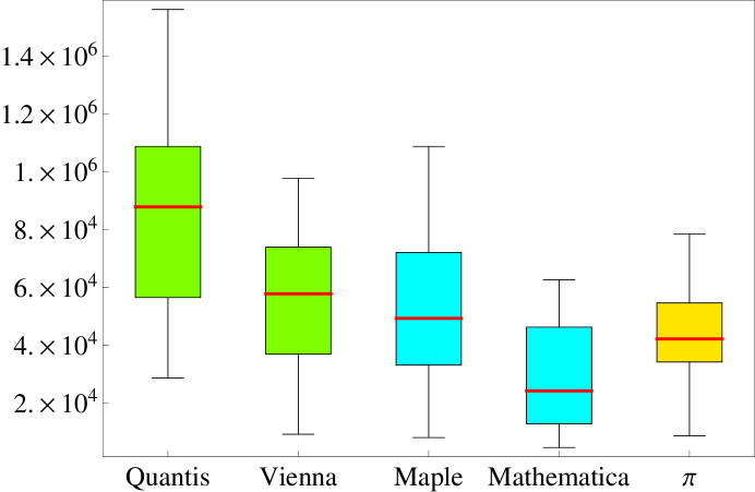
Figure 1: (Color online) Box-and-whisker plot for the results of the “book stack” randomness test.

Table 1: Statistics for the results of the “book stack” randomness test.

Descriptive statistics	min	Q1	median	Q3	max	mean	sd
Maple	7964	34490	49220	69630	108700	53410	33068.58
Mathematica	4508	13020	24110	43450	62570	27940	19406.03
Quantis	28600	60480	87780	106700	156100	89990	41545.76
Vienna	9110	38420	57720	73220	97660	53860	27938.92
$\pi$	8551	35480	42100	52870	78410	41280	20758.46

IV.2 Solovay-Strassen probabilistic primality test

The second algorithmic test, based on the Solovay-Strassen probabilistic primality test, uses Carmichael (composite) numbers which are “difficult” to factor, to determine the quality of randomness by computing how fast the probabilistic primality test reaches the verdict “composite” Solovay and Strassen (1977); Chaitin and Schwartz (1978). All Carmichael numbers less than $10^{16}$ have been used Pinch (1998, 2007).

To test whether a positive integer $n$ is prime, we take $k$ natural numbers uniformly distributed between 1 and $n-1$, inclusive, and, for each one $i$, check whether the predicate $W(i,n)$ holds. If this is the case we say that “$i$ is a witness of $n$’s compositeness”. If $W(i,n)$ holds for at least one $i$ then $n$ is composite; otherwise, the test is inconclusive, but in this case if one declares $n$ to be prime then the probability to be wrong is smaller than $2^{-k}$.

This is due to the fact that at least half $i$’s from $1$ to $n-1$ satisfy $W(i,n)$ if $n$ is indeed composite, and none of them satisfy $W(i,n)$ if $n$ is prime Solovay and Strassen (1977). Selecting $k$ natural numbers between 1 and $n-1$ is the same as choosing a binary string $s$ of length $n-1$ with $k$ $1$’s such that the $i$th bit is 1 iff $i$ is selected. Ref. Chaitin and Schwartz (1978) contains a proof that, if $s$ is a long enough algorithmically random binary string, then $n$ is prime iff $Z(s,n)$ is true, where $Z$ is a predicate constructed directly from conjunctions of negations of $W$ .

A Carmichael number is a composite positive integer $k$ satisfying the congruence $b^{k-1}\equiv 1({\rm mod}\,k)$ for all integers $b$ relative prime to $k$. Carmichael numbers are composite, but are difficult to factorize and thus are “very similar” to primes; they are sometimes called pseudo-primes. Carmichael numbers can fool Fermat’s primality test, but less the Solovay-Strassen test. With increasing values, Carmichael numbers become “rare” .

The fourth test uses Solovay-Strassen probabilistic primality test for Carmichael numbers (composite) with prefixes of the sample strings as the binary string $s$. We used the Solovay-Strassen test for all Carmichael numbers less than $10^{16}$—computed in Ref. Pinch (1998, 2007)—with numbers selected according to increasing prefixes of each sample string till the algorithm returns a non-primality verdict. The metric is given by the length of the sample used to reach the correct verdict of non-primality for all of the 246683 Carmichael numbers less than $10^{16}$. [We started with $k=1$ tests (per each Carmichael number) and increase $k$ until the metric goal is met; as $k$ increases we always use new bits (never recycle) from the sample source strings.] The results are presented in Figure 2 and Table 2.

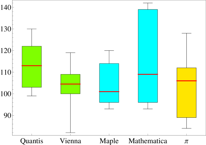
Figure 2: (Color online) Box-and-whisker plot for the results based on the Solovay-Strassen probabilistic primality test.

Table 2: Statistics for the results based on the Solovay-Strassen probabilistic primality test.

Descriptive statistics	min	Q1	median	Q3	max	mean	sd
Maple	93.0	96.0	101.0	113.5	120.0	104.9	10.57723
Mathematica	93.0	97.0	109.0	132.3	142.0	113.5	19.60867
Quantis	99.0	103.3	113.0	121.3	130.0	112.6	10.66875
Vienna	82.0	100.3	104.5	109.0	119.0	103.5	11.03781
$\pi$	84.0	91.75	106.0	110.8	128.0	104.7	10.66875

IV.3 Borel normality test

Borel normality — requesting that every binary string appears in the sequence with the correct probability $2^{-n}$ for a string of length $n$ — served as the first mathematical definition of randomness Borel (1909). A sequence is (Borel) normal if every binary string appears in the sequence with the right probability (which is $2^{-n}$ for a string of length $n$). A sequence is normal if and only it is incompressible by any information lossless finite-state compressor Ziv and Lempel (1978), so normal sequences are those sequences that appear random to any finite-state machine.

Every algorithmic random infinite sequence is Borel normal Calude (1994). The converse implication is not true: there exist computable normal sequences (e.g., Champernowne’s constant).

Normality is invariant under finite variations: adding, removing, or changing a finite number of bits in any normal sequence leaves it normal. Further, if a sequence satisfies the normality condition for strings of length $n+1$, then it also satisfies normality for strings of length $n$, but the converse is not true.

Normality was transposed to strings in Ref. Calude (1994). In this process one has to replace limits with inequalities. As a consequence, the above two properties, which are valid for sequences, are no longer true for strings.

For any fixed integer $m>1$, consider the alphabet $B_{m}=\{0,1\}^{m}$ consisting of all binary strings of length $m$, and for every $1\leq i\leq 2^{m}$ denote by $N_{i}^{m}$ the number of occurrences of the lexicographical $i$th binary string of length $m$ in the string $x$ (considered over the alphabet $B_{m}$). By $|x|_{m}$ we denote the length of $x$. A string $x$ is Borel normal if for every natural $1\leq m\leq\log_{2}\log_{2}|x|,$

$$\left|\frac{N_{j}^{m}(x)}{|x|_{m}}-2^{-m}\right|\leq\sqrt{\frac{\log_{2}|x|}{|x|}}\raisebox{2.15277pt}{,}$$

for every $1\leq j\leq 2^{m}$. In Ref. Calude (1994) it is shown that almost all algorithmic random strings are Borel normal.

In the first test we count the maximum, minimum and difference of non-overlapping occurrences of $m$-bit ($m=1,\ldots,5$) strings in each sample string. Then we tested the Borel normality property for each sample string and found that almost all strings pass the test, with some notable exceptions. We found that several of the Vienna sequences failed the expected count range for $m=2$ and a few of the Vienna sequences were outside the expected range for $m=3$ and $m=4$ (some less then the expected minimum count and some more than the expected maximum count). The only other bit sequence that was outside the expected range count was one of the Mathematica sequences that had a too big of a count for $k=1$. Figure 3 depicts a box-and-whisker plot of the results. This is followed by statistical (numerical) details in Table 3.

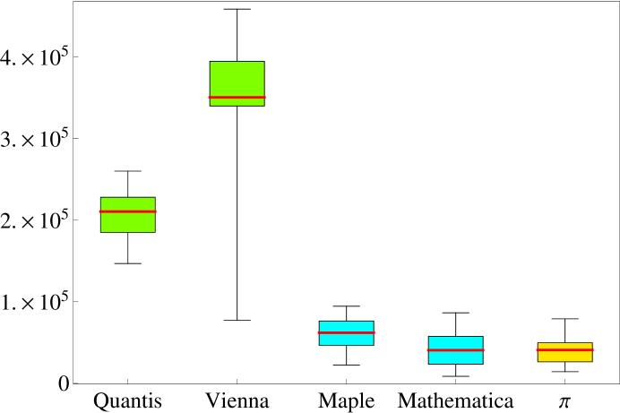
Figure 3: (Color online) Box-and-whisker plot for the results for tests of the Borel normality property.

Table 3: Statistics for the results for tests of the Borel normality property.

Descriptive statistics	min	Q1	median	Q3	max	mean	sd
Maple	22430	47170	61990	76130	94510	60210	21933.52
Mathematica	8572	25500	40590	55650	86430	41870	23229.77
Quantis	146800	185100	210500	226600	260000	207200	33515.65
Vienna	77410	340200	350500	392500	260000	337100	103354.3
$\pi$	14260	28860	40880	47860	79030	40220	17906.21

IV.4 Test based on Shannon’s information theory

The next test computes “sliding window” estimations of the Shannon entropy $L_{n}^{1},\ldots,L_{n}^{t}$ according to the method described in Wyner (1994): a smaller entropy is a symptom of less randomness. The results are presented in Figure 4 and Table 4.

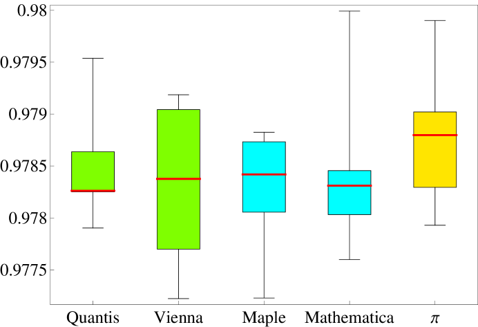
Figure 4: (Color online) Box-and-whisker plot for average results in “sliding window” estimations of the Shannon entropy.

Table 4: Statistics for average results in “sliding window” estimations of the Shannon entropy.

Descriptive statistics	min	Q1	median	Q3	max	mean	sd
Maple	0.9772	0.9781	0.9784	0.9787	0.9788	0.9783	0.0005231617
Mathematica	0.9776	0.9781	0.9783	0.9785	0.9800	0.9783	0.0006654936
Quantis	0.9779	0.9783	0.9783	0.9786	0.9795	0.9784	0.0004522699
Vienna	0.9772	0.9777	0.9784	0.9790	0.9792	0.9783	0.0006955834
$\pi$	0.9779	0.9784	0.9788	0.9790	0.9799	0.9788	0.0006062724

IV.5 Test based on random walks

A symptom of non-randomness of a string is detected when the plot generated by viewing a sample sequence as a 1D random walk meanders “less away” from the starting point (both ways); hence the max-min range is the metric.

The fifth test is thus based on viewing a random sequence as a one-dimensional random walk; whereby the successive bits, associated with an increase of one unit per bit of the $x$-coordinate, are interpreted as follows: $1=$“move up,” and $0=$“move down” on the $y$-axis. In this way a measure is obtained for how far away one can reach from the starting point (in either positive or negative) from the starting $y$-value of $0$ that one can reach using successive bits of the sample sequence. Figure 5 and Table 5 summarize the results.

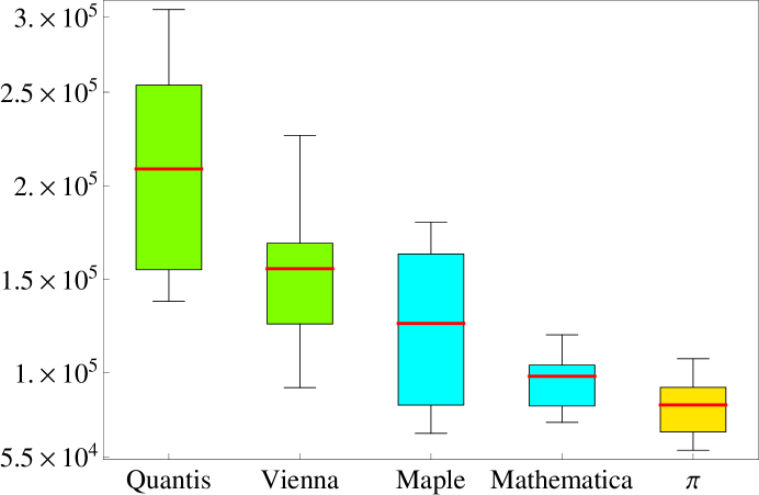
Figure 5: (Color online) Box-and-whisker plot for the results of the random walk tests.

Table 5: Statistics for the results of the random walk tests.

Descriptive statistics	min	Q1	median	Q3	max	mean	sd
Maple	67640	88730	126400	162500	180500	125300	42995.59
Mathematica	73500	84760	98110	103400	120300	96450	14685.34
Quantis	138200	161600	209000	250200	294200	211300	55960.23
Vienna	92070	130200	155600	167600	226900	152900	36717.55
$\pi$	58570	70420	82800	91920	107500	82120	14833.75

V Statistical analysis of randomness tests results

In what follows the significance of results corresponding to each randomness test applied to all five sources have been analyzed by means of some statistical comparison tests. The Kolmogorov-Smirnov test for two samples Conover (1999) determines if two datasets differ significantly. This test has the advantage of making no prior assumption about the distribution of data; i.e., it is non-parametric and distribution free.

The Kolmogorov-Smirnov test returns a $p$-value, and the decision “the difference between the two datasets is statistically significant” is accepted if the $p$-value is less than $0.05$; or, stated pointedly, if the probability of taking a wrong decision is less than $0.05$. Exact $p$-values are only available for the two-sided two-sample tests with no ties.

In some cases we have tried to double-check the decision “no significant differences between the datasets” at the price of a supplementary, plausible distribution assumption. Therefore, we have performed the Shapiro-Wilk test for normality Shapiro and Wilk (2005) and, if normality is not rejected, we have assumed that the datasets have normal (Gaussian) distributions. In order to be able to compare the expected values (means) of the two samples, the Welch $t$-test Welch (1947), which is a version of Student’s test, has been applied. In order to emphasize the relevance of p-values less than 0.05 associated with Kolmogorov-Smirnov, Shapiro-Wilk and Welch’s $t$-tests, they are printed in boldface and discussed in the text.

V.1 Book stack randomness test

The results of the Kolmogorov-Smirnov test associated with the “book-stack” tests are enumerated in Table 6. Statistically significant differences are identified for Quantis versus Mathematica and $\pi$.

Table 6: Kolmogorov-Smirnov test for the “book-stack” tests.

Kolmogorov-Smirnov test $p$-values	Mathematica	Quantis	Vienna	$\pi$
Maple	0.4175	0.1678	0.9945	0.4175
Mathematica		0.0021	0.1678	0.4175
Quantis			0.1678	0.0123
Vienna				0.4175

As more compression is a symptom of less randomness, the corresponding ranking of samples is as follows: $\langle\text{Quantis}\rangle=89988.9>\langle\text{Vienna}\rangle=53863.8>\langle\text{Maple}\rangle=53411.6>\langle\pi\rangle=41277.5>\langle\text{Mathematica}\rangle=27938.3$. The Shapiro-Wilk tests results are presented in Table 7.

Table 7: Shapiro-Wilk test for the “book-stack” tests.

Shapiro-Wilk test	Maple	Mathematica	Quantis	Vienna	$\pi$
$p$-value	0.7880	0.4819	0.7239	0.8146	0.5172

Since normality is not rejected for any string, we apply the Welch’s $t$-test for the comparison of means. The results are enumerated in Table 8. Significant differences between the means are identified for the following sources: (i) Quantis versus all other sources (Maple, Mathematica, Vienna, $\pi$); and (ii) Vienna versus Mathematica and Maple (as already mentioned).

Table 8: Welch’s $t$-test for the “book-stack” tests.

$p$-value	Mathematica	Quantis	Vienna	$\pi$
Maple	0.0535	0.0436	0.974	0.3412
Mathematica		0.0009	0.0283	0.1551
Quantis			0.0368	0.0054
Vienna				0.2690

V.2 Solovay-Strassen probabilistic primality test

The Kolmogorov-Smirnov test results for this test are presented in Table 9, where no significant differences are detected.

The Shapiro-Wilk test results are presented in Table 10. Since there is no clear pattern of normality for the data, the application of Welch’s $t$-test is not appropriate.

Table 9: Kolmogorov-Smirnov test for the Solovay-Strassen tests.

Kolmogorov-Smirnov test $p$-values	Mathematica	Quantis	Vienna	$\pi$
Maple	0.7591	0.4005	0.7591	0.7591
Mathematica		0.7591	0.7591	0.7591
Quantis			0.4005	0.7591
Vienna				0.9883

Table 10: Shapiro-Wilk test for the Solovay-Strassen tests.

Shapiro-Wilk test	Maple	Mathematica	Quantis	Vienna	$\pi$
$p$-value	0.0696	0.0363	0.4378	0.6963	0.4315

V.3 Borel test of normality

The results of the Kolmogorov-Smirnov test are presented in Table 11.

Table 11: Kolmogorov-Smirnov test for the Borel normality tests.

Kolmogorov-Smirnov test $p$-values	Mathematica	Quantis	Vienna	$\pi$
Maple	0.4175	$\mathbf{<10^{-4}}$	0.0002	0.1678
Mathematica		$\mathbf{<10^{-4}}$	0.0002	0.9945
Quantis			0.0002	$\mathbf{<10^{-4}}$
Vienna				0.0002

Statistically significant differences are identified for (i) Quantis versus Maple, Maple, Mathematica and $\pi$; (ii) Vienna versus Maple, Mathematica and $\pi$; and (iii) Quantis versus Vienna.

Note that

1. Pseudo-random strings pass the Borel normality test for comparable, relatively small (with respect to quantum strings; cf. below), numbers of counts: if the angle brackets $\langle x\rangle$ stand for the statistical mean of tests on $x$, then $\langle\text{Maple}\rangle=60210$, $\langle\text{Mathematica}\rangle=41870$, $\langle\pi\rangle=40220$).

2. Quantum strings pass the Borel normality test only for “much larger numbers” of counts ($\langle\text{Quantis}\rangle=207200$, $\langle\text{Vienna}\rangle=337100$).

As a result, the Borel normality test detects and identifies statistically significantly differences between all pairs of computable and incomputable sources of “randomness.”

V.4 Test based on Shannon’s information theory

The results of the Kolmogorov-Smirnov test are presented in Table 12. No significant differences are detected. The descriptive statistics data for the results of this test indicates almost identical distributions corresponding to the five sources.

Table 12: Kolmogorov-Smirnov test for Shannon’s information theory tests.

Kolmogorov-Smirnov test $p$-values	Mathematica	Quantis	Vienna	$\pi$
Maple	0.7870	0.7870	0.7870	0.1678
Mathematica		0.7870	0.4175	0.0525
Quantis			0.4175	0.1678
Vienna				0.4175

The results of the Shapiro-Wilk test associated with a test based on Shannon’s information theory are presented in Table 13. Since there is no clear pattern of normality for the data, the application of Welch’s $t$-test is not appropriate.

Table 13: Shapiro-Wilk test for Shannon’s information theory tests.

Shapiro-Wilk test	Maple	Mathematica	Quantis	Vienna	$\pi$
$p$-value	0.1962	0.0189	0.0345	0.3790	0.8774

V.5 Test based on random walks

The Kolmogorov-Smirnov test results associated with test based on random walks are presented in Table 14. Statistically significant differences are identified for: (i) Quantis versus all other sources (Maple, Mathematica, Vienna and $\pi$); (ii) Vienna versus Mathematica, Vienna (as already mentioned) and $\pi$; and (iii) Maple versus $\pi$.

Quantum strings move farther away from the starting point than the pseudo-random strings; i.e., $\langle\text{{\it Quantis}}\rangle>\langle\text{{\it Vienna}}\rangle>\langle\text{{\it Maple}}\rangle>\langle\text{{\it Mathematica}}\rangle>\langle\pi\rangle$.

Table 14: Kolmogorov-Smirnov test for the random walk tests.

Kolmogorov-Smirnov test $p$-values	Mathematica	Quantis	Vienna	$\pi$
Mathematica	0.1678	0.0123	0.4175	0.0525
Quantis		$\mathbf{<10^{-4}}$	0.0021	0.1678
Vienna			0.0525	$\mathbf{<10^{-4}}$
$\pi$				0.0002

Note that quantum strings move farther away from the starting point than the pseudo-random strings; i.e., $\langle\text{{\it Quantis}}\rangle>\langle\text{{\it Vienna}}\rangle>\langle\text{{\it Maple}}\rangle>\langle\text{{\it Mathematica}}\rangle>\langle\pi\rangle$. It was quite natural to double-check the conclusion “Quantis and Vienna do not exhibit significant differences.” Hence we run the Shapiro-Wilk test, which concludes that normality is not rejected; cf. Table 15.

Table 15: Shapiro-Wilk test for the random walk tests.

Shapiro-Wilk test	Maple	Mathematica	Quantis	Vienna	$\pi$
$p$-value	0.2006	0.9268	0.5464	0.8888	0.9577

Next, we apply the Welch’s $t$-test for the comparison of means. The results are given in Table 16. Significant differences between the means are identified for the following sources: (i) Quantis versus all other sources (Maple, Quantis, Vienna, $\pi$); (ii) Vienna versus Mathematica), Quantis (as already mentioned) and $\pi$; (iii) Maple versus $\pi$.

Table 16: Welch’s $t$-tests for the random walk tests.

$p$-value	Mathematica	Quantis	Vienna	$\pi$
Maple	0.06961	0.0013	0.1409	0.0119
Mathematica		$\mathbf{<10^{-4}}$	0.0007	0.0435
Quantis			0.0143	$\mathbf{<10^{-4}}$
Vienna				0.0001

VI Summary

Tests based on algorithmic information theory analyze algorithmic randomness, the strongest possible form of incomputability. In this respect they differ from tests employed in the standard test batteries, as the former depend on irreducible algorithmic information content, which is constant for algorithmic pseudo-random generators. Thus the set of randomness tests performed for our analysis could in principle be expected to be “more sensitive” with respect to differentiating between quantum randomness and algorithmic types of “quasi-randomness” than statistical tests alone.

All tests have produced evidence — with different degrees of statistical significance — of differences between quantum and non-quantum sources. In summary:

1. For the test for Borel normality — the strongest discriminator test — statistically significant differences between the distributions of datasets are identified for (i) Quantis versus Maple, Mathematica and $\pi$; (ii) Vienna versus Maple, Mathematica and $\pi$; and (iii) Quantis versus Vienna.

   Not only that the average number of counts is larger for quantum sources, but the increase is quite significant: Quantis is $3.5-5$ times larger than the corresponding average number of counts for software-generated sources, and Vienna is $5-8$ times larger than those values.

2. For the test based on random walks, statistically significant differences between the distributions of datasets are identified for: (i) Quantis versus all other sources (Maple, Mathematica, Vienna and $\pi$); (ii) Vienna versus Mathematica, Vienna and $\pi$. Quantum strings move farther away from the starting point than the pseudo-random strings; i.e., $\langle\text{{\it Quantis}}\rangle>\langle\text{{\it Vienna}}\rangle>\langle\text{{\it Maple}}\rangle>\langle\text{{\it Mathematica}}\rangle>\langle\pi\rangle$.

3. For the “book-stack” test, significant differences between the means are identified for the following sources: (i) Quantis versus all other sources (Maple, Mathematica, Vienna, $\pi$); and (ii) Vienna versus Mathematica and Maple.

4. For the test based on Shannon’s information theory, as well as for the Solovay-Strassen test, no significant differences among the five chosen sources are detected. In the first case the reason may come from the fact that averages are the same for all samples. In the second case the reason may be due to the fact that the test is based solely on the behavior of algorithmic random strings and not on a specific property of randomness.

We close with a cautious remark about the impossibility to formally or experimentally “prove absolute randomness.” Any claim of randomness can only be secured relative to, and with respect to, a more or less large class of laws or behaviors, as it is impossible to inspect the hypothesis against an infinity of — and even less so all — conceivable laws. To rephrase a statement about computability (Davis, 1958, p. 11), “how can we ever exclude the possibility of our presented, some day (perhaps by some extraterrestrial visitors), with a (perhaps extremely complex) device that “computes” and “predicts” a certain type of hitherto “random” physical behavior?”

References

- Born (1926) Max Born, “Zur Quantenmechanik der Stoßvorgänge,” Zeitschrift für Physik, 37, 863–867 (1926a).
- Born (1926) Max Born, “Quantenmechanik der Stoßvorgänge,” Zeitschrift für Physik, 38, 803–827 (1926b).
- Zeilinger (2005) Anton Zeilinger, “The message of the quantum,” Nature, 438, 743 (2005).
- Calude and Svozil (2008) Cristian S. Calude and Karl Svozil, “Quantum randomness and value indefiniteness,” Advanced Science Letters, 1, 165–168 (2008), arXiv:quant-ph/0611029 .
- Martin-Löf (1966) Per Martin-Löf, “The definition of random sequences,” Information and Control, 9, 602–619 (1966), ISSN 0019-9958.
- Chaitin (2001) Gregory J. Chaitin, Exploring Randomness (Springer Verlag, London, 2001).
- Calude (2002) Cristian Calude, Information and Randomness—An Algorithmic Perspective, 2nd ed. (Springer, Berlin, 2002).
- Svozil (1990) Karl Svozil, “The quantum coin toss—testing microphysical undecidability,” Physics Letters A, 143, 433–437 (1990).
- Rarity et al. (1994) J. G. Rarity, M. P. C. Owens, and P. R. Tapster, “Quantum random-number generation and key sharing,” Journal of Modern Optics, 41, 2435–2444 (1994).
- Jennewein et al. (2000) Thomas Jennewein, Ulrich Achleitner, Gregor Weihs, Harald Weinfurter, and Anton Zeilinger, “A fast and compact quantum random number generator,” Review of Scientific Instruments, 71, 1675–1680 (2000), quant-ph/9912118 .
- Stefanov et al. (2000) André Stefanov, Nicolas Gisin, Olivier Guinnard, Laurent Guinnard, and Hugo Zbinden, “Optical quantum random number generator,” Journal of Modern Optics, 47, 595–598 (2000).
- Hai-Qiang et al. (2004) Ma Hai-Qiang, Wang Su-Mei, Zhang Da, Chang Jun-Tao, Ji Ling-Ling, Hou Yan-Xue, and Wu Ling-An, “A random number generator based on quantum entangled photon pairs,” Chinese Physics Letters, 21, 1961–1964 (2004).
- Wang et al. (2006) P. X. Wang, G. L. Long, and Y. S. Li, “Scheme for a quantum random number generator,” Journal of Applied Physics, 100, 056107 (2006).
- Fiorentino et al. (2007) M. Fiorentino, C. Santori, S. M. Spillane, R. G. Beausoleil, and W. J. Munro, “Secure self-calibrating quantum random-bit generator,” Physical Review A (Atomic, Molecular, and Optical Physics), 75, 032334 (2007).
- Svozil (2009) Karl Svozil, “Three criteria for quantum random-number generators based on beam splitters,” Physical Review A (Atomic, Molecular, and Optical Physics), 79, 054306 (2009), arXiv:0903.2744 .
- Marsaglia (1995) George Marsaglia, “The Marsaglia random number CDROM including the diehard battery of tests of randomness,” (1995).
- Rukhin et al. (2001) Andrew Rukhin, Juan Soto, James Nechvatal, Miles Smid, Elaine Barker, Stefan Leigh, Mark Levenson, Mark Vangel, David Banks, Alan Hekert, James Dray, and San Vo, A Statistical Test Suite for Random and Pseudorandom Number Generators for Cryptographic Applications. NIST Special Publication 800-22 (National Institute of Standards and Technology (NIST), 2001).
- L’Ecuyer and Simard (2007) Pierre L’Ecuyer and Richard Simard, “Testu01: A C library for empirical testing of random number generators,” ACM Transactions on Mathematical Software (TOMS), 33, 22 (2007), ISSN 0098-3500.
- ID Quantique SA (2001-2010) ID Quantique SA, QUANTIS. Quantum number generator (idQuantique, Geneva, Switzerland, 2001-2010).
- Institut für Quantenoptik und Quanteninformation (2003) (IQOQI) Institut für Quantenoptik und Quanteninformation (IQOQI), Quantum number generator (2003) personal communication.
- Wolfram Research, Inc. (2007) Wolfram Research, Inc., Mathematica Edition: Version 6.0. Mathematica random generator. ExtendedCA default.” (Wolfram Research, Inc., Waterloo, Ontario, 2007).
- Maplesoft (2007) Maplesoft, Maple Edition: Version 11. Maple random generator (Maplesoft, Champaign, Illinois, 2007).
- Kanada and Takahashi (1995) Yasumasa Kanada and Daisuke Takahashi, “Calculation of up to 4,294,960,000 decimal digits,” (1995).
- von Neumann (1951) John von Neumann, “Various techniques used in connection with random digits,” National Bureau of Standards Applied Math Series, 12, 36–38 (1951), reprinted in John von Neumann, Collected Works, (Vol. V), A. H. Traub, editor, MacMillan, New York, 1963, p. 768–770.
- Borel (1909) Émile Borel, “Les probabilités dénombrables et leurs applications arithmétiques,” Rendiconti del Circolo Matematico di Palermo (1884 - 1940), 27, 247–271 (1909).
- Hertling (2002) P. Hertling, “Simply normal numbers to different bases,” Journal of Universal Computer Science, 8, 235–242 (2002).
- Calude et al. (2009) Cristian S. Calude, Michael J. Dinneen, Monica Dumitrescu, and Karl Svozil, How Random Is Quantum Randomness? (Extended Version), Report CDMTCS-372 (Centre for Discrete Mathematics and Theoretical Computer Science, University of Auckland, Auckland, New Zealand, 2009) arXiv:0912.4379 .
- Ryabko and Pestunov (2004) B. Ya. Ryabko and A. I. Pestunov, ““Book stack” as a new statistical test for random numbers,” Problemy Peredachi Informatsii, 40, 73–78 (2004), ISSN 0555-2923.
- Ryabko and Monarev (2005) B. Ya. Ryabko and V. A. Monarev, “Using information theory approach to randomness testing,” J. Statist. Plann. Inference, 133, 95–110 (2005), ISSN 0378-3758.
- Solovay and Strassen (1977) Robert Solovay and Volker Strassen, “A fast Monte-Carlo test for primality,” SIAM Journal on Computing, 6, 84–85 (1977), corrigendum in Ref. Solovay and Strassen (1978).
- Chaitin and Schwartz (1978) Gregory J. Chaitin and Jacob T. Schwartz, “A note on monte Carlo Primality tests and algorithmic information theory,” Communications on Pure and Applied Mathematics, 31, 521–527 (1978).
- Pinch (1998) Richard G.E. Pinch, “The Carmichael numbers up to ,” (1998), arXiv:math.NT/9803082 .
- Pinch (2007) Richard G.E. Pinch, “The Carmichael numbers up to ,” in Proceedings of Conference on Algorithmic Number Theory 2007. TUCS General Publication No 46, edited by Anne-Maria Ernvall-Hytönen, Matti Jutila, Juhani Karhumäki, and Arto Lepistö (Turku Centre for Computer Science, Turku, Finland, 2007) pp. 129–131.
- Note (1) In fact, every “decent” Monte Carlo simulation algorithm in which tests are chosen according to an algorithmic random string produces a result which is not only true with high probability, but rigorously correct Calude and Zimand (1984).
- Note (2) There are 1,401,644 Carmichael numbers in the interval .
- Ziv and Lempel (1978) J. Ziv and A. Lempel, “Compression of individual sequences via variable-rate coding,” IEEE Transactions on Information Theory, 24, 530–536 (1978).
- Calude (1994) Cristian Calude, “Borel normality and algorithmic randomness,” in Developments in Language Theory, edited by Grzegorz Rozenberg and Arto Salomaa (World Scientific, Singapore, 1994) pp. 113–129, ISBN 981-02-1645-9.
- Wyner (1994) Aaron D. Wyner, “Shannon lecture: Typical sequences and all that: Entropy, pattern matching, and data compression,” IEEE Information Theory Society (1994).
- Conover (1999) William J. Conover, Practical Nonparametric Statistics (John Wiley & Sons, New York, 1999) p. 584.
- Shapiro and Wilk (2005) S. S. Shapiro and M. B. Wilk, “An analysis of variance test for normality (complete samples),” Biometrika, 52, 591–611 (2005).
- Welch (1947) B. L. Welch, “The generalization of “student’s” problem when several different population variances are involved,” Biometrika, 34 (1947), doi:10.1093/biomet/34.1-2.28.
- Davis (1958) Martin Davis, Computability and Unsolvability (McGraw-Hill, New York, 1958).
- Solovay and Strassen (1978) Robert Solovay and Volker Strassen, “Erratum: A fast Monte-Carlo test for primality,” SIAM Journal on Computing, 7, 118 (1978).
- Calude and Zimand (1984) Cristian Calude and Marius Zimand, “A relation between correctness and randomness in the computation of probabilistic algorithms,” Internat. J. Comput. Math., 16, 47–53 (1984), ISSN 0020-7160.