Use of $\delta N$ formalism
- Difficulties in generating large local-type non-Gaussianity during inflation -

Abstract

We discuss generation of non-Gaussianity in density perturbation through the super-horizon evolution during inflation by using the so-called $\delta N$ formalism. We first provide a general formula for the non-linearity parameter generated during inflation. We find that it is proportional to the slow-roll parameters, multiplied by the model dependent factors that may enhance the non-Gaussianity to the observable ranges. Then we discuss three typical examples to illustrate how difficult to generate sizable non-Gaussianity through the super-horizon evolution during inflation. First example is the double inflation model, which shows that temporal violation of slow roll conditions is not enough for the generation of non-Gaussianity. Second example is the ordinary hybrid inflation model, which illustrates the importance of taking into account perturbations on small scales. Finally, we discuss Kadota-Stewart model. This model gives an example in which we have to choose rather unnatural initial conditions even if large non-Gaussianity can be generated.

1 Introduction: Success of inflation

Inflation solved the various cosmological problems like horizon, homogeneity, flatness problem, just by assuming that the potential energy of scalar fields dominates the expansion of the universe. Moreover, inflation scenario naturally explains the origin of the almost scale invariant density perturbation. The observations in the past decades verified many of the predictions of inflation. Almost scale invariant spectrum is now confirmed and now we even know that the violation of the exact scale invariance is 4% level [1], which is also consistent with the simplest slow roll inflation scenario.

1.1 Density perturbation

The amplitude of quantum fluctuation of inflaton $\phi$ during slow-roll inflation is determined by the unique relevant mass scale at that time, e.g. the Hubble rate $H$:

$$\delta\phi={H\over 2\pi}.$$ (1)

However, on scales as large as the Horizon radius the meaning of the amplitude of field perturbation becomes subtle because it depends on the choice of gauge. For the flat slicing gauge, in which the trace of the spatial curvature is kept unperturbed, the perturbation equation for a scalar field becomes very simple and looks very similar to the one without gravitational perturbation [2]. Therefore the amplitude mentioned above can be in fact understood as that in the flat slicing gauge. This amplitude of perturbation can be interpreted as the dimensionless curvature perturbation on a uniform energy density surface $\zeta$. Transformation law is given by

$$\zeta=H\delta t=H{\delta\phi\over\dot{\phi}}={H^{2}\over 2\pi\dot{\phi}},$$ (2)

where $\delta t$ is the shift in time coordinate for this transformation, which is given by $\delta\phi/\dot{\phi}$ using the time derivative of the background scalar field. Writing the perturbation amplitude in terms of $\zeta$ is useful because the curvature perturbation does not evolve on super-horizon scales when the evolution path of the universe is unique. This constancy of $\zeta$ simplifies the analysis of density perturbation during inflation for a single inflaton model. An extension of this argument to the case of multi-component inflaton is the $\delta N$ formalism [3, 4, 5, 6, 7, 8], as we explain below.

1.2 Further steps from observations

Further detailed comparison between the theoretical predictions and future observations is awaited. One important observation will be tensor-type perturbation in cosmic microwave background. Tensor-type perturbation is the transverse-traceless part of the spatial metric perturbation, which is generated by the same mechanism as the perturbation of the inflaton field. Gravitational action has a overall prefactor $m_{pl}^{2}$, and hence we define the canonically normalised metric perturbation $\psi_{\mu\nu}=m_{pl}\delta g_{\mu\nu}$ so as to absorb this factor from the quadratic action. Then, the quadratic action for the transverse traceless part of $\psi_{\mu\nu}$ becomes identical to the one for a massless scalar field. Therefore the amplitude of perturbation $\psi_{\mu\nu}$ generated through almost de Sitter inflation is also $O(H)$. Using this relation, we have

$$\left|{\delta T\over T}\right|_{tensor}=O(\delta g_{\mu\nu})=O\left({\psi_{\mu\nu}\over m_{pl}}\right)=O\left({H\over m_{pl}}\right).$$ (3)

Thus we find that the CMB temperature fluctuation caused by the tensor perturbation directly probes the value of $H$ during inflation, i.e. the energy scale of inflation. This can be discriminated from the scalar-type perturbation by looking at B-mode polarisation [9, 10, 11].

Another important observation is the non-Gaussianity of the temperature fluctuations [12, 13]. The non-Gaussianity is caused by the non-linear dynamics of cosmological perturbation. Once we have completely understood the evolution of density perturbation at late time, the remaining non-Gaussianity which is not accounted for should have their origin in the earlier universe. The results of WMAP 7 years indicate that the local-type non-Gaussianity parameter is given as $f_{NL}=32\pm 21$ at 68% confidence level [1]. For the Planck satellite, it is expected that the window of $f_{{\rm NL}}$ is expected to be reduced to $O(10)$ [9].

Recently, non-Gaussianity of the primordial perturbation also has been studied by many authors  [7, 8, 12, 13, 14, 15, 16, 17, 18, 19, 20, 21, 22, 23, 24, 25, 26, 27, 28, 29, 30, 31, 32, 33, 34, 35, 36, 37, 38, 39, 40, 41, 42, 43, 44, 45, 46, 47, 48]. The main reason for non-Gaussianity to attract much attention is the expectation to future observations mentioned above. These observations may bring us valuable information about the dynamics of inflation. Here in this short paper, we would like to clarify the difficulties in generating large non-Gaussianity from the non-linear dynamics during inflation.

2 Basic feature of generation of non-Gaussianity of local-type.

2.1 Local non-Gaussianity

Primordial non-Gaussianity gives rise as non-trivial higher order correlation functions in primordial perturbations. In principle, various types of non-Gaussianity are possibly generated [25, 26, 27], but here we focus on the so-called local-type non-Gaussianity. Local-type non-Gaussianity is characterised by the existence of one-to-one local map between the physical curvature perturbation $\zeta(x)$ and the variable which follows the Gaussian statistics $\zeta_{G}(x)$ at respective spatial points. Namely, we can expand the curvature perturbation as

$$\zeta(x)=\zeta_{G}(x)+{3\over 5}f_{NL}\zeta_{G}^{2}(x)+\cdots,$$ (4)

and the Gaussian variable $\zeta_{G}$ satisfies ordinary Gaussian statistics:

$$\left\langle\zeta^{G}_{{\bf k}_{1}}\zeta^{G}_{{\bf k}_{2}}\right\rangle=\delta^{(3)}({\bf k}_{1}+{\bf k}_{2})P_{\zeta}(k_{1}).$$ (5)

In this case three point function can be characterised by a single non-linear parameter $f_{NL}$ [12] as

$$\left\langle\zeta_{{\bf k}_{1}}\zeta_{{\bf k}_{2}}\zeta_{{\bf k}_{3}}\right\rangle=\delta^{(3)}({\bf k}_{1}+{\bf k}_{2}+{\bf k}_{3})B_{\zeta}(k_{1},k_{2},k_{3}),$$ (6)

with

$$\!\!\!B_{\zeta}(k_{1},k_{2},k_{3})={6\over 5}{f_{NL}\over(2\pi)^{3/2}}\Biggl{[}P_{\zeta}(k_{1})P_{\zeta}(k_{2})+P_{\zeta}(k_{2})P_{\zeta}(k_{3})+P_{\zeta}(k_{3})P_{\zeta}(k_{1})\Biggr{]}.$$ (7)

In general, other types of non-Gaussianity can be generated. However, when we focus on super-horizon dynamics, only local-type non-Gaussianity can be produced as is explained below.

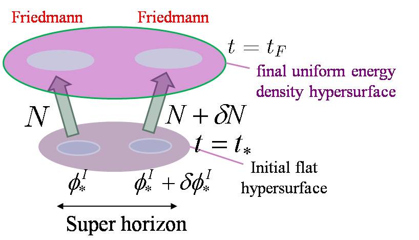
Figure 1: Schematic picture to explain $\delta N$ formalism.

2.2 Super-horizon dynamics

Here we just present an intuitive explanation about how the density perturbations evolve when the length scale is much larger than the Hubble scale. Super-horizon dynamics is locally described by the Friedmann-Robertson-Walker universe. We consider the evolution of the universe starting with an initial flat hypersurface at $t=t_{*}$, on which the initial values of the inflaton field have a certain distribution. We evolve the spacetime until reaching the final surface at $t=t_{F}$ that is characterised by a specified energy density as shown in Fig. 1. Hence, the final surface is a uniform energy density surface by definition. As each horizon patch is causally disconnected from the others in the inflating universe, its evolution is determined as a local process. If initial conditions are completely given in each horizon patch, we can solve the evolution of its future. Here, for simplicity, we assume that the evolution of the averaged values of fields in each horizon patch is determined by the averaged values of initial data. This assumption is not necessarily true in general, but we have a good reason to assume so in most cases. Initial conditions for the smaller scale perturbations can affect the evolution of the averaged values of variables. However, as there are so many small scale degrees of freedom, the average of their effects will not be largely fluctuated except for rare situations. Of course, even if we can neglect the effect of fluctuations on small scales, this does not mean that the backreaction due to small scale degrees of freedom does not modify the dynamics of the averaged values of variables. This backreaction effect arises at the second order perturbation or higher. Therefore the difference in the backreaction effect between different horizon patches is even higher order in perturbation. Thus, we usually neglect this effect for simplicity. Of course, in the situation like preheating the sub-horizon scale perturbations evolve more rapidly than the averaged values, we definitely need to take the backreaction into account. However, even in that case, it will not be necessary to know all the details of small scale perturbations to understand the evolution of the averaged variables.

Anyway, we neglect these effects originating from small scale perturbations here. Then, the e-folding number between the initial surface and the final one is completely determined by the initial averaged values of the variables. In the scalar field dominant universe, such initial conditions are specified by the values of the field components and their time derivatives, $\phi^{i}(t_{*},x)$ and $\dot{\phi}^{i}(t_{*},x)$. We denote $\phi^{i}(t_{*},x)$ together with $\dot{\phi}^{i}(t_{*},x)$ by $\phi^{I}(t_{*},x)$. Then, the e-folding number between the initial surface and the final one,

$$N(t_{F},t_{*},\phi^{I})\equiv\int_{t_{*}}^{t_{F}}Hdt$$ (8)

is given as a function of $\phi^{I}(t_{*},x)$. Then, roughly speaking, the spatial metric on the final uniform energy density surface will be given by

$$ds_{(3)}^{2}\approx e^{2N(t_{F},\phi^{I}(t_{*},x))}\delta_{ij}dx^{i}dx^{j},$$ (9)

The curvature perturbation is in fact the perturbation in the above exponent $N(t_{F},t_{*},\phi^{I}(t_{*},x))$, and hence we have

$$\zeta(t_{F})\approx\delta N(t_{F},\phi^{I}(t_{*},x)).$$ (10)

This formula is the heart of the $\delta N$ formalism [3, 4, 5, 6, 7, 8].

In the slow roll case, the evolution equation for the scalar field can be approximated by a first order differential equation in $t$. Therefore the phase space of the initial conditions $\phi^{I}(t_{*},x)$ is reduced to $\phi^{i}(t_{*},x)$. In this case, if there is only a single component, the trajectory in the field configuration space, which is one dimensional, is necessarily unique. Then, $\delta N(t_{F},\phi^{i}(t_{*},x))$ does not depend on the choice of the energy density of the final surface. It can be set to a representative background value at the initial time. Namely,

$$\delta N(t_{F},\phi^{i}(t_{*},x))=\delta N(t_{*},\phi^{I}(t_{*},x)).$$ (11)

Therefore nothing non-trivial happens during the super-horizon evolution for slow-roll single field inflation. Even if the slow-roll conditions are violated, single field inflation does not produce sizable $\delta N$ for modes far beyond the horizon scale. This is because the trajectories in the configuration space continues to converge as the decaying perturbation mode gets irrelevant. In order to generate non-Gaussianity through the evolution on super horizon scales, it is therefore essential to consider multi-component inflaton field.

Using the formula (10), we can express the curvature perturbations on the final surface in terms of the field perturbations on the initial surface as

$$\zeta(t_{c})=\delta N=N^{*}_{I}\delta\phi^{I}_{*}+{1\over 2}N^{*}_{IJ}\delta\phi^{I}_{*}\delta\phi^{J}_{*}+\cdots,$$ (12)

where the subscript $*$ indicates the quantities evaluated at $\phi^{I}=\bar{\phi}^{I}(t_{*})$, and the subscript $I$ associated with $N$ means the differentiation with respect to $\phi^{I}(t_{*})$:

$$N_{I}^{*}\equiv\left.{\partial N(t_{c},\phi^{I})\over\partial\phi^{I}}\right|_{\phi=\bar{\phi}(t_{*})},\qquad N_{IJ}^{*}\equiv\left.{\partial^{2}N(t_{c},\phi^{I})\over\partial\phi^{I}\partial\phi^{J}}\right|_{\phi=\bar{\phi}(t_{*})},$$ (13)

where $\bar{\phi}^{I}(t)$ is the background trajectory. With the aid of Eq. (12), we can write the three point correlation function of $\zeta$ at $t=t_{F}$ as

$$\left\langle\zeta({\bf x}_{1})\zeta({\bf x}_{2})\zeta({\bf x}_{3})\right\rangle = N^{*}_{I}N^{*}_{J}N^{*}_{K}\left\langle\delta\phi_{*}^{I}({\bf x}_{1})\delta\phi_{*}^{J}({\bf x}_{2})\delta\phi_{*}^{K}({\bf x}_{3})\right\rangle$$ (16)

$$+N^{*}_{I}N^{*}_{J}N^{*}_{KL}\Bigl{[}\left\langle\delta\phi_{*}^{I}({\bf x}_{1})\delta\phi_{*}^{J}({\bf x}_{2})\delta\phi_{*}^{K}({\bf x}_{3})\delta\phi_{*}^{L}({\bf x}_{3})\right\rangle$$

$$\qquad\qquad\qquad\qquad+(3{\rm perms})\Bigr{]}+\cdots.$$

The first term contains only three $\delta\phi$s. If the initial fluctuations at $t=t_{*}$ are Gaussian, this term vanishes. Depending on the model of inflation, early generation of non-Gaussianity at around horizon crossing is possible [26]. However, the observed almost scale invariant and slightly red spectrum of initial curvature perturbation strongly suggests that the inflation is likely to have been in the slow roll regime at around the horizon crossing. For the slow roll inflation, it is shown that the early production of non-Gaussianity is strongly suppressed [14, 15, 16]. Therefore, it is well motivated to consider non-Gaussianity contained in the second term (or even higher order terms), generated by the non-linear evolution after the horizon crossing.

Generation of non-Gaussianity can be classified into two classes. One is generation through the super horizon evolution during inflation. The other is generation at the end of or after inflation [29, 30, 31, 34, 35, 36, 37, 43, 44]. In either case the non-Gaussianity is of local type. Three point correlation function is characterised by one parameter $f_{NL}$ alone, and it is related to the e-folding number $N(t_{F},\phi^{I})$ as

$${6\over 5}f_{NL}\approx{N^{I}_{*}N^{J}_{*}N^{*}_{IJ}\over(N^{K}_{*}N^{*}_{K})^{2}},$$ (17)

neglecting higher order terms.

3 Non-Gaussianity produced at the end of or after inflation

There are various models of inflation that produces large non-Gaussianity of local type at the end of or after inflation. Here we briefly mention curvaton type model [51, 52] as a typical example to explain the mechanism to generate large non-Gaussianity. Curvaton is another scalar field that is introduced to explain the origin of primordial curvature perturbation. During inflation, curvaton field is almost massless but it starts to behave as a massive field later when the Hubble rate decays down to the mass scale of the curvaton field. Then, the curvaton starts to oscillate around the minimum of the potential and eventually decays into radiation. At this point, the fluctuations in the curvaton $\sigma$ are transferred into curvature perturbations. For simplicity, we consider the case that the density perturbations are dominated by the fluctuations originating from the curvaton. Neglecting a contribution of second order of $\delta\rho_{\sigma}$ to $\zeta$, which turns out to yield only $f_{NL}=O(1)$, we have [30]

$$\zeta={1\over 4}{\delta\rho_{\sigma}\over\rho}={r\over 4}\left(2{\delta\sigma\over\sigma}+\left({\delta\sigma\over\sigma}\right)^{2}\right),$$ (18)

where $r=\rho_{\sigma}/\rho_{tot}$ is the fraction of the energy density that the decay products of $\sigma$ takes. Here, we used the estimate $\rho_{\sigma}\approx m^{2}(\sigma+\delta\sigma)^{2}/2$ with $m$ being the mass of the curvaton.

The amplitude of the power spectrum is observationally fixed as

$$P_{\zeta}=O\left(\left[r{\delta\sigma/\sigma}\right]^{2}\right)=O(10^{-10}).$$ (19)

Therefore, if $\delta\sigma/\sigma$ is not small, $r$ can be as small as $10^{-5}$. On the other hand, the non-linear parameter is given by

$$f_{NL}=O\left({\langle\zeta^{3}\rangle/\langle\zeta^{2}\rangle^{2}}\right)=O\left({1/r}\right),$$ (20)

which can be as large as $10^{5}$. In this way, the production of large non-Gaussianity at the end of inflation is rather easily achieved.

As a mechanism for getting large non-Gaussianity, one can also consider generation of perturbations during preheating phase [49, 50, 43, 44, 45, 46, 47].In this case, the background evolution is strongly coupled to the evolution of small scale fluctuations because the e-folding number changes depending on how fast the energy of coherent oscillation of fields decays into the small scale perturbations. While in the other models the transmutation of homogeneous isocurvature perturbations on each Hubble patch into adiabatic perturbations is determined just by solving the background evolution of various homogeneous and isotropic universe models. In this sense the mechanism to generate density perturbation during preheating stage is quite different from the other models.

4 Non-Gaussianity produced during inflation

Here we just present the formula for $f_{NL}$ in slow-roll inflation with canonical kinetic term. A systematic derivation for more general formula, including higher order correlators, is given in Ref. [24]. Assuming that the initial perturbations of fields are Gaussian in the following form

$$\left\langle\delta\phi^{i}_{{\bf k}_{1}}\delta\phi^{j}_{{\bf k}_{2}}\right\rangle=\delta^{ij}\delta^{(3)}({\bf k}_{1}+{\bf k}_{2})P_{\delta\phi}(k_{1}),$$ (21)

the formula for $f_{NL}$ is written in terms of the potential of the scalar field $V$ as

$${6\over 5}f_{NL}=(N^{i}_{*}N_{i}^{*})^{-2}\int_{N_{*}}^{N_{F}}dN^{\prime}\,N_{j}(N^{\prime})Q^{j}_{kl}(N^{\prime})\Theta^{k}(N^{\prime})\Theta^{l}(N^{\prime}).$$ (22)

Here, we neglected non-Gaussianity in the relation between $\delta N$ and $\delta\phi^{i}$ at $N=N_{F}$. To define $N_{i}$ and $\Theta^{i}$, it is convenient to introduce the propagator

$$\Lambda^{i}_{j}(N,N^{\prime})=\left[T\exp\left(\int_{N^{\prime}}^{N}P(N^{\prime\prime})dN^{\prime\prime}\right)\right]{}^{i}_{j},$$ (23)

where

$$P^{i}_{j}(N)\equiv\left[-{V^{i}_{j}\over V}+{V^{i}V_{j}\over V^{2}}\right]_{\phi=\bar{\phi}(N)},$$ (24)

is the potential term that appears in the linear perturbation equation when we use the e-folding number $N$ as a time coordinate. The indices associated with $V$ represent differentiation with respect to scalar field. $T$ in Eq. (23) means that the matrices $P^{i}_{j}$ are ordered in time when the exponential is expanded in power of $P^{i}_{j}$. Using this propagator, $N_{i}$ and $\Theta^{i}$ are defined as

$$N_{i}(N)=N_{j}(N_{F})\Lambda^{j}_{i}(N_{F},N),$$ (25)

$$\Theta^{i}(N)\equiv\Lambda^{i}_{j}(N,N_{*})N^{j}_{*}.$$ (26)

$N_{i}(N)$ satisfies the equation of motion adjoint to the linear perturbation equation for $\delta\phi^{i}$,

$${d\over dN}N_{i}(N)=-P_{i}^{j}N_{j}(N),$$ (27)

with the boundary condition $N_{j}(N_{F})=(\partial N(N_{F},\phi^{i})/\partial\phi^{j})|_{\phi=\bar{\phi}(N_{F})}$. $\Theta^{i}(N)$ satisfies the same equation as $\delta\phi^{i}$

$${d\over dN}\Theta^{j}(N)=P_{i}^{j}\Theta^{i}(N),$$ (28)

and the boundary condition is given by $\Theta^{i}(N_{*})=N^{i}(N_{*})$, where the index is raised by the inverse of the field space metric, which is assumed to be $\delta^{ij}$ here. The three point interaction $Q^{i}_{jk}$ is given by

$$Q^{i}_{jk}(N)\equiv\left[-{V^{i}_{jk}\over V}+{V^{i}_{j}V_{k}\over V^{2}}+{V^{i}_{k}V_{j}\over V^{2}}+{V^{i}V_{jk}\over V^{2}}-2{V^{i}V_{j}V_{k}\over V^{3}}\right]_{\phi=\bar{\phi}(N)}.$$ (29)

In a naive sense, slow-roll conditions require that the potential of the inflaton is a smooth function of $\phi^{i}$. Hence higher order differentiations with respect to $\phi^{i}$ are suppressed. More precisely, introducing a slow-roll parameter

$$\epsilon\equiv{1\over 2}{V_{i}V^{i}\over V^{2}},$$ (30)

where $m_{pl}$ is set to unity, $P^{i}_{j}$ and $Q^{i}_{jk}$ are supposed to be of $O(\epsilon)$ and $O(\epsilon^{3/2})$, respectively. To obtain an almost scale-invariant spectrum, assuming this kind of scaling is natural although it is not strictly required [53]. In general, there might be a very massive isocurvature degree of freedom, which does not satisfy the above simple scaling. However, in this simple example, fluctuations in such a massive degree of freedom decay rapidly, and hence they can be safely neglected.

Duration of the inflation is roughly estimated as

$$N=O\left({V\over dV/dN}\right)=O\left({HV\over V^{\prime}\dot{\phi}}\right)=O\left(\epsilon^{-1}\right).$$ (31)

Hence, the exponent in the propagator $\Lambda^{i}_{j}$ is estimated to be $O(1)$. As it is the exponent, it is crucial whether the amplitude of this factor is slightly bigger or smaller than unity. In principle, therefore $\Lambda^{i}_{j}$ itself can be much larger or much smaller than unity. The magnitudes of $N_{i}$ and $\Theta^{j}$ depend on the behaviour of the propagator, but the value of $N_{i}$ at $N=N_{F}$ is given by definition so as to satisfy

$$V(\phi(N_{F}+\delta N))=V(\bar{\phi}(N_{F})).$$ (32)

Expanding this equation up to first order, we obtain

$$N_{i}(N_{F})=O\left({VV_{i}/V^{j}V_{j}}\right)=O(\epsilon^{-1/2}).$$ (33)

If $\Lambda^{i}_{j}$ stays of $O(1)$, one can say that $N_{i}$ and $\Theta^{j}$ also stay $O(\epsilon^{-1/2})$. Substituting these estimates into Eq. (22), we find that $f_{NL}=O(\epsilon),$ as the general argument as given in Refs. [14, 15, 16] tells.

However, if amplitude of $\Lambda^{i}_{j}$ largely deviates from unity, $N_{i}$ and hence $\Theta^{i}$ are also largely enhanced or suppressed, resulting in large enhancement or suppression of the integrand in Eq. (22). Then, the order of magnitude of $f_{NL}$ is not necessarily suppressed like $O(\epsilon)$. Furthermore, slow roll conditions are violated, we have more chance to generate large non-Gaussianity. However, it is not so easy to construct a viable model which generates large non-Gaussianity from the super-horizon dynamics during inflation as we shall see below.

5 Is there any model which produces large non-Gaussianity during inflation?

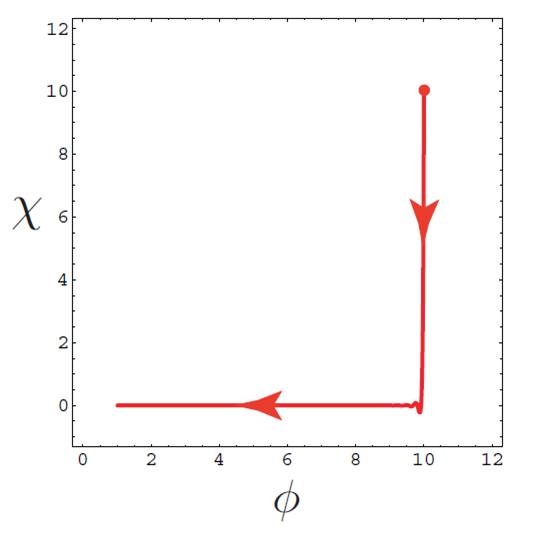
Figure 2: A background trajectory in double inflation model. Taken from Ref. [21].

5.1 Temporal slow-roll violation is not sufficient

First we consider double inflation model [54], which is a simple two-field model. The potential is given by

$$V(\phi,\chi)={1\over 2}m^{2}_{\phi}\phi^{2}+{1\over 2}m^{2}_{\chi}\chi^{2}.$$ (34)

There is no direct coupling between two fields, $\phi$ and $\chi$, except for gravitational one.

Here we follow the analysis of Ref. [21]. We show the background trajectory for $m_{\chi}/m_{\phi}=20$ in Fig. 2 taken from the same reference. Since the mass of $\chi$-field is much larger, the field moves rapidly in $\chi$-direction first. Arriving at around the minimum in $\chi$-direction, the slow roll conditions are violated and the field oscillates several times. This violation of slow-roll conditions at the intermediate step is possible when the mass ratio is large enough. Otherwise, the trajectory becomes just a smooth curve and slow roll conditions are not violated in the middle. One may expect that this temporal violation of slow roll produces large non-Gaussianity. However, this is not the case.

During the period when $\chi$-field is moving rapidly, $\phi$-field stays almost constant because the mass of $\phi$-field is small compared with the Hubble rate which is dominantly determined by the term $m^{2}_{\chi}\chi^{2}$ in the potential. Hence, the total e-folding number is simply given by the sum of e-foldings for two stages of inflation:

$$N=N^{(\phi)}+N^{(\chi)}\approx\phi_{*}^{2}+\chi_{*}^{2}.$$ (35)

Applying the formula (17), we find

$${6\over 5}f_{NL}={N_{i}N_{j}N^{ij}\over(N_{k}N^{k})^{2}}={2\over\phi_{*}^{2}+\chi_{*}^{2}}=O\left({1\over N}\right).$$ (36)

Hence, as in the usual slow-roll case, the non-Gaussianity is suppressed by the slow-roll parameter $\epsilon=O(1/N)$.

5.2 Simple hybrid inflation does not give large non-Gaussianity

As a second example, let’s consider hybrid inflation model [55] whose potential is given by

$$V(\phi,\chi)={\lambda\over 4}(\chi^{2}-v^{2})^{2}+{m^{2}\over 2}\phi^{2}+{g^{2}\over 2}\phi^{2}\chi^{2}.$$ (37)

Usually $\phi$ is the inflaton field and $\chi$ stays at $\chi=0$ during inflation. The effective mass of the $\chi$-field is a function of $\phi$ given by

$$m^{2}_{\chi}=-\lambda v^{2}+g^{2}\phi^{2},$$ (38)

assuming $\chi=0$. The mass of $\chi$-field changes its sign at some point, which we denote by $N=N_{c}$. Then, tachyonic instability in $\chi$-direction occurs, leading to the end of inflation.

To analyse the dynamics of $\chi$-field at this critical point analytically, we approximate the mass of $\chi$-field as

$$m^{2}_{\chi}=-\mu^{2}(N-N_{c}),$$ (39)

where $\mu^{2}$ is a parameter that depends on the choice of the model potential.

If $\mu^{2}\gtrsim H^{2}$, $\chi$-field is massive during $\phi$-field inflation. Thus, the fluctuation of $\chi$-field decays on large scales. If $\mu^{2}\lesssim H^{2}$, $\chi$ field can stay nearly massless during $\phi$-field inflation. In this case, the fluctuation of $\chi$-field may play an important role. As the mass scale of $\chi$ is small, we can apply the slow roll approximation to $\chi$-field, too. Then, we have

$$3H^{2}\partial_{N}\chi=\mu^{2}(N-N_{c})\chi.$$ (40)

This equation can be solved to obtain

$$\ln{\chi\over\chi_{*}}={\mu^{2}\over 6H^{2}}\left[(N-N_{c})^{2}-(N_{*}-N_{c})^{2}\right].$$ (41)

Applying the formula $(6/5)f_{NL}\approx N_{\chi\chi}/N_{\chi}^{2}$, which is valid when the fluctuation of $\chi$-field dominates, we have

$${6\over 5}f_{NL}\approx{\mu^{2}\over 3H^{2}}(N_{F}-N_{c}).$$ (42)

Since we are restricted to the case with $\mu^{2}\lesssim H^{2}$ and $N_{F}-N_{c}$ cannot be very large, $f_{NL}$ cannot be larger than 20 or so. If the fluctuations of $\phi$-field also contribute, which is usually required in order to produce almost scale invariant spectrum, the value of $f_{NL}$ becomes even smaller.

Furthermore, a more stringent constraint can be set by considering the following condition. If $\bar{\chi}(N_{c})\gtrsim H$ is not satisfied, fluctuations at the horizon scale modes at that time determine on which side the field rolls down. Then, the tachyonic instability does not keep the coherence of $\chi$-field on the super horizon scales, leading to the so-called spinodal decomposition. As a result, long wavelength fluctuation is, roughly speaking, completely erased. Hence, there is no chance to generate large non-Gaussianity originating from the fluctuation of $\chi$-field. The condition $\bar{\chi}(N_{c})\gtrsim H$ becomes

$${\mu^{2}\over 6H^{2}}(N_{F}-N_{c})^{2}\approx\ln{\chi_{F}\over\chi_{c}}\lesssim\ln{v\over H},$$ (43)

where we used the estimate $\chi_{F}\approx v$. Using this inequality, the above estimate for $f_{NL}$ (42) is bounded by

$${6\over 5}f_{NL}\lesssim{\mu\over H}\sqrt{{2\over 3}\ln{m_{pl}\over H}},$$ (44)

where we used $H^{2}=O(\lambda v^{4}/m^{2}_{pl})$ and $|m_{\chi}^{2}|_{\phi=0}=O(\lambda v^{2})>O(H)$. The latter condition is required to avoid topological inflation happens at $\phi=\chi=0$. The factor $\sqrt{{2\over 3}\ln{m_{p}l\over H}}$ is $\approx 7$ even if we reduce the energy scale of inflation $\sqrt{m_{pl}H}$ to TeV scale. Here, as $\mu^{2}\ll H^{2}$ is also required, we conclude that $f_{NL}$ cannot be much larger than unity.

5.3 Modular inflation

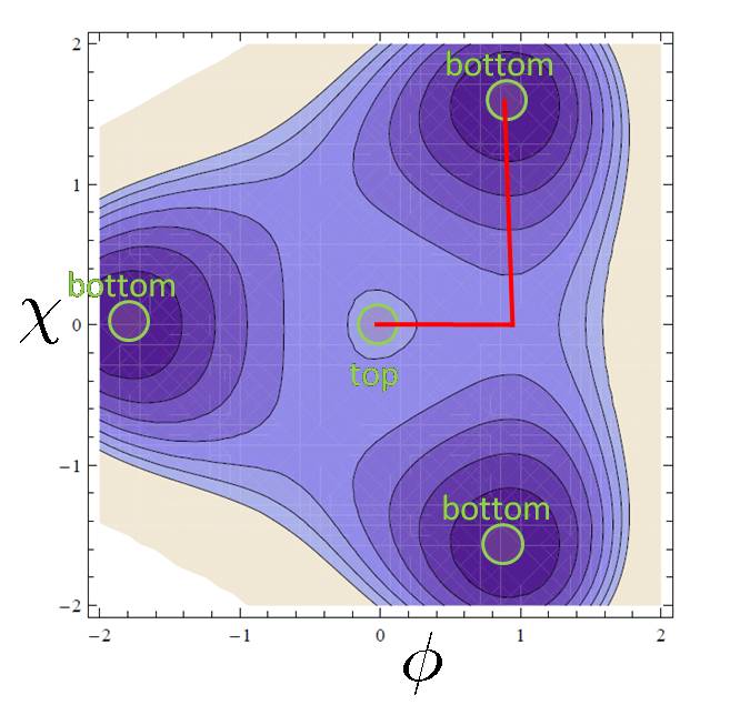
Figure 3: Contour plot of the potential of Kadota-Stewart model and a typical trajectory.

In the preceding subsection we have observed that large mass scale for the isocurvature modes is necessary to generate large non-Gaussianity. However, the mass squared should not be large positive at the early stage of inflation when the interesting scales exit the horizon. This requirement is not easily compromised unless we invent a very artificial form of potential just to produce large non-Gaussianity.

Here we given one rather natural model which satisfies our requirement. This is the model that was proposed by Kadota and Stewart [56]. The basic model potential takes the form

$$V=V_{0}-m_{\phi}^{2}|\Phi|^{2}+{1\over 3}m_{\Phi}^{2}(\Phi^{3}+h.c.)+m_{\Phi}^{2}|\Phi|^{4},$$ (45)

where again we set $m_{pl}=1$. $\Phi=(\phi+i\chi)/\sqrt{2}$ is a complex scalar field. This potential is modified near $\Phi=0$, the point with enhanced symmetry, due to loop correction of the Coleman-Weinberg type: $V_{loop}=-\beta m_{\phi}^{2}|\Phi|^{2}\ln\left|{\Phi/\Phi_{*}}\right|$. This correction produces ring-shaped maximum around $\Phi=0$, where topological inflation occurs. From the edges of the region of topological inflation, the field slowly rolls down the hill.

Contour plot of the potential is given in Fig. 3. We focus on the trajectories which pass near the saddle point as shown in the same figure with a red curve. In this model mass squared in the $\chi$-direction is negative from the beginning. However, since it is the direction of approximate $U(1)$ symmetry, the trajectories in any direction are almost equally preferred at this stage. As $\phi$ increases, the fluctuation in $\chi$-direction is enhanced by the ratio of $\phi$ compared with its initial value. After the direction of trajectory changes, this fluctuation in $\chi$-direction is transferred to the curvature perturbation. In this way the fluctuations in $\chi$-direction can rather easily dominate the final density perturbations. Then, the amplitude of fluctuations in $\chi$-direction stays almost constant near the ring-shaped top of potential, and therefore scale invariant spectrum is realised.

Near the saddle point, the equation in $\chi$-direction can be approximated by

$$3H^{2}\partial_{N}\chi=-m_{\chi}^{2}\chi,$$ (46)

with $m_{\chi}^{2}$ being the mass squared of $\chi$-field evaluated at the saddle point. Using the approximation $H^{2}=$constant, this equation can be solved to give

$$N={3H^{2}\over-m_{\chi}^{2}}\ln{\chi\over\chi_{*}},$$ (47)

where $\chi_{*}$ is the initial value of $\chi$. Applying the formula $(6/5)f_{NL}\approx N_{\chi\chi}/N_{\chi}^{2}$, we obtain

$${6\over 5}f_{NL}\approx{m_{\chi}^{2}\over 3H^{2}}.$$ (48)

This can be large if $m_{\chi}^{2}\gg H^{2}$. However, to achieve this by natural form of potential, the potential minima as well as the saddles points should be located close to the origin in Planck unit. Then, inflation does not occur except for the top of the potential or near the saddle points. To sustain a sufficiently large e-folding number, inflation in these specific regions should last long. However, this is not allowed. If inflation lasts long near the top of the potential, which is ring-shaped, the motion in the radial direction becomes very slow. As a result, the amplitude of curvature perturbation originating from the fluctuation in $\phi$ direction dominates. For inflation to last long near the saddle point, the trajectory should pass very close to the saddle point. However, in such cases significant fraction of the universe will fall into the other side of the saddle point. As a result domain walls are formed, which leads to the problematic domain wall dominated universe.

Even if we can avoid the domain wall formation (by considering models with higher symmetry), it is not easy to construct models which explain the naturalness of such a special trajectory. The probability distribution of the universes with different values of $\chi_{*}$ will be affected by the volume expansion factor during inflation, which is proportional to $e^{3N}$. If ${3H^{2}/|m_{\chi}^{2}|}$ is small as is requested for large non-Gaussianity, $\chi_{*}$ must be extremely small to gain a large e-folding there. Then, the probability of having such a small value of $\chi_{*}$ is extremely small. As long as we consider models which realize sufficiently large e-foldings for the natural choice of the fiducial value of $\chi_{*}$, $f_{NL}$ will not largely exceed unity. Further variation of this model is possible by introducing loop correction at around the saddle points, but the final conclusion does not change much. We will report detailed analysis about this model in our future publication.

6 Conclusion

Multi-field inflation generates entropy perturbation as well as the adiabatic one. This entropy perturbation in general affects the evolution of the curvature perturbation even after the horizon crossing. Possible mechanisms of production of non-Gaussianity in the super-horizon regime can be classified into two cases. One is the production of non-Gaussianity during inflation and the other is that at the end of or after inflation. Although we could not give a general proof, it seems very difficult to produce large non-Gaussianity during inflation as far as we consider potential without fine-tuning, although there are several claims that suggest it possible .

Here are several subtle issues. In this paper we claimed it difficult to construct a natural model in which large non-Gaussianity originating from the non-linear evolution is produced before inflation terminates. By contrast, generation of large non-Gaussianity at the end of or after inflation is rather easy. However, it may not be so trivial in general to identify when non-Guassianity is generated. We gave an example of double inflation in § 5.1. Although we did not mention it in the text, in this model the non-linear parameter $f_{NL}$ as a function of $t_{F}$ becomes very large temporally when the background trajectory changes its direction, but this large $f_{NL}$ does not persist long. This means that the time dependence of $f_{NL}$ is not always appropriate to read when non-Gaussianity is mainly generated.

Another important point to note is the limitation of neglecting small scale perturbations. The small scale perturbations often become important for the field components that become massive during inflation. A typical example is the hybrid inflation model discussed in § 5.2. To take into account the effect of small scale perturbations, $\delta N$ formalism based on the background evolution for spatially homogeneous spacetime is not sufficient. We need to extend $\delta N$ formalism incorporating collective variables that characterise statistical state such as the averaged magnitude of small scale fluctuation.

Finally we should mention the naturalness of the initial conditions. It might be possible to obtain large non-Gaussianity by tuning the initial conditions, but it will not be realised in reality if they are extremely fine-tuned. As an example, we discussed Kadota-Stewart model in § 5.3. However, once we start to discuss the likeliness of the chosen initial conditions, the long-standing measure problem arises. At the moment we are very far from a conclusive answer on this issue.

References

References

- [1] E. Komatsu et al., arXiv:1001.4538.
- [2] e.g., V. F. Mukhanov, H. A. Feldman and R. H. Brandenberger, Phys. Rept. 215, 203 (1992), Part 2.
- [3] A. A. Starobinsky, JETP Lett. 42, 152 (1985) [Pisma Zh. Eksp. Teor. Fiz. 42, 124 (1985)].
- [4] D. S. Salopek and J. R. Bond, Phys. Rev. D 42, 3936 (1990).
- [5] M. Sasaki and E. D. Stewart, Prog. Theor. Phys. 95, 71 (1996) [arXiv:astro-ph/9507001].
- [6] M. Sasaki and T. Tanaka, Prog. Theor. Phys. 99, 763 (1998) [arXiv:gr-qc/9801017].
- [7] D. H. Lyth, K. A. Malik and M. Sasaki, JCAP 0505, 004 (2005) [arXiv:astro-ph/0411220].
- [8] D. H. Lyth and Y. Rodriguez, Phys. Rev. Lett. 95, 121302 (2005) [arXiv:astro-ph/0504045].
- [9] N. Mandolesi et al., arXiv:1001.2657.
- [10] D. Baumann et al. [CMBPol Study Team Collaboration], AIP Conf. Proc. 1141, 10 (2009) [arXiv:0811.3919].
- [11] http://quiet.uchicago.edu/
- [12] E. Komatsu and D. N. Spergel, Phys. Rev. D 63, 063002 (2001) [arXiv:astro-ph/0005036].
- [13] N. Bartolo, E. Komatsu, S. Matarrese and A. Riotto, Phys. Rept. 402, 103 (2004) [arXiv:astro-ph/0406398].
- [14] J. M. Maldacena, JHEP 0305, 013 (2003) [arXiv:astro-ph/0210603].
- [15] D. Seery and J. E. Lidsey, JCAP 0506, 003 (2005) [arXiv:astro-ph/0503692].
- [16] D. Seery, J. E. Lidsey and M. S. Sloth, JCAP 0701, 027 (2007) [arXiv:astro-ph/0610210].
- [17] D. Seery and J. E. Lidsey, JCAP 0509, 011 (2005) [arXiv:astro-ph/0506056].
- [18] K. A. Malik and D. Wands, Class. Quant. Grav. 21, L65 (2004) [arXiv:astro-ph/0307055].
- [19] K. A. Malik, JCAP 0511, 005 (2005) [arXiv:astro-ph/0506532].
- [20] S. Yokoyama, T. Suyama and T. Tanaka, JCAP 0707, 013 (2007) [arXiv:0705.3178].
- [21] S. Yokoyama, T. Suyama and T. Tanaka, Phys. Rev. D 77, 083511 (2008) [arXiv:0711.2920].
- [22] C. T. Byrnes, M. Sasaki and D. Wands, Phys. Rev. D 74, 123519 (2006) [arXiv:astro-ph/0611075].
- [23] C. T. Byrnes, K. Koyama, M. Sasaki and D. Wands, JCAP 0711, 027 (2007) [arXiv:0705.4096].
- [24] S. Yokoyama, T. Suyama and T. Tanaka, JCAP 0902, 012 (2009) [arXiv:0810.3053].
- [25] P. Creminelli, JCAP 0310, 003 (2003) [arXiv:astro-ph/0306122].
- [26] M. Alishahiha, E. Silverstein and D. Tong, Phys. Rev. D 70, 123505 (2004) [arXiv:hep-th/0404084].
- [27] K. Koyama, arXiv:1002.0600.
- [28] L. Alabidi, JCAP 0610, 015 (2006) [arXiv:astro-ph/0604611].
- [29] K. A. Malik and D. H. Lyth, JCAP 0609, 008 (2006) [arXiv:astro-ph/0604387].
- [30] M. Sasaki, J. Valiviita and D. Wands, Phys. Rev. D 74, 103003 (2006) [arXiv:astro-ph/0607627].
- [31] G. Dvali, A. Gruzinov and M. Zaldarriaga, Phys. Rev. D 69, 023505 (2004) [arXiv:astro-ph/0303591].
- [32] F. Bernardeau and J. P. Uzan, Phys. Rev. D 66, 103506 (2002) [arXiv:hep-ph/0207295].
- [33] F. Bernardeau and J. P. Uzan, Phys. Rev. D 67, 121301 (2003) [arXiv:astro-ph/0209330].
- [34] D. H. Lyth, JCAP 0511, 006 (2005) [arXiv:astro-ph/0510443].
- [35] M. P. Salem, Phys. Rev. D 72, 123516 (2005) [arXiv:astro-ph/0511146].
- [36] D. Seery and J. E. Lidsey, JCAP 0701, 008 (2007) [arXiv:astro-ph/0611034].
- [37] L. Alabidi and D. Lyth, JCAP 0608, 006 (2006) [arXiv:astro-ph/0604569].
- [38] C. T. Byrnes and G. Tasinato, “Non-Gaussianity beyond slow roll in multi-field inflation,” JCAP 0908 (2009) 016 [arXiv:0906.0767].
- [39] C. T. Byrnes, K. Y. Choi and L. M. H. Hall, JCAP 0810, 008 (2008) [arXiv:0807.1101].
- [40] C. T. Byrnes and K. Y. Choi, arXiv:1002.3110.
- [41] H.R.S. Cogollo, Y. Rodriguez and C.A. Valenzuela-Toledo, JCAP 0808, 029 (2008) [arXiv:0806.1546].
- [42] Y. Rodriguez and C.A. Valenzuela-Toledo: Phys. Rev. D 81, 023531 (2010) [arXiv:0811.4092].
- [43] K. Enqvist, A. Jokinen, A. Mazumdar, T. Multamaki and A. Vaihkonen, Phys. Rev. Lett. 94, 161301 (2005) [arXiv:astro-ph/0411394].
- [44] A. Jokinen and A. Mazumdar, JCAP 0604, 003 (2006) [arXiv:astro-ph/0512368].
- [45] A. Chambers and A. Rajantie, Phys. Rev. Lett. 100, 041302 (2008) [Erratum-ibid. 101, 149903 (2008)] [arXiv:0710.4133].
- [46] A. Chambers and A. Rajantie, JCAP 0808, 002 (2008) [arXiv:0805.4795].
- [47] N. Barnaby and J. M. Cline, Phys. Rev. D 73, 106012 (2006) [arXiv:astro-ph/0601481].
- [48] D. Mulryne, D. Seery and D. Wesley, arXiv:0911.3550.
- [49] T. Tanaka and B. Bassett, published in the proceedings of 12th Workshop on General Relativity and Gravitation, arXiv:astro-ph/0302544.
- [50] T. Suyama and S. Yokoyama, Class. Quant. Grav. 24, 1615 (2007) [arXiv:astro-ph/0606228].
- [51] T. Moroi and T. Takahashi, Phys. Lett. B 522, 215 (2001) [Erratum-ibid. B 539, 303 (2002)] [arXiv:hep-ph/0110096].
- [52] D. H. Lyth and D. Wands, Phys. Lett. B 524, 5 (2002) [arXiv:hep-ph/0110002].
- [53] E. D. Stewart, Phys. Rev. D 65, 103508 (2002) [arXiv:astro-ph/0110322].
- [54] J. Silk and M. S. Turner, Phys. Rev. D 35, 419 (1987).
- [55] A. D. Linde, Phys. Rev. D 49, 748 (1994) [arXiv:astro-ph/9307002].
- [56] K. Kadota and E. D. Stewart, JHEP 0307, 013 (2003) [arXiv:hep-ph/0304127].