Transport properties of the fluid produced at RHIC

Abstract

It is by now well known that the relativistic heavy-ion collisions at RHIC, BNL have produced a strongly interacting fluid with remarkable properties, among them the lowest ever observed ratio of the coefficient of shear viscosity to entropy density. Arguments based on ideas from the String Theory, in particular the AdS/CFT correspondence, led to the conjecture — now known to be violated — that there is an absolute lower limit $1/4\pi$ on the value of this ratio. Causal viscous hydrodynamics calculations together with the RHIC data have put an upper limit on this ratio, a small multiple of $1/4\pi$, in the relevant temperature regime. Less well-determined is the ratio of the coefficient of bulk viscosity to entropy density. These transport coefficients have also been studied nonperturbatively in the lattice QCD framework, and perturbatively in the limit of high-temperature QCD. Another interesting transport coefficient is the coefficient of diffusion which is also being studied in this context. I review some of these recent developments and then discuss the opportunities presented by the anticipated LHC data, for the general nuclear physics audience.

1. Introduction

Transport coefficients of the QCD matter are of fundamental importance not only because they represent an important aspect of QCD, but also because they can be calculated from first principles. Trying to extract these coefficients reliably from experimental data and evaluating them in various theoretical approaches is a very active area of research today.

This review is addressed to the general Nuclear Physics audience, a majority of whom do not work in the area of relativistic heavy-ion collisions, but have probably heard the claim that the RHIC experiments have produced the most perfect fluid ever observed. Before I explain the meaning of this claim and present the experimental evidence for it, a few introductory remarks are in order. It may be recalled that the phase diagram (pressure vs temperature) of the most familiar liquid, namely water is known for long with good accuracy. In particular, the coordinates of the triple point and the critical point are known to several significant places, and the various phase co-existence lines are well-determined. In contrast, the phase diagram of the strongly-interacting matter or the QCD phase diagram (temperature vs the net baryon number density or equivalently the baryon number chemical potential) is known only schematically from the experimentalist’s point of view. Indeed, it is not even known with certainty what are the various phases that occur at high densities.

The big idea is to map out quantitatively the QCD phase diagram with the relativistic heavy-ion collisions as an experimental tool. Such experiments have been performed at SPS (CERN), are being performed at RHIC (BNL), and will soon be performed at LHC (CERN), at successively higher energies: up to $\sqrt{s}_{NN}=$ 19, 200 and 5400 GeV, at the above three facilities, respectively. It is also necessary to systematically scan the energy range up to 200 GeV in order to study the QCD matter at high baryon number density and to locate the critical point and the phase transition line predicted by some theories. This is being done at RHIC and plans are afoot to do it at FAIR (GSI) and NICA (JINR).

In nonrelativistic fluid dynamics, the kinematic viscosity ($\nu$) is defined as $\nu=\eta/\rho$ where $\eta$ is the coefficient of shear viscosity or the dynamic viscosity and $\rho$ is the density of the fluid. It allows us to compare the viscosities of fluids with different densities. (Interestingly, under standard conditions, water has a lower $\nu$ than air, although its $\eta$ is higher.) The dimensionless ratio $\eta/s$ serves as the relativistic analog of the kinematic viscosity, $s$ being the entropy density. (The dimensionless ratio $\eta/n$ where $n$ is the number density is of no use here because $n$ is ill-defined in relativistic heavy-ion collisions.)

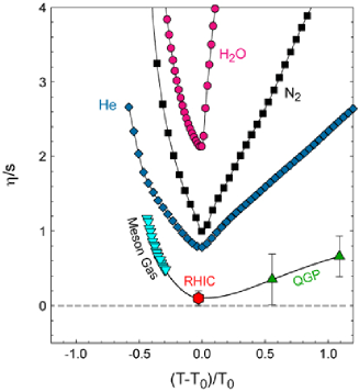
Figure  1.: Comparison of different fluids with each other. See the text for details. The lines are drawn to guide the eye. Figure from Ref.  [?].

Figure 1 shows $\eta/s$ as a function of $(T-T_{0})/T_{0}$ where $T$ is the temperature and $T_{0}$ the critical temperature, for various fluids, namely water, nitrogen, helium and the QCD matter. The upper three curves, drawn at the respective critical pressures, exhibit a cusp at $T_{0}$. The liquid and gaseous phases behave differently because the momentum transport mechanisms are different in the two cases; see, e.g.,  [?]. The points labelled Meson Gas have large ($\sim 50$ %) errors and are obtained from chiral perturbation theory. The points labelled QGP are from lattice QCD simulations of  [?]. The point labelled RHIC is discussed below. This comparison of various fluids explains the statement that the RHIC fluid is the most perfect fluid ever observed.

The point labelled RHIC in Fig. 1 was obtained by matching the elliptic flow data at RHIC with the results of viscous hydrodynamic calculations: Consider a non-central collision of two identical spherical nuclei as shown in Fig. 2. The nuclei travel parallel to the $z$ axis, $xy$ plane is the azimuthal or transverse plane and $xz$ plane is called the reaction plane. The overlap zone is shown as the shaded area in the figure. In an ultrarelativistic collision, the nucleons in the non-overlapping zones continue to travel more or less along their pre-collision trajectories, leaving behind the almond-shaped overlap zone. The interesting observables are governed mostly by the overlap zone which has a very high initial energy density. The spatial anisotropy of the overlap zone ensures anisotropic pressure gradients in the $xy$ plane. This leads to a final state characterized by momentum anisotropy and anisotropic distribution of particles in the $xy$ plane.

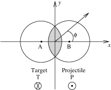
Figure  2.: Non-central collision of two nuclei.

The triple differential invariant distribution of particles emitted in the final state is given by

$\displaystyle E\frac{d^{3}N}{d^{3}p}=\frac{d^{3}N}{p_{T}dp_{T}dyd\phi}=\frac{d^{2}N}{p_{T}dp_{T}dy}\frac{1}{2\pi}\left[1+\sum_{1}^{\infty}2v_{n}\cos(n\phi)\right],$

where $p_{T}$ is the transverse momentum, $y$ the rapidity and $\phi$ the azimuthal angle of an emitted particle. The azimuthal distribution is Fourier-decomposed, and the leading coefficients $v_{1}$ and $v_{2}$ are called the directed and elliptic flow, respectively. They provide a measure of the anisotropy of the flow in the transverse plane, mentioned above. The importance of $v_{2}$ lies in the fact that it is a measure of pressure at early times and hence the measure of thermalization of the quark-gluon matter produced in heavy-ion collisions.

Hydrodynamics is an effective theory that describes the slow, long-wavelength motion of a fluid close to equilibrium. It is a powerful technique because given the initial conditions and only the equation of state (EoS) of the matter, it predicts the space-time evolution of the fluid. Its limitation is that it is applicable at or near (local) thermodynamic equilibrium only. Hydrodynamics plays a central role in modeling relativistic heavy-ion collisions. State-of-the-art calculations for the RHIC data are based on the relativistic causal dissipative hydrodynamics. However, the initial calculations were done in the ideal ($\eta/s=0$) hydrodynamics framework. As an example, see Fig. 3. The broad agreement between the data and these initial calculations, in particular the mass ordering of $v_{2}(p_{T})$, led to the claim of formation of an ideal fluid at RHIC.

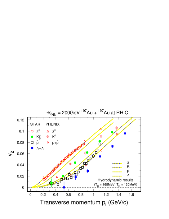
Figure  3.: Success of ideal hydrodynamics: Minimum-bias elliptic flow data compared with ideal hydrodynamics calculations of Huovinen. Figure from Ref.  [?].

2. Transport Coefficients

Consider a fluid in equilibrium. If it is perturbed so that the density is no longer uniform, it responds by setting up currents which tend to restore the equilibrium. In the linear response theory, the current or flux is proportional to the force which is negative of the gradient of the density: $\rho{\bf u}=-D\nabla\rho$. The constant of proportionality ($D$) is called the coefficient of diffusion. Other familiar examples are Ohm’s law ${\bf J}=\sigma{\bf E}=-\sigma\nabla\phi$, Fourier’s law of heat conduction ${\bf Q}=-\kappa\nabla T$, etc. A slightly more complicated example involves the transport of momentum in response to velocity gradients in an anisotropic medium, the constant of proportionality being the shear viscosity tensor. Such equations are called constitutive equations because they express physical properties of the material concerned. They relate the fluxes with the forces, the constants of proportionality being the transport coefficients.

In addition to the variables such as the hydrodynamic four-velocity, pressure, energy density, conserved-number density, etc., hydrodynamics equations also contain transport coefficients (shear and bulk viscosities, thermal conductivity, relaxation times, etc.). These are external parameters which can be calculated in a variety of ways (see Table 1) and fed into the hydrodynamics equations.

Table 1.: Various ways to calculate transport coefficients for relativistic fluids

Weak-coupling regime	Kinetic Theory	Boltzmann Equation
	Linear-Response Theory	Kubo Formula
	N=4 Supersymmetric Yang-Mills Theory
Strong-coupling regime	Lattice Gauge Theory	Kubo Formula
	N=4 Supersymmetric Yang-Mills Theory

2.1 Transport coefficients from high-temperature QCD

High-temperature QCD assumes $T\gg\Lambda_{QCD}$. This is a weak-coupling regime and the shear ($\eta$) and bulk ($\zeta$) viscosities can be calculated in the kinetic theory  [?], [?], [?]:

$\displaystyle\eta\sim\frac{T^{3}}{\alpha_{s}^{2}\ln\alpha_{s}^{-1}},~{}~{}~{}\zeta\sim\frac{\alpha_{s}^{2}T^{3}}{\ln\alpha_{s}^{-1}}.$

It is clear that as the temperature $T$ rises, $\eta/T^{3}$ increases while $\zeta/T^{3}$ decreases, and the ratio $\zeta/\eta\sim\alpha_{s}^{4}$ decreases. Note that the bulk viscosity vanishes for any conformal field theory, and QCD becomes conformal in the limit of high $T$. On the other hand, when $T\sim 200$ MeV, QCD is far from weakly coupled and the above results can provide only a rough estimate of $\eta$ and $\zeta$.

2.2 Transport coefficients from string theory

Like ordinary fluids black holes too are thermal systems having notions of temperature and entropy. An object falling on the surface of a fluid in equilibrium generates disturbance which dies down due to dissipative nature of the fluid. Similarly, the black hole horizon gets deformed when an object falls on it. However, it soon recovers its equilibrium shape. Thus the notion of “viscosity” is applicable to a black hole as well, and the connection between hydrodynamics and black-hole physics does not seem very far-fetched.

Anti-deSitter/conformal field theory (AdS/CFT) correspondence refers to the equivalence or duality between string theory defined on a certain AdS space and a CFT defined on its boundary. It allows the calculation of properties of a strongly-coupled CFT in terms of those of a weakly-coupled string theory. For an elementary introduction to these ideas, see  [?].

Ordinary quantum mechanics rules out vanishing $\eta/s$ for weakly coupled theories, i.e., for theories with well-defined quasiparticles  [?]. Kovtun et al.  [?], using string theory methods, showed that $\eta/s=1/4\pi$, for a large class of strongly interacting quantum field theories whose dual description involves black holes in the Anti-deSitter (AdS) space. The value $1/4\pi$ was conjectured to be its absolute lower bound (KSS bound) for all substances. However, it has recently been realized that the KSS bound is violated for certain conformal field theories (CFT)  [?], [?].

Of course, applying above ideas to the fluid produced at RHIC is speculative: QCD near the deconfinement transition temperature is not a CFT, and its gravity dual (if it exists) is not known.

2.3 Transport coefficients from lattice QCD

Figure 4 shows the results of a quenched QCD (no dynamical quarks or $m_{q}\rightarrow\infty$) calculation of $\eta/s$ from Ref.  [?] in comparison with the high-$T$ QCD results quoted in subsection 2.1 and the KSS bound mentioned in the previous subsection. However, these initial results have now been superseded by more recent results described next.

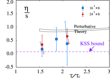
Figure  4.: First lattice QCD results on $\eta/s$. Figure from Ref.  [?].

Recently Meyer has calculated both $\eta/s$ and $\zeta/s$ on the lattice, with higher statistical accuracy and a more efficient algorithm, assuming SU(3) gluodynamics  [?], [?]. He gets

$\displaystyle\eta/s=\left\{\begin{array}[]{l@{~~~}l}0.134(33)\hfil~{}~{}~{}&(T=1.65T_{c})\\ 0.102(56)\hfil~{}~{}~{}&(T=1.24T_{c}),\end{array}\right.$

where the errors contain an estimate of the systematic uncertainty. This is consistent with the KSS bound. Further,

$\displaystyle\zeta/s=\left\{\begin{array}[]{l@{~~~}l}0.008(7)\Big{[}\begin{array}[]{c}\scriptstyle{0.15}\\ \scriptstyle{0}\end{array}\ \Big{]}\hfil~{}~{}~{}&(T=1.65T_{c})\\ 0.065(17)\Big{[}\begin{array}[]{c}\scriptstyle{0.37}\\ \scriptstyle{0.01}\end{array}\Big{]}\hfil~{}~{}~{}&(T=1.24T_{c}),\end{array}\right.$

$\displaystyle\zeta/s=0.73(3)\Big{[}\begin{array}[]{c}\scriptstyle{2.0}\\ \scriptstyle{0.5}\end{array}\Big{]}\qquad(T=1.02T_{c}),$

where the statistical error is given and the square bracket specifies conservative upper and lower bounds. Note the sharp rise in $\zeta/s$ just above $T_{c}$. Similar dramatic rise was seen in the results presented in  [?]; see Figure 5.

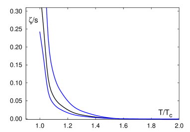
Figure  5.: Bulk viscosity vs temperature. The three curves (top to bottom) correspond to $\omega_{0}(T)=0.5,1,1.5$ GeV respectively, where $\omega_{0}(T)$ is a scale at which the perturbation theory becomes valid. The three curves reflect the uncertainty in the determination of this scale parameter. Figure from Ref.  [?]. See, however, the discussion in the text.

They extracted the bulk viscosity in the presence of light quarks by combining low-energy theorems with lattice data on the QCD EoS. However, it is now realized that a determination of $\zeta$ from correlation functions of the energy-momentum tensor is more subtle. Shortcomings of this calculation have been pointed out in  [?]. If the sharp rise of $\zeta/s$ just above $T_{c}$ is confirmed, it would imply that the QGP is not a perfect fluid near $T_{c}$!

For a review of the progress made in extracting transport properties of the gluonic plasma from lattice simulations, see  [?].

2.4 Transport coefficients extracted from RHIC data

Here the basic idea is that the shear viscosity reduces the elliptic flow: $v_{2}({\rm viscous~{}fluid})<v_{2}({\rm ideal~{}fluid})$. This is easy to understand: recall that $v_{2}$ is a measure of the flow anisotropy in the azimuthal plane. Viscosity is the result of a frictional force. Frictional force being proportional to the flow velocity has a relatively stronger effect on fast-moving particles emerging in the reaction plane. This reduces the anisotropy and hence $v_{2}$.

Thus if one has a good control on $v_{2}({\rm ideal~{}fluid})$, one can adjust $\eta/s$ to fit the data on $v_{2}$, and thus extract $\eta/s$. This has been done by several groups  [?],  [?],  [?],  [?], [?], [?],  [?]. Results of  [?] are shown in Fig. 6. The Glauber and colour-glass-condensate (CGC) initial conditions for hydrodynamic evolution yield $\eta/s\simeq 0.08$ and $\simeq 0.16$ respectively, showing the sensitivity of the extracted $\eta/s$ to the initial conditions.

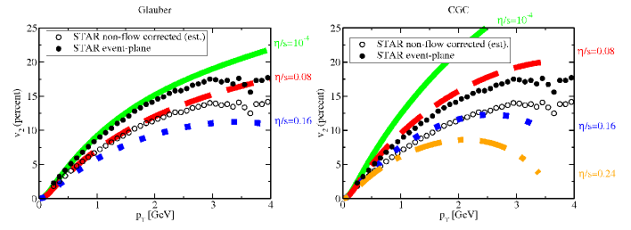
Figure  6.: Minimum-bias elliptic flow data for charged hadrons in 200 GeV Au-Au collisions; only statistical errors are shown. Line thickness is an estimate of the accumulated numerical error. Figure from Ref.  [?].

3. Diffusion

Transport of heat occurs by diffusion (Fourier’s law) as well as by propagating waves (Maxwell-Cattaneo law). The latter mechanism underlies the well-known phenomenon of second sound in superfluid helium (Table 2). Similarly the transport of momentum too occurs by diffusion (Navier-Stokes equation) or by propagating waves. These are the transverse or shear waves, different from the more familiar longitudinal or compressional waves. For a detailed discussion see  [?].

Table 2.: Various transport phenomena

Transport of	By diffusion	By propagating waves	Experimental situation
Heat	Fourier’s law	Maxwell-Cattaneo law	Second sound in superfluid He
Momentum	Navier-Stokes eq.	Maxwell-Cattaneo law	Propagating shear waves
Conserved no.	Fick’s law	Kelly’s law	RHIC?
e.g., B, Q, S

We recently studied the transport of a conserved number such as the net baryon number ($B$), charge ($Q$), or strangeness ($S$) conserved in strong interactions, in the acausal and causal, or the first- and second-order theories of relativistic diffusion  [?]. We found that Fick’s diffusion smooths out gradients in the number density monotonically. In contrast, in Kelly’s theory the gradients may be transiently amplified, i.e., the density profile may stiffen at intermediate times; see Fig. 7. We proposed experimental observables and argued that the RHIC data can potentially distinguish between the above two mechanisms. If the second-order theory of diffusion is ruled out by the data, one gets a handle on the relaxation time and hence on thermalization.

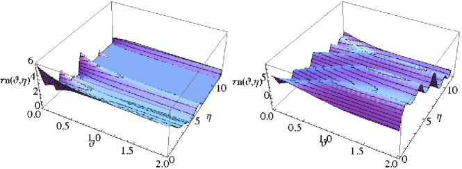
Figure  7.: Conserved number density profile as a function of time and space-time rapidity in the Fick (left) and Kelly (right) theories of diffusion. Figure from Ref.  [?].

4. Viscosity in Ordinary Finite Nuclei

This review is about the transport properties of the fluid produced at RHIC. But it is pertinent to ask what do we know about the transport coefficients of the matter in an ordinary finite nucleus at low temperatures. Hydrodynamic models have a long history in Nuclear Physics — recall the success of the liquid drop model. The coefficient of shear viscosity of a finite nucleus can be obtained from (i) analysis of the widths of giant resonances within the hydrodynamic model, (ii) the process of fission studied within the liquid drop model, and (iii) kinetic theory. This has been discussed recently in  [?]. Using entropy density for a free Fermi gas or for noninteracting nucleons in a Woods-Saxon potential, they obtained values of $\eta/s$ larger than but not drastically different from those for the RHIC fluid.

5. What about LHC?

It is clear from Table 3 that at LHC we would need $\eta/s$ and $\zeta/s$ up to $T\sim 4T_{c}$. Some preliminary lattice results are now available, but for the SU(3) pure gauge theory (i.e., quarkless QCD)  [?]. For a careful extraction of $\eta/s$ and $\zeta/s$ from LHC (and RHIC) data, we need to incorporate the $T$-dependence of these transport coefficients in hydrodynamic calculations, among other refinements of these calculations; see the next section.

Table 3.: Comparison of central Au-Au collisions at RHIC and central Pb-Pb collisions at LHC

	RHIC (Au-Au)	LHC (Pb-Pb)
$\sqrt{s}_{NN}$	200 GeV	5.5 TeV
Initial temperature	$\sim$2Tc	$\sim$4Tc
Initial energy density	$\sim 5$ GeV/fm3	15-60 GeV/fm3
Lifetime	$\sim 10$ fm/c	$>$ 10 fm/c

6. Take-Home Message

• Elliptic flow at RHIC has put a robust upper limit on the value of $\eta/s$ of the RHIC fluid: $\eta/s\mathrel{\hbox to0.0pt{\lower 4.0pt\hbox{\hskip 1.0pt$\sim$}\hss}\raise 1.0pt\hbox{$<$}}5/(4\pi)$. This is the average value in the relevant temperature region.

• Uncertainties associated with the initial conditions, EoS, bulk viscosity, hadronic stage, freezeout procedure, different versions of the second-order hydrodynamic equations prevent a more precise determination of $\eta/s$. See Ref.  [?] for a detailed discussion.

• The bulk viscosity is not yet well-determined in the deconfinement transition region.

• Analysis of the RHIC data, which might throw light on the coefficient of diffusion, is awaited.

Acknowledgments

I thank Sourendu Gupta and Jean-Yves Ollitrault for a critical reading of the manuscript.

REFERENCES

- [1] R. A. Lacey et al., Phys. Rev. Lett. 98, 092301 (2007)
- [2] L. P. Csernai, J. I. Kapusta and L. D. McLerran, Phys. Rev. Lett. 97, 152303 (2006)
- [3] A. Nakamura and S. Sakai, Phys. Rev. Lett. 94, 072305 (2005)
- [4] M. D. Oldenburg [STAR Collaboration], J. Phys. G 31, S437 (2005)
- [5] P. Arnold, G. D. Moore and L. G. Yaffe, JHEP 0011, 001 (2000)
- [6] P. Arnold, G. D. Moore and L. G. Yaffe, JHEP 0305, 051 (2003)
- [7] P. Arnold, C. Dogan and G. D. Moore, Phys. Rev. D 74, 085021 (2006)
- [8] M. Natsuume, arXiv:hep-ph/0701201
- [9] P. Danielewicz and M. Gyulassy, Phys. Rev. D 31, 53 (1985)
- [10] P. Kovtun, D. T. Son and A. O. Starinets, Phys. Rev. Lett. 94, 111601 (2005)
- [11] A. Buchel, R. C. Myers and A. Sinha, JHEP 0903, 084 (2009)
- [12] M. Brigante, H. Liu, R. C. Myers, S. Shenker and S. Yaida, Phys. Rev. Lett. 100, 191601 (2008)
- [13] H. B. Meyer, Phys. Rev. D 76, 101701 (2007)
- [14] H. B. Meyer, Phys. Rev. Lett. 100, 162001 (2008)
- [15] F. Karsch, D. Kharzeev and K. Tuchin, Phys. Lett. B 663, 217 (2008)
- [16] K. Huebner, F. Karsch and C. Pica, Phys. Rev. D 78, 094501 (2008)
- [17] H. B. Meyer, Nucl. Phys. A 830, 641C (2009)
- [18] R. J. Fries, B. Muller and A. Schafer, Phys. Rev. C 78, 034913 (2008)
- [19] P. Romatschke and U. Romatschke, Phys. Rev. Lett. 99, 172301 (2007)
- [20] M. Luzum and P. Romatschke, Phys. Rev. C 78, 034915 (2008) [Erratum-ibid. C 79, 039903 (2009)]
- [21] H. Song and U. W. Heinz, Phys. Rev. C 77, 064901 (2008)
- [22] K. Dusling and D. Teaney, Phys. Rev. C 77, 034905 (2008)
- [23] D. Molnar and P. Huovinen, J. Phys. G 35, 104125 (2008)
- [24] A. K. Chaudhuri, Phys. Lett. B 681, 418 (2009)
- [25] P. Romatschke, arXiv:0902.3663 [hep-ph]
- [26] R. S. Bhalerao and S. Gupta, Phys. Rev. C 79, 064901 (2009)
- [27] N. Auerbach and S. Shlomo, Phys. Rev. Lett. 103, 172501 (2009)
- [28] U. W. Heinz, J. S. Moreland and H. Song, Phys. Rev. C 80, 061901 (2009)