Berry-Phase induced Heat Pumping and its Impact on the Fluctuation Theorem

Abstract

Applying adiabatic, cyclic two parameter modulations we investigate quantum heat transfer across an anharmonic molecular junction contacted with two heat baths. We demonstrate that the pumped heat typically exhibits a Berry phase effect in providing an additional geometric contribution to heat flux. Remarkably, a robust fractional quantized geometric phonon response is identified as well. The presence of this geometric phase contribution in turn causes a breakdown of the fluctuation theorem of the Gallavotti-Cohen type for quantum heat transfer. This can be restored only if (i) the geometric phase contribution vanishes and if (ii) the cyclic protocol preserves the detailed balance symmetry.

Understanding and controlling of heat transfer due to phonons occurring in low dimensional nanoscale systems is both of prime and practical importance WL08 . Pioneering experimental works carried out recently, such as nanotube thermal rectifier exp_diode , nanotube phonon waveguide waveguide has spawn phononics, i.e. the science and engineering of phonons WL08 , as an emerging new scientific discipline where heat flow can be manipulated as flexibly as electronic current. Although the nonlinear (anharmonic) interaction has been demonstrated as a crucial component Li06 ; Wu09 in various functional thermal devices, the heat control has heretofore typically been achieved by applying a temperature bias, for which in accordance with the second law of thermodynamics – heat flows from “hot” to “cold” spontaneously.

Recent studies show that spontaneous, rare fluctuations of anomalous heat transfer may occur RMP , thus being seemingly in apparent violation with the second law. Clearly, however, no violation of the second law occurs on average. The typical measure of such violations is the (small) probability for such anomalous events as they emerge from a heat exchange fluctuation theorem (FT) RMP ; Jarzynski04 ; Saito07 ; Talkner09 . The FT for (nonequilibrium) entropy production Evans1993 ; GC1995 and heat flux Jarzynski04 ; Saito07 describes that the distribution, $P_{\tau}(Q)$, of the heat $Q$ transferred from the left ($L$) bath at temperature $T_{L}$ to the right ($R$) bath at $T_{R}$ over a long time interval $\tau$, obeys the relation: $\lim\limits_{\tau\rightarrow\infty}{\tau}^{-1}\ln[{P_{\tau}(Q)}/{P_{\tau}(-Q)}]=Q(\beta_{R}-\beta_{L})/\tau,$ where $\beta_{L,R}=1/k_{B}T_{L,R}$. This FT thus shows explicitly that heat can transfer spontaneously from “cold” to “hot” with finite, although typically with very small probability. In particular, Ref. Saito07 demonstrates this FT in the quantum case for heat transfer across a quantum harmonic chain coupled with thermal reservoirs. A particular challenge that arises is then whether this quantum Gallavotti-Cohen type FT remains valid also in the nonlinear quantum regime beyond the quantum harmonic chain limit, and, more generally, whether such a heat-flux FT still can be formulated in presence of cyclic time-dependent manipulations of certain control parameters.

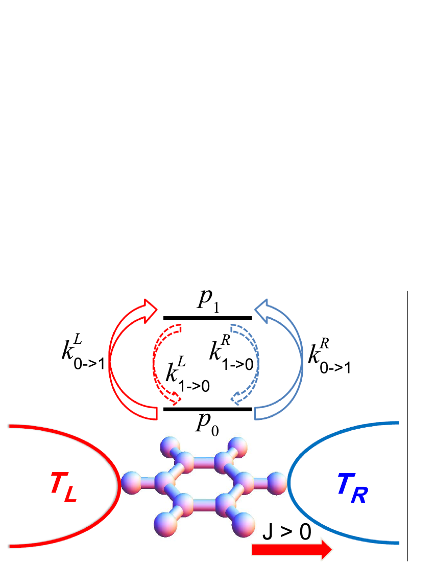
Figure 1: (Color online) A schematic representation of the anharmonic molecular junction. Quantum heat transfer is generated via a dynamics of excitation and relaxation of the local single mode. The heat flux $J$ from the center to the right bath is defined as positive.

In the context of time-dependent manipulations various molecular heat pumps have been proposed to efficiently control heat flux against thermal gradients at the nanoscale. In all those cases the system is driven far away from equilibrium by use of an external modulation imposed on system parameters. For example, a molecular model with modulated energy levels, has been found to operate as a heat pump Segal0608 . Likewise, a spin system leading to the heat pumping has been studied with Ref. Dhar07 . Other schemes investigated pumping of heat in electronic nanoscale devices by applying time-periodic laser fields REY07 . Moreover, Brownian heat motors fueled by oscillating temperatures have recently been devised as well Li0809 ; Ren09 . Given such time-dependent manipulations one may therefore scrutinize whether the physics of a non-vanishing geometric phase does impact the transfer of heat under external modulations. If so, what is its impact on the existence of a heat-flux FT?

In this Letter, we shall answer these above mentioned objectives by studying quantum heat transport across an anharmonic molecular junction model. We start with a system consisting of a molecular junction coupled to two thermal baths Segal0608 , as illustrated in Fig. 1. The total Hamiltonian $H_{tot}$ is composed of the following contributions: $H_{tot}=H_{S}+H^{L}_{B}+H^{R}_{B}+V^{L}_{SB}+V^{R}_{SB}$: system Hamiltonian $H_{S}=\sum_{n=0}^{N-1}E_{n}|n\rangle\langle n|$, with $E_{n}=n\hbar\omega_{0},$ where we assume that heat transport is dominated by a single mode and thus consider a two-level system ($N=2$) to simulate the strong nonlinearity mastereq . If $N\rightarrow\infty$, the system reduces to the quantum harmonic case. The two thermal baths are represented by sets of independent harmonic modes, i.e., $H^{\nu}_{B}=\sum_{k}\hbar\omega_{k}b_{k,\nu}^{\dagger}b_{k,\nu}$, with $\nu=L,R$, where $b_{k,\nu}^{\dagger},b_{k,\nu}$ are the bosonic creation and annihilation operators associated with the phonon mode $k$ of bath $\nu$. The system-bath interactions is taken to be bilinear, i.e., $V^{\nu}_{SB}=B_{\nu}\sum_{n=1}^{N-1}\sqrt{n}|n\rangle\langle n-1|+\mathrm{c.c.}$, $B_{\nu}=\sum_{k}\gamma_{k,\nu}(b^{\dagger}_{k,\nu}+b_{k,\nu})$, where the system-bath interaction is characterized by the phonon spectral function $\Gamma_{\nu}(\omega)=2\pi\sum_{k}\gamma_{k,\nu}^{2}\delta(\omega-\omega_{k})$. In the following, we use wide-band limit $\Gamma_{\nu}(\omega)=\Gamma_{\nu}$. As shown with Ref. mastereq , in the limit of fast dephasing and using the Redfield approximation for weak system-bath coupling, the underlying dynamics can be modeled as follows:

$$\dot{p}_{1}(t)=-p_{1}(t)(k^{L}_{1\rightarrow 0}+k^{R}_{1\rightarrow 0})+p_{0}(t)(k^{L}_{0\rightarrow 1}+k^{R}_{0\rightarrow 1}).$$ (1)

Here, $p_{n}(n=0,1)$ denotes the probability of the molecule to occupy the state $|n\rangle$, satisfying $p_{0}(t)+p_{1}(t)=1$. The activation and relaxation rates read:

$$k^{\nu}_{0\rightarrow 1}=\Gamma_{\nu}N_{\nu}(\omega_{0}),\quad k^{\nu}_{1\rightarrow 0}=\Gamma_{\nu}[N_{\nu}(\omega_{0})+1],$$ (2)

where $N_{\nu}(\omega_{0})=[e^{\beta_{\nu}\hbar\omega_{0}}-1]^{-1}$ is the Bose-Einstein occupation probability. Finally, the steady-state heat flux at the right contact (being equal to the heat flux at the left contact) is expressed as

$$J=\hbar\omega_{0}[p_{1}^{s}k^{R}_{1\rightarrow 0}-p_{0}^{s}k^{R}_{0\rightarrow 1}],$$ (3)

where the superscript $s$ means the steady state. The first term denotes the energy flux going from the molecule into the bath $R$ while the second term provides the opposite heat flux from the bath $R$ back into the system.

Geometric Berry Phase induced Heat Pumping. For heat pump operation, the molecular junction connected to the two reservoirs is subjected to cyclic parameter modulations. This could be realized by imposing a modulation on either of the following parameters: $\omega_{0}(t)$, $\Gamma_{L}(t)$, $\Gamma_{R}(t)$, $T_{L}(t)$, $T_{R}(t)$. Throughout the following, the modulations acting on such system parameters are assumed to be slow, i.e., we employ adiabatic modulations. Let the period of modulation be $\mathcal{T}_{p}=2\pi/\Omega$. The typical frequency for a carbon-carbon bond is $1.4\times 10^{14}s^{-1}$ carbon . $\Gamma_{\nu}$ is around $10^{15}s^{-1}$, according to the measurement with alkane molecular junction Alkane . The relaxation time for fast thermalization usually is on the order of a few fs or ps. Thus, the modulation time scale must obey $2\pi/\Omega\gg 1$ ps. In this way, the assumption of adiabatic modulation is valid whenever the driving frequency $\Omega\ll 1$ THz.

Of prime interest is the heat flux from the molecule into the bath $R$ during the long time span $\tau$. This is achieved upon introducing the characteristic function for the phonon counting field $\chi$, i.e., Gopich06 ; Sinitsyn07a

$$\mathcal{Z}_{\tau}(\chi)=\sum_{q=-\infty}^{\infty}P_{\tau}(q)e^{iq\chi}=\mathbf{1}^{{\dagger}}\hat{T}\left[e^{-\int^{\tau}_{0}\mathcal{H}(\chi,t)dt}\right]\mathbf{p}(0),$$ (4)

$$\mathcal{H}(\chi,t)\doteq\left[\begin{array}[]{cc}k^{L}_{0\rightarrow 1}+k^{R}_{0\rightarrow 1}&-k^{L}_{1\rightarrow 0}-k^{R}_{1\rightarrow 0}e^{i\chi}\\ -k^{L}_{0\rightarrow 1}-k^{R}_{0\rightarrow 1}e^{-i\chi}&k^{L}_{1\rightarrow 0}+k^{R}_{1\rightarrow 0}\\ \end{array}\right],$$ (7)

where $P_{\tau}(q)$ is the probability distribution of having heat $Q=q\hbar\omega_{0}$ transferred from the molecule into the bath $R$ during time $\tau\rightarrow\infty$. Here, $1^{{\dagger}}=[1,1]$, $\hat{T}$ denotes the time-ordering operator, and $\mathbf{p}(0)=[p_{0}(0),p_{1}(0)]^{T}$ are the intial occupation probabilities. Then, the cumulant generating function is obtained as: $\mathcal{G}(\chi)\equiv\lim\limits_{\tau\rightarrow\infty}\tau^{-1}\ln\mathcal{Z}_{\tau}(\chi),$ which generates the heat current via the relation: $J=\hbar\omega_{0}\left.{\partial\mathcal{G}(\chi)}/{\partial(i\chi)}\right|_{\chi=0}$. Denote by $\lambda_{0}(\chi,t)$ the instantaneous eigenvalue of $\mathcal{H}(\chi,t)$ with the smallest real part and $|\psi_{0}(\chi,t)\rangle$ ($\langle\varphi_{0}(\chi,t)|$) the corresponding normalized right (left) eigenvector. The cumulant generating function takes on the following form, being composed of two parts Sinitsyn07a ; supply , namely:

$$\mathcal{Z}_{\tau}(\chi) = e^{\tau\mathcal{G}}=e^{\tau(\mathcal{G}_{\mathrm{dyn}}+\mathcal{G}_{\mathrm{geom}})},$$ (8)

$$\mathcal{G}_{\mathrm{dyn}} = -\mathcal{T}_{p}^{-1}\int^{\mathcal{T}_{p}}_{0}dt\lambda_{0}(\chi,t),$$ (9)

$$\mathcal{G}_{\mathrm{geom}} = -\mathcal{T}_{p}^{-1}\int^{\mathcal{T}_{p}}_{0}dt\langle\varphi_{0}|\partial_{t}|\psi_{0}\rangle,$$ (10)

The fist contribution $\mathcal{G}_{\mathrm{dyn}}$ presents the temporal average and defines the dynamic heat transfer. This is the only term which survives in the static limit. The second, geometric part $\mathcal{G}_{\mathrm{geom}}$ presents an additional contribution caused by the adiabatic cyclic evolution. As we shall see it is this part which possesses a nontrivial geometric interpretation. Let us rewrite $\mathcal{G}_{\mathrm{geom}}$ as a line integral over the closed contour $\mathcal{R}$ in the parameter space $\mathbf{u}$:

$$\mathcal{G}_{\mathrm{geom}}=-\mathcal{T}_{p}^{-1}\oint_{\mathcal{R}}d\mathbf{u}\cdot\mathcal{A}_{\mathbf{u}},\;\>\>\mathcal{A}_{\mathbf{u}}=\langle\varphi_{0}(\mathbf{u})|\frac{\partial}{\partial_{\mathbf{u}}}|\psi_{0}(\mathbf{u})\rangle.$$ (11)

Thus, this is an analog of a Berry phase Berryphase , which does not contain time $t$ explicitly and only depends on the geometry of the modulation contour in the parameter space $\mathbf{u}$. In the case of two parameters being modulated, say $u_{1},u_{2}$, using Stokes theorem, we find

$$\mathcal{G}_{\mathrm{geom}}=-\mathcal{T}_{p}^{-1}\iint_{\mathcal{S_{R}}}du_{1}du_{2}\mathcal{F}_{u_{1}u_{2}},$$ (12)

where $\mathcal{S_{R}}$ is the integral area enclosed by the contour $\mathcal{R}$.

$$\mathcal{F}_{u_{1}u_{2}}=\langle\partial_{u_{1}}\varphi_{0}|\partial_{u_{2}}\psi_{0}\rangle-\langle\partial_{u_{2}}\varphi_{0}|\partial_{u_{1}}\psi_{0}\rangle$$ (13)

is an analog of the gauge invariant Berry curvature Berryphase .

Figure 2: (Color online) (a) The contour map of $-\partial\mathcal{F}_{T_{L}T_{R}}(\chi)/\partial(i\chi)|_{\chi=0}$, for $\Gamma_{L}=\Gamma_{R}$ and $\hbar\omega_{0}=25$ meV. The (blue) circle with an arrow denotes the path of two-parameter temperature modulations: $T_{L}(t)=200+100\cos(\Omega t+\pi/4)$, $T_{R}(t)=200+100\sin(\Omega t+\pi/4)$. The integral area $\mathcal{S_{R}}$ is within the circle. (b) Pure Berry-phase induced heat current: $J_{\mathrm{tot}}=J_{\mathrm{geom}}$ ($J_{\mathrm{dyn}}=0$). The straight line is the analytical result from Eq. (16), while the open circles give the simulation results by integrating Eq. (1).

Let us next specify the case that the bath temperatures $T_{L}(t),T_{R}(t)$ are subjected to adiabatic modulations. Then Eq. (13) yields the Berry curvature in temperature space, reading:

$$\mathcal{F}_{T_{L}T_{R}}(\chi)=-C_{L}C_{R}\frac{2i\sin(\chi)\Gamma_{L}\Gamma_{R}(\Gamma_{L}+\Gamma_{R})}{(\sqrt{K^{2}+4D})^{3}},$$ (14)

where $C_{\nu}=k_{B}\beta^{2}_{\nu}\hbar\omega_{0}e^{\beta_{\nu}\hbar\omega_{0}}N^{2}_{\nu}$, $K=\Gamma_{L}(1+2N_{L})+\Gamma_{R}(1+2N_{R})$, $D=\Gamma_{L}\Gamma_{R}N_{L}N_{R}(e^{\beta_{R}\hbar\omega_{0}}e_{+\chi}+e^{\beta_{L}\hbar\omega_{0}}e_{-\chi})$ with $e_{\pm\chi}\equiv e^{\pm i\chi}-1$. Upon substituting this Berry curvature into Eq. (12), the total heat flux emerges as:

$$J_{\mathrm{tot}}=\hbar\omega_{0}\left.\frac{\partial[\mathcal{G}_{\mathrm{dyn}}(\chi)+\mathcal{G}_{\mathrm{geom}}(\chi)]}{\partial(i\chi)}\right|_{\chi=0}=J_{\mathrm{dyn}}+J_{\mathrm{geom}},$$

$$J_{\mathrm{dyn}}=\frac{\hbar\omega_{0}}{\mathcal{T}_{p}}\int^{\mathcal{T}_{p}}_{0}dt\frac{\Gamma_{L}\Gamma_{R}(N_{L}-N_{R})}{K},$$ (15)

$$J_{\mathrm{geom}}=\frac{\hbar\omega_{0}}{\mathcal{T}_{p}}\iint_{\mathcal{S_{R}}}dT_{L}dT_{R}\left.\frac{-\partial\mathcal{F}_{T_{L}T_{R}}(\chi)}{\partial(i\chi)}\right|_{\chi=0},$$ (16)

where

$$\left.-\frac{\partial\mathcal{F}_{T_{L}T_{R}}(\chi)}{\partial(i\chi)}\right|_{\chi=0}=\frac{2C_{L}C_{R}\Gamma_{L}\Gamma_{R}(\Gamma_{L}+\Gamma_{R})}{K^{3}}.$$ (17)

The dynamic part $J_{\mathrm{dyn}}$ just coincides with the temporal average of the heat flux obtained from $J\equiv J(t)$ in Eq. (3). The geometric part $J_{\mathrm{geom}}$ is the additional heat flux that results from the nontrivial Berry phase effect. The ratio of this geometric heat flux and the dynamic one is typically about $\Omega/\Gamma_{\nu}$. To avoid that $J_{\mathrm{geom}}$ is masked by $J_{\mathrm{dyn}}$, we choose a symmetric molecular junction with $\Gamma_{L}=\Gamma_{R}$, and modulate $T_{L}(t),T_{R}(t)$ as indicated by the circle contour in Fig. 2a. Then one finds that $J_{\mathrm{dyn}}\equiv 0$ and $J_{\mathrm{geom}}\neq 0$, see Fig. 2b, so that the Berry phase induced $J_{\mathrm{geom}}$ dominates the heat transport. This is the case for which the geometric phase effect on heat transport is distinctly experimentally detectable. As a main finding we have that the Berry phase effect acts as a heat pump, providing an additional heat flux across the molecular junction even though on average no thermal bias acts and the system is symmetric. Note also, distinct from the irreversible heat flux $J_{\mathrm{dyn}}$, $J_{\mathrm{geom}}$ is time-reversible, i.e., under the time-reversed modulation ($t\rightarrow-t$) the Berry-phase induced heat flux just reverses sign.

Fractional Quantization of Phonon Response. Remarkably, we find a fractional quantized phonon response for large temperature driving: the integral in Eq. (16) can be rewritten as $\int^{\infty}_{0}\int^{\infty}_{0}dN_{L}dN_{R}2\Gamma_{L}\Gamma_{R}(\Gamma_{L}+\Gamma_{R})/K^{3}=1/4$, yielding supply :

$$J_{\mathrm{geom}}=\frac{1}{4}\hbar\omega_{0}/\mathcal{T}_{p}.$$ (18)

This $1/4$ fractional quantized geometric phonon response is robust since it does not depend on the specific values of $\hbar\omega_{0},\Gamma_{L},\Gamma_{R}$. It means that the geometric phase effect caused by two bath temperature modulations is able to pump maximally on average one phonon $\hbar\omega_{0}$ per four cycles.

Impact on Heat-Flux Fluctuation Theorem. Besides the dynamic $\mathcal{G}_{\mathrm{dyn}}$, $\mathcal{G}_{\mathrm{geom}}$ will generally not only contribute additionally to the average heat transfer but also impact the higher moments of the heat current (such as the phonon counting statistics) and other heat transport characteristics as well. In the following, we study its impact on the heat-flux fluctuation theorem. Before doing so, let us address first the static situation with $\mathcal{G}_{\mathrm{geom}}(\chi)\equiv 0$, yielding

$$\mathcal{G}(\chi)=\mathcal{G}_{\mathrm{dyn}}(\chi)=-\lambda_{0}(\chi)=\frac{-K+\sqrt{K^{2}+4D}}{2}.$$ (19)

Then, $\lambda_{0}$ obeys the Gallavotti-Cohen (GC) symmetry Lebowitz99 (and alike for $\mathcal{G}_{\mathrm{dyn}}(\chi)$, $\mathcal{G}(\chi)$ and $\mathcal{Z}_{\tau}(\chi)$), reading

$$\mathcal{\lambda}_{0}(\chi)=\mathcal{\lambda}_{0}(-\chi+i\beta^{*}),$$ (20)

where $\beta^{*}=\ln[(k^{L}_{0\rightarrow 1}k^{R}_{1\rightarrow 0})/(k^{R}_{0\rightarrow 1}k^{L}_{1\rightarrow 0})]$. In virtue of Eq. (2), yielding the detailed balance relation $k^{\nu}_{0\rightarrow 1}=k^{\nu}_{1\rightarrow 0}e^{-\beta_{\nu}\hbar\omega_{0}},$ we find that $\beta^{*}=\hbar\omega_{0}(\beta_{R}-\beta_{L})$. Via an inverse Fourier transform of Eq. (4), this GC symmetry results in the quantum FT of heat transport for an anharmonic molecular junctions, reading with $Q=q\hbar\omega_{0}$:

$$\lim\limits_{\tau\rightarrow\infty}\frac{1}{\tau}\ln[\frac{P_{\tau}(Q)}{P_{\tau}(-Q)}]=Q(\beta_{R}-\beta_{L})/\tau,$$ (21)

which precisely coincides (without any correction) with the result for the quantum harmonic chain Saito07 . This FT gives the probability of observing spontaneous “second law violation”: Assume $T_{L}<T_{R}$, i.e. $\beta^{*}<0$; the upper bound to observe the “violation” for spontaneous heat transfer from (left) cool to (right) hot is estimated as: $\int^{\infty}_{c}dqP_{\tau}(q)=\int^{\infty}_{c}dqP_{\tau}(-q)e^{q\beta^{*}}\leq e^{c\beta^{*}}.$ It indicates that in absence of external modulations, the probability of at least $c$ phonons (or net energy $c\hbar\omega_{0}$) transporting against the thermal bias is nonvanishing detectable, although decaying exponentially.

For the time-modulated system the GC symmetry ceases to hold when $\mathcal{G}_{\mathrm{geom}}(\chi)\neq 0$. For example, in the case of cyclic temperature modulations $T_{L}(t)$ and $T_{R}(t)$, the Berry curvature $\mathcal{F}_{T_{L}T_{R}}(\chi)$ contains the factor $\sin(\chi)$, which explicitly breaks the GC symmetry of $\mathcal{G}_{\mathrm{geom}}(\chi)$, and alike for $\mathcal{G}(\chi)$ and $\mathcal{Z}_{\tau}(\chi)$. Thus, the FT Eq. (21) becomes violated as a consequence of a geometric phase induced breakdown of GC symmetry. Moreover, even for parameter modulations yielding $\mathcal{G}_{\mathrm{geom}}(\chi)=0$, and with time-dependent $\beta^{*}\rightarrow\beta^{*}(t)$, the GC symmetry for $\mathcal{G}_{\mathrm{dyn}}(\chi)=-\mathcal{T}^{-1}_{p}\int^{\mathcal{T}_{p}}_{0}dt\lambda_{0}(\chi,t)$ generally cannot be recovered, despite $\lambda_{0}(\chi,t)=\lambda_{0}(-\chi+i\beta^{*}(t),t)$.

Interestingly, we find that for time modulations of the system-bath couplings $\Gamma_{L}(t),\Gamma_{R}(t)$, the detailed balance relation $k^{\nu}_{0\rightarrow 1}/k^{\nu}_{1\rightarrow 0}=e^{-\beta_{\nu}\hbar\omega_{0}}$ remains intact, thus providing a vanishing Berry curvature $\mathcal{F}_{\Gamma_{L}\Gamma_{R}}(\chi)\equiv 0$. Meanwhile, with the resulting time-independent $\beta^{*}(t)=\beta^{*}$, one finds that the GC symmetry of $\mathcal{G}_{\mathrm{dyn}}(\chi)=-\mathcal{T}_{p}^{-1}\int^{\mathcal{T}_{p}}_{0}dt\lambda_{0}(\chi,t)$ still holds. Consequently, we obtain a vanishing Berry-phase induced heat pumping and, surprisingly as well, also no violation of the FT, no matter how $\Gamma_{L}(t)$ and $\Gamma_{R}(t)$ are modulated.

In summary, through investigating heat transport across an anharmonic molecular junction by applying cyclic two-parameter modulations, we find that the system generally undergoes, apart from dynamic pumping, also a Berry phase induced heat pumping. This geometric contribution exhibits a robust fractional quantized phonon response. Furthermore, the quantum FT for heat transport in presence of a static temperature bias holds true in the anharmonic case as well. The presence of the geometric phase, however, violates the heat-flux FT. Only in situations of vanishing Berry curvature and restoration of detailed balance symmetry can the validity of the FT be recovered.

Although our present work did focus on the adiabatic regime, it likely can be extended to the case of a non-adiabatic geometric phase Ohkubo , and maybe also for non-cyclic modulation schemes in the spirit of Sinitsyn07b . Because the geometric phase has profound effects on material properties Berryphase we hope that our present findings do invigorate others to undertake related studies aimed at uncovering intriguing novel geometric phase induced thermal effects (such as thermoelectricity) which will enrich further the discipline of phononics.

The work is supported by the grant R-144-000-222-646 from National University of Singapore (NUS) (J.R. and B.L.) and by the German Excellence Initiative via the Nanosystems Initiative Munich (NIM) and DFG priority program SPP 1243 (P.H.).

I Supplementary Information of “Berry-Phase induced Heat Pumping and its Impact on the Fluctuation Theorem”

I.1 The Generating Function with the Phonon Counting Field and associated Geometric Phase

In this section, we derive the geometric phase effect from time evolution of the generating function with phonon counting fields in more detailed form. For our system, $P_{t}(q)$ denotes the probability that within time $t$ the net number of phonons transferred from the molecule into the bath $R$ is $q$. We then split this probability into two parts, namely, $P_{t}(q)\doteq P_{t}(0,q)+P_{t}(1,q)$, where $P_{t}(0,q)$ $(P_{t}(1,q))$ denotes the probability that having $q$ net phonons transferred from the molecule into the bath $R$, within time $t$, while the molecule is dwelling on the low “0” (high “1”) energy level at time $t$. The time evolution of our system can be described as:

$$\frac{d}{dt}P_{t}(0,q) = -(k^{L}_{0\rightarrow 1}+k^{R}_{0\rightarrow 1})P_{t}(0,q)+k^{L}_{1\rightarrow 0}P_{t}(1,q)+k^{R}_{1\rightarrow 0}P_{t}(1,q-1),$$

$$\frac{d}{dt}P_{t}(1,q) = k^{L}_{0\rightarrow 1}P_{t}(0,q)+k^{R}_{0\rightarrow 1}P_{t}(0,q+1)-(k^{L}_{1\rightarrow 0}+k^{R}_{1\rightarrow 0})P_{t}(1,q).$$

By multiplying the factor $e^{iq\chi}$ on both sides of the equations and summing over $q$, we obtain the time evolution equation of these individual generating functions:

$$\frac{d}{dt}|\Psi(\chi,t)\rangle=-\mathcal{H}(\chi,t)|\Psi(\chi,t)\rangle,$$

where

$$\mathcal{H}(\chi,t)=\left[\begin{array}[]{cc}k^{L}_{0\rightarrow 1}+k^{R}_{0\rightarrow 1}&-k^{L}_{1\rightarrow 0}-k^{R}_{1\rightarrow 0}e^{i\chi}\\ -k^{L}_{0\rightarrow 1}-k^{R}_{0\rightarrow 1}e^{-i\chi}&k^{L}_{1\rightarrow 0}+k^{R}_{1\rightarrow 0}\\ \end{array}\right],\;\;\;\;\;\;|\Psi(\chi,t)\rangle=\left(\begin{array}[]{c}\sum^{\infty}_{q=-\infty}P_{t}(0,q)e^{iq\chi}\\ \sum^{\infty}_{q=-\infty}P_{t}(1,q)e^{iq\chi}\\ \end{array}\right).$$

Therefore, the characteristic function $\mathcal{Z}_{\tau}(\chi)$ emerges as:

$$\mathcal{Z}_{\tau}(\chi)\equiv\sum^{\infty}_{q=-\infty}P_{\tau}(q)e^{iq\chi}=\mathbf{1}^{{\dagger}}|\Psi(\chi,\tau)\rangle=\mathbf{1}^{{\dagger}}\hat{T}\left[e^{-\int^{\tau}_{0}\mathcal{H}(\chi,t)dt}\right]|\Psi(\chi,0)\rangle.$$

At initial $t=0$, the net number of transferred phonons is $0$, thus $|\Psi(\chi,0)\rangle=[p_{0}(t=0),p_{1}(t=0)]^{T}$. Note that the time evolution equation Eq. (S1) for generating functions including the counting field exists for systems described by such master equations generallyGopich2006 .

In the following, we are going to derive the geometric phase from the time evolution of the generating function (we omit the counting field variable $\chi$ for the sake of better readability). We stress that the time-dependent operator $\mathcal{H}(t)$ is not a genuine, hermitian Hamilton operator. However, we still can decompose it as

$$\mathcal{H}(t)|\psi_{n}(t)\rangle=\lambda_{n}(t)|\psi_{n}(t)\rangle,\;\;\;\;\;\;\langle\varphi_{n}(t)|\mathcal{H}(t)=\langle\varphi_{n}(t)|\lambda_{n}(t),$$

where $\lambda_{n}(t)$ denotes the instantaneous eigenvalue of $\mathcal{H}(t)$ and $|\psi_{n}(t)\rangle$ $(\langle\varphi_{n}(t)|)$ the corresponding normalized right (left) eigenvector, satisfying $\langle\varphi_{m}(t)|\psi_{n}(t)\rangle=\delta_{mn}$. Similar to Berry’s reasoning Berry1984 , we expand $|\Psi(t)\rangle$ as

$$|\Psi(t)\rangle=\sum_{n}a_{n}(t)\exp\left(-\int^{t}_{0}\lambda_{n}(t^{\prime})dt^{\prime}\right)|\psi_{n}(t)\rangle.$$

By substituting Eq. (S3) into the time evolution equation Eq. (S1), we find

$$\sum_{n}\dot{a}_{n}(t)\exp\left(-\int^{t}_{0}\lambda_{n}(t^{\prime})dt^{\prime}\right)|\psi_{n}(t)\rangle=\sum_{n}a_{n}(t)\exp\left(-\int^{t}_{0}\lambda_{n}(t^{\prime})dt^{\prime}\right)|\dot{\psi}_{n}(t)\rangle.$$

Upon the multiplication of the left eigenvector $\langle\varphi_{m}(t)|$ and observing that $\langle\varphi_{m}(t)|\psi_{n}(t)\rangle=\delta_{mn}$, we obtain

$$\dot{a}_{m}(t)=-a_{m}(t)\langle\varphi_{m}(t)|\dot{\psi}_{m}(t)\rangle-\sum_{n\neq m}a_{n}(t)\exp\left(-\int^{t}_{0}[\lambda_{n}(t^{\prime})-\lambda_{m}(t^{\prime})]dt^{\prime}\right)\langle\varphi_{m}(t)|\dot{\psi}_{n}(t)\rangle.$$

Note $\lambda_{n}$ are complex-valued eigenvalues. The long time behavior of the system is governed by the eigenmode $m=0$, whose eigenvalue $\lambda_{0}$ possesses the smallest real part. Consequently, by neglecting the last term within our adiabatic approximation, one obtains:

$$a_{0}(\tau)=\exp\left(-\int^{\tau}_{0}\langle\varphi_{0}|\dot{\psi}_{0}\rangle dt\right)a_{0}(0),\;\>\>\tau\rightarrow\infty.$$

Taking into account the adiabatic cyclic evolution over a long-time period $\mathcal{T}_{p}$, we end up with

$$\mathcal{Z}_{\tau}=\mathbf{1}^{{\dagger}}|\Psi(\tau)\rangle\approx\exp\left(-\frac{\tau}{\mathcal{T}_{p}}\int^{\mathcal{T}_{p}}_{0}dt\left[\lambda_{0}(t)+\langle\varphi_{0}|\dot{\psi}_{0}\rangle\right]\right)a_{0}(0)\mathbf{1}^{{\dagger}}|\psi_{0}(\tau)\rangle,$$

which tells us that the cumulant generating function $\mathcal{G}(\chi)\equiv\lim\limits_{\tau\rightarrow\infty}\tau^{-1}\ln\mathcal{Z}_{\tau}(\chi)=\mathcal{G}_{\mathrm{dyn}}+\mathcal{G}_{\mathrm{geom}}$ contains two contributions, one originating from the dynamic phase factor and the other from the geometric phase factor (the boundary value contribution: $\tau^{-1}\ln\left[a_{0}(0)\mathbf{1}^{{\dagger}}|\psi_{0}(\tau)\rangle\right]$ becomes negligible in the long time limit):

$$\mathcal{G}_{\mathrm{dyn}}=-\mathcal{T}_{p}^{-1}\int^{\mathcal{T}_{p}}_{0}dt\lambda_{0}(\chi,t),$$

$$\mathcal{G}_{\mathrm{geom}}=-\mathcal{T}_{p}^{-1}\int^{\mathcal{T}_{p}}_{0}dt\langle\varphi_{0}|\partial_{t}|\psi_{0}\rangle.$$

These two expressions of $\mathcal{G}_{\mathrm{dyn}}$ and $\mathcal{G}_{\mathrm{geom}}$ coincide precisely with those obtained in Ref. Sinitsyn2007a , although derived therein using a different approach.

I.2 Fractional Quantized Phonon Response

Now, we give a detailed explanation of the physical picture of the observed $1/4$ fractional quantized phonon response, in particular, the cause of the Berry phase effect induced by temperature modulations of the two heat baths to transfer on average $1/4$ phonon $\hbar\omega_{0}$ per one modulation cycle.

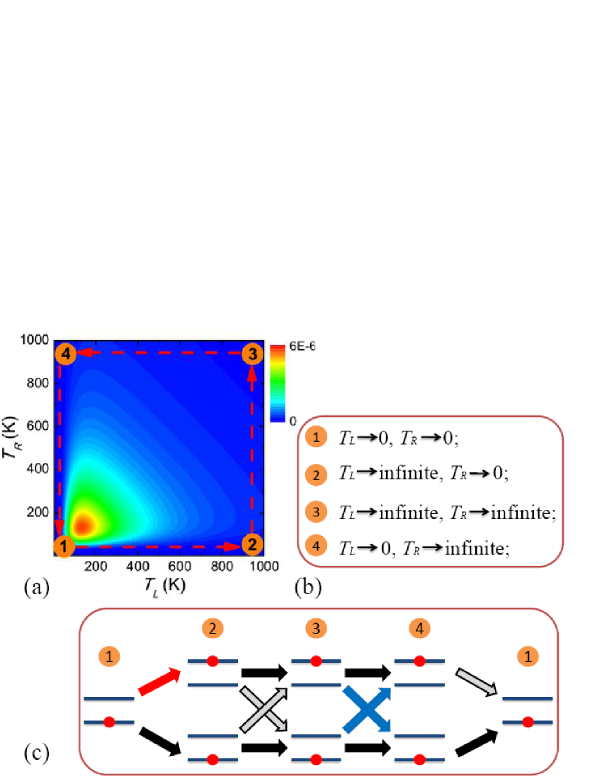
Figure 3: (Color online) A schematic representation of the temperature modulation cycle and corresponding level transitions. (a)The contour map of $-\partial\mathcal{F}_{T_{L}T_{R}}(\chi)/\partial(i\chi)|_{\chi=0}$, for $\Gamma_{L}=\Gamma_{R}$ and $\hbar\omega_{0}=25$ meV. The (red) dash line with an arrow denotes the trajectory of temperature modulations. (b)The temperature list of state (1)(2)(3)(4). (c) The corresponding transitions during cycle $(1)\rightarrow(2)\rightarrow(3)\rightarrow(4)\rightarrow(1)$. The red arrow denotes only the up transition from bath $L$ is excited; while the transitions only allowed at the $R$ bath are indicated by blue arrows. Besides, black arrows indicate that the system stays intact and gray arrows depict the transitions occurring at both $L$ and $R$ bath with equal probability.

Mathematically, when the integral area $\mathcal{S_{R}}$ due to the two parameter modulation encloses a large part of the area around the maximum of $-\partial\mathcal{F}_{T_{L}T_{R}}(\chi)/\partial(i\chi)|_{\chi=0}$, or, put differently for strong temperature driving temperature comprising near zero temperature up to large values beyond $\hbar\omega_{0}$, as sketched by the dashed path in Fig. 3a, the integral in $J_{\mathrm{geom}}$ can be recast as

$$J_{\mathrm{geom}}=\frac{\hbar\omega_{0}}{\mathcal{T}_{p}}\int^{\infty}_{0}\int^{\infty}_{0}dN_{L}dN_{R}\frac{2\Gamma_{L}\Gamma_{R}(\Gamma_{L}+\Gamma_{R})}{K^{3}}=\frac{1}{4}{\hbar\omega_{0}}/{\mathcal{T}_{p}},$$

The underlying physical mechanism is as the following: As shown in Fig. 3a, the trajectory of this so obtained temperature modulation follows the path: $(1)\rightarrow(2)\rightarrow(3)\rightarrow(4)\rightarrow(1)$, where (1) ($T_{L}=0,T_{R}=0$), (2) ($T_{L}=0,T_{R}\rightarrow\infty$), (3) ($T_{L}\rightarrow\infty,T_{R}\rightarrow\infty$), (4) ($T_{L}\rightarrow\infty,T_{R}=0$) as detailed in Fig. 3b. For the two-level system under consideration, only for the parameter set around (1) does the system fully occupy the lower level; at the other three sets (2), (3), (4), the system occupies the upper level and lower one with equal probability. The level transitions during the course of the temperature modulation are illustrated with Fig. 3c. Usually, the transition from the lower (upper) level to the upper (lower) contain two parts of contributions: one is from the left bath and the other is from the right bath, respectively (see Fig. 1 in the text). However, for the transition from (1) to (2), the temperature of bath $L$ is increased from $0$ to $\infty$ so that only the up transition from bath $L$ is excited, which is indicated as the red arrow; while for the transition from (3) to (4), $T_{L}$ is modulated near zero and $T_{R}$ keeps extremely high so that only the transitions from the $R$ bath become allowed. Those are indicated as blue arrows (see Fig. 3c). Besides, black arrows indicate that the system stays intact and gray arrows depict the transitions occurring at either $L$ or $R$ bath with equal probability. Note that only the up transition at $L$ followed by one down transition at $R$ counts for the positive energy transport from $L$ to $R$.

The transitions during temperature modulations can be further decomposed into eight individual paths, as illustrated in Fig. 4. Therefore, we can count the amount of energy transport for each path individually. For example, in path (a), the up transition is excited at $L$ during $(1)\rightarrow(2)$, and then the system keeps in the upper level until the down transition happens during $(4)\rightarrow(1)$. Since the down transition exhibit a splitting, occurring at $L$ or $R$, this path contributes $1/2$ phonon for the energy transport. In path (b), the up transition at $L$ is first excited and then during $(3)\rightarrow(4)$ the down transition occurs at $R$, so that one phonon is transported during the whole modulation cycle. The amount of energy transport in other paths can be accounted likewise.

Finally, the total amount of phonon transport during one temperature modulation cycle is expressed as the average of contributions from these eight routes:

$$\frac{1/2+1+0+1/2+0+(-1/2)+0+1/2}{8}=\frac{1}{4}.$$

In other words, after one complete modulation cycle, the system returns to its “original” state but with $\hbar\omega_{0}/4$ energy given away. This effect has a geometric interpretation and can be utilized to act as a heat pump.

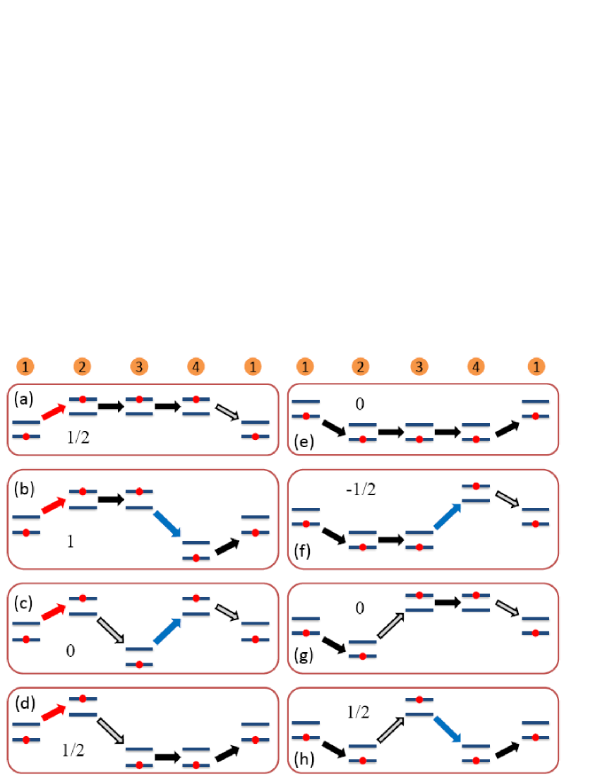
Figure 4: (Color online) Decomposition of the level transitions into eight individual transition paths. The amount of phonon transport contributed by each path is indicated.

In summary, this scenario makes it plausible that the Berry phase effect caused by two-parameter temperature modulations is able to induce on average a heat transfer across the molecular junction in the amount of $1/4$ phonon $\hbar\omega_{0}$ per modulation cycle. This $1/4$ fractional quantized phonon response is robust in the sense that it does not depend on the specific values of $\hbar\omega_{0},\Gamma_{L},\Gamma_{R}$.

References

(1) L. Wang and B. Li, Physics World 21, 27 (2008).
(2) C. W. Chang, D. Okawa, A. Majumdar, and A. Zettl, Science 314, 1121 (2006).
(3) C. W. Chang, D. Okawa, H. Garcia, A. Majumdar, and A. Zettl, Phys. Rev. Lett. 99, 045901 (2007).
(4) B. Li, L. Wang and G. Casati, Appl. Phys. Lett. 88, 143501 (2006).
(5) L.-A. Wu and D. Segal, Phys. Rev. Lett. 102, 095503 (2009).
(6) For comprehensive review see: M. Esposito, U. Harbola, and S. Mukamel, Rev. Mod.
Phys. 81, 1665 (2009).
(7) C. Jarzynski and D. K. Wójcik, Phys. Rev. Lett. 92, 230602
(2004); Y. Sughiyama and S. Abe, J. Stat. Mech.: Theory Exp. P05008, (2008).
(8) K. Saito and A. Dhar, Phys. Rev. Lett. 99, 180601 (2007).
(9)P. Talkner, M. Campisi, and P. Hänggi, J. Stat. Mech.: Theory Exp. P02025, (2009)
(10) D. J. Evans, E. G. D. Cohen, and G. P. Morriss,
Phys. Rev. Lett. 71, 2401 (1993).
(11)G. Gallavotti and E. G. D. Cohen, Phys. Rev. Lett.
74, 2694 (1995).
(12)D. Segal and A. Nitzan, Phys. Rev. E 73, 026109
(2006); D. Segal, Phys. Rev. Lett. 101, 260601 (2008).
(13) R. Marathe, A. M. Jayannavar, and A. Dhar, Phys. Rev. E 75, 030103(R) (2007).
(14) M. Rey, M. Strass, S. Kohler, P. Hänggi, and F. Sols, Phys. Rev. B
76, 085337 (2007); L. Arrachea, M. Moskalets, and L.
Martin-Moreno, Phys. Rev. B 75, 245420, (2007).
(15) N. Li, P. Hänggi, and B. Li, Europhys. Lett. 84, 40009
(2008); N. Li, F. Zhan, P. Hänggi, and B. Li, Phys. Rev. E 80, 011125 (2009); F. Zhan, N. Li, S. Kohler, and P. Hänggi,
Phys. Rev. E 80, 061115 (2009).
(16) J. Ren and B. Li, Phys. Rev. E 81, 021111
(2010).
(17) D. Segal, Phys. Rev. B, 73 205415 (2006).
(18) J. Grunenberg, Angew. Chem. Int. Ed. 40,
4027 (2001).
(19) Z. Wang, J. A. Carter, A. Lagutchev, Y. K. Koh,
N. Seong, D. G. Cahill, and D. D. Dlott, Science 317, 787
(2007).
(20) I. V. Gopich and A. Szabo, J. Chem. Phys.
124, 154712 (2006).
(21) N. A. Sinitsyn and I. Nemenman,
Europhys. Lett. 77, 58001 (2007).
(22) For the detailed derivation of the geometric phase contribution in
generating functions and detailed explanations of the physical
picture of the fractional quantized phonon response, please
see EPAPS Document.
(23) A. Bohm, A. Mostafazadeh, H. Koizumi, Q. Niu, and
J. Zwanziger, The Geometric Phase in Quantum Systems,
(Springer-Verlag, New York, 2003).
(24) J. L. Lebowitz and H. Spohn, J. Stat. Phys. 95 333 (1999).
(25) J. Ohkubo, J. Stat. Mech.: Theory Exp. P02011, (2008).
(26) N. A. Sinitsyn, J. Phys. A: Math. Theor. 42, 193001 (2009).

References

(1) I. V. Gopich and A. Szabo, J. Chem. Phys.
124, 154712 (2006).
(2) M. V. Berry, Proc. R. Soc. Lond. A 392, 45
(1984).
(3) N. A. Sinitsyn and I. Nemenman,
Europhys. Lett. 77, 58001 (2007).