Topological effect on spin transport in a magnetic quantum wire: Green’s function approach

Abstract

We explore spin dependent transport through a magnetic quantum wire which is attached to two non-magnetic metallic electrodes. We adopt a simple tight-binding Hamiltonian to describe the model where the quantum wire is attached to two semi-infinite one-dimensional non-magnetic electrodes. Based on single particle Green’s function formalism all the calculations are performed numerically which describe two-terminal conductance and current-voltage characteristics through the wire. Quite interestingly we see that, beyond a critical system size probability of spin flipping enhances significantly that can be used to design a spin flip device. Our numerical study may be helpful in fabricating mesoscopic or nano-scale spin devices.

I Introduction

Over the past two decades spin dependent transport in low-dimensional systems has emerged as one of the most extensively cultivated area in condensed matter physics, due to its potential application in the fields of nanoelectronics and nanotechnology nano1 ; nano2 . Introduced in $1996$, by S. Wolf, the term ‘spintronics’ spintronics1 ; spintronics2 ; spintronics3 refers to a new branch in physics that deals with control and manipulation of electron spin in addition to its charge for storage and transfer of information as in conventional electronics. Idea of possibility to exploit electron spin in transport phenomena was ignited by the discovery of giant magneto-resistance (GMR) effect gmr in Fe/Cr magnetic multi-layers in $1980$’s and it holds future promises of integrating memory and logic into a single device. Since the discovery of GMR based magnetic field sensors, revolutionary development has taken place in magnetic data storage applications, device processing techniques, and quantum computation. ‘Spintronics’ presents a new paradigm in quantum computation with incredible speed up in computational time and much reduced complexity in quantum-computing algorithm, using the idea of quantum coherence and spin entanglement. The key idea of spintronic applications involves three basic steps that are injection of spin through interfaces, transmission of spin through matter, and finally detection of spin. Having considerably larger spin diffusion length molecules and quantum confined nanostructures e.g., quantum dots are ideal candidates to study spin dependent transmission. Therefore, from technological as well as theoretical point of view study of spin transport in mesoscopic regime is of great importance today.

Till date several experimental and theoretical works have been done to investigate spin transport phenomena at nanoscale level. In $2004$ Rohkinson et al. prepared a spin filter rokhinson using GaAs by atomic force microscopy (AFM) with local anodic oxidation and molecular beam epitaxy (MBE) methods. In $2005$, gate field controlled magnetoresistance schonenberger in carbon nanotube with metallic contacts is observed by Schönenberger et al. In $2007$, Tombros et al. studied spin transport in single graphene layer at room temperature tombros . Various other experiments have also been performed in this field. Along with such novel experimental works spin transport in mesoscopic regime has drawn attention from theoretical point of view as well. Present theoretical investigations in this field explores various interesting features e.g., spin dependent conductance modulation condmod , spin filtering filter ; san1 , spin switching switch , spin detecting mechanisms detect , etc. Recently, Shokri et al. have studied spin dependent transmission within the coherent transport regime through magnetic or non-magnetic nanostructures e.g., quantum wire, etc., attached to semi-infinite magnetic or non-magnetic leads using Transfer matrix method and single particle Green’s function formalism shokri1 ; shokri2 ; shokri3 ; shokri4 ; shokri5 . It is observed that the conductance of such mesoscopic systems depends on the spin state of electrons passing through the system and can be controlled by applying external magnetic field shokri6 .

The aim of our present work is to study spin dependent transmission through a magnetic quantum wire. The quantum wire, composed of an array of magnetic atoms, is attached symmetrically to two non-magnetic (NM) semi-infinite one-dimensional ($1$D) metallic electrodes. A simple tight-binding Hamiltonian is used to describe the system where all the calculations are done by using single particle Green’s function formalism san2 ; san3 . With the help of Landauer conductance formula datta1 ; datta2 , spin dependent conductance is obtained, and the current-voltage characteristics are computed from the Landauer-Büttiker formalism land1 ; land2 ; land3 . Here, we explore various features of spin dependent transport using different orientations of local magnetic moments in a magnetic quantum wire. It is interesting to note that, for a specific configuration of local magnetic moments as we will describe latter, spin flip transmission dominates significantly over pure spin transmission after the system size becomes larger than a critical value. This phenomenon can be utilized to desgin a tailor made spin flip device.

The scheme of the paper is as follows. With a brief introduction (Section I), in Section II, we describe the model and theoretical formulation for the calculation. Section III explores the significant results which describe two-terminal conductance and current through the wire and our results clearly depict the spin flipping action depending on the system size. At the end, we conclude our results in Section IV.

II Model and synopsis of the theoretical formulation

We start by describing our model as shown in Fig 1. In this figure we illustrate schematically the $1$D nanostructure through which we are interested to explore several features of spin dependent transport phenomena. In the present work, spin transmission is investigated through

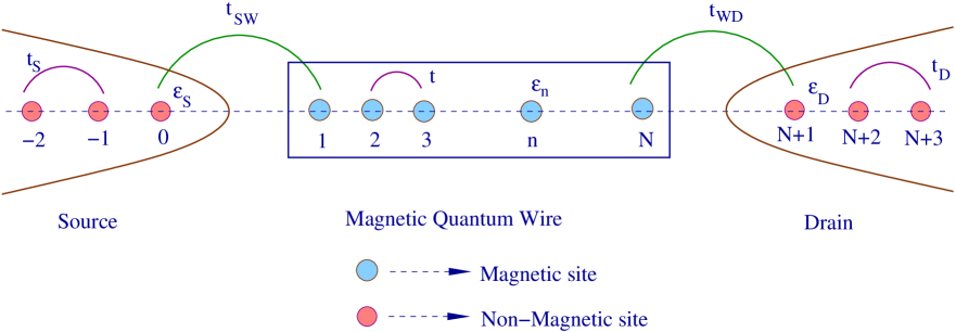
Figure 1: (Color online). A magnetic quantum wire (framed region) of $N$ atomic sites attached to two semi-infinite one-dimensional non-magnetic metallic electrodes, namely, source and drain. The filled sky blue circles correspond to magnetic atomic sites in the quantum wire, while the filled pink circles represent non-magnetic atomic sites comprising the electrodes.

a magnetic quantum wire (MQW) which is basically an array of $N$ number of magnetic atomic sites. Each site has a localized magnetic moment of equal amplitude associated with it. The orientations of the local magnetic moment in a site $n$ (say) are specified by the polar angle $\theta_{n}$ and azimuthal angle $\phi_{n}$ in spherical polar coordinate system and the direction of the moment can be altered by applying an external magnetic field. The QW is attached symmetrically to two $1$D semi-infinite non-magnetic metallic electrodes, commonly termed as source and drain having chemical potentials $\mu_{1}$ and $\mu_{2}$ under the non-equilibrium condition when bias voltage is applied. Described by the discrete lattice model, the electrodes are assumed to be composed of infinite non-magnetic sites labeled as $0$, $-1$, $-2$, $\ldots$, $-\infty$ for the source and $(N+1)$, $(N+2)$, $(N+3)$, $\ldots$, $\infty$ for the drain.

In our present work we consider two different configurations of the MQW depending on the orientation of the localized moments on each site as illustrated in Figs. 2 and 3. In configuration $1$ (see Fig 2), all the magnetic moments are directed along $+Z$ direction and their orientation can be changed in an equal amount by applying an external magnetic field. In configuration $2$ (see Fig 3), the magnetic moments are aligned in a spin wave like pattern with the help of a spatially inhomogeneous external magnetic field.

The Hamiltonian for the whole system can be written as,

$$H=H_{W}+H_{S}+H_{D}+H_{SW}+H_{WD}$$ (1)

where, $H_{W}$ represents the Hamiltonian for the magnetic quantum wire (MQW). $H_{S(D)}$ corresponds to the Hamiltonian for the left (right)

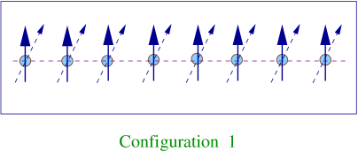
Figure 2: (Color online). Configuration $1$: A magnetic quantum wire with $N$ atomic sites where all magnetic moments are aligned in a particular direction (solid arrows). These moments are rotated equally from their initial directions by applying an external magnetic field (dashed arrows).

electrode, namely, source (drain), and $H_{SW(WD)}$ is the Hamiltonian describing the wire-electrode coupling.

The spin polarized Hamiltonian for the MQW can be written in a single electron picture within the framework of tight-binding formulation in Wannier basis, using nearest-neighbor approximation as,

$$H_{W}=\sum_{n=1}^{N}{\bf c_{n}^{\dagger}\left(\epsilon_{0}-\vec{h_{n}}.\vec{\sigma}\right)c_{n}}+\sum_{i=1}^{N}{\bf\left(c_{i}^{\dagger}tc_{i+1}+h.c.\right)}$$ (2)

where,
${\bf c_{n}^{\dagger}}=\left(\begin{array}[]{cc}c_{n\uparrow}^{\dagger}&c_{n\downarrow}^{\dagger}\end{array}\right);~{}~{}$ ${\bf c_{n}}=\left(\begin{array}[]{c}c_{n\uparrow}\\ c_{n\downarrow}\end{array}\right);~{}~{}$ ${\bf\epsilon_{0}}=\left(\begin{array}[]{cc}\epsilon_{0}&0\\ 0&\epsilon_{0}\end{array}\right)$
${\bf t}=t\left(\begin{array}[]{cc}1&0\\ 0&1\end{array}\right);~{}~{}$ ${\bf\vec{h_{n}}.\vec{\sigma}}=h_{n}\left(\begin{array}[]{cc}\cos\theta_{n}&\sin\theta_{n}e^{-i\phi_{n}}\\ \sin\theta_{n}e^{i\phi_{n}}&-\cos\theta_{n}\end{array}\right)$
 
First term of Eq. (2) represents the effective on-site energies of the atomic sites in the wire. $\epsilon_{0}$’s are the site energies, while the term ${\bf\vec{h_{n}}.\vec{\sigma}}$ describes the interaction of the spin (${\bf\sigma}$) of the injected electron with the localized on-site magnetic moments. On-site flipping of spins is described mathematically by this term. Second term describes the nearest-neighbor hopping between the sites of the quantum wire.

Similarly, the Hamiltonian $H_{S(D)}$ for the two electrodes can be written as,

$$H_{S(D)}=\sum_{i}{\bf c_{i}^{\dagger}\epsilon_{S(D)}c_{i}}+\sum_{i}{\bf\left(c_{i}^{\dagger}t_{S(D)}c_{i+1}+h.c.\right)}$$ (3)

where, $\epsilon_{S(D)}$’s are the site energies of source (drain) and $t_{S(D)}$ is the hopping strength between the nearest-neighbor sites of source (drain). Here also,
 
${\bf\epsilon_{S(D)}}=\left(\begin{array}[]{cc}\epsilon_{S(D)}&0\\ 0&\epsilon_{S(D)}\end{array}\right);~{}~{}~{}{\bf t_{S(D)}}=\left(\begin{array}[]{cc}t_{S(D)}&0\\ 0&t_{S(D)}\end{array}\right)$
 
The wire-electrode coupling Hamiltonian is described by,

$$H_{SW(WD)}={\bf\left(c_{0(N)}^{\dagger}t_{SW(WD)}c_{1(N+1)}+h.c.\right)}$$ (4)

where, $t_{SW(WD)}$ being the wire-electrode coupling strength.

In order to calculate spin dependent transmission probabilities and current through the magnetic quantum wire we use single particle

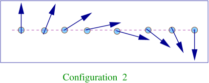
Figure 3: (Color online). Configuration $2$: A magnetic quantum wire with $N$ atomic sites where the magnetic moments are oriented in a wave like pattern. The moments in sites $1$ and $N$ are oppositely oriented.

Green’s function technique. Within the regime of coherent transport and for non-interacting systems this formalism is well applied.

The single particle Green’s function representing the full system for an electron with energy $E$ is defined as datta1 ; datta2 ,

$$\bf{G}=(\bf{E}-\bf{H})^{-1}$$ (5)

where,

$${\bf{E}}=(\epsilon+i\eta){\bf{I}}$$ (6)

In the above expression $i\eta$ is a small imaginary term added to the energy $\epsilon$ to make the Green’s function $\bf{G}$ non-hermitian.

Now, $\bf{H}$ and $\bf{G}$ representing the Hamiltonian and the Green’s function for the full system those can be partitioned in terms of different sub-Hamiltonians like datta1 ; datta2 ,

$$\bf{H}=\left(\begin{array}[]{ccc}\bf{H_{S}}&\bf{H_{SW}}&0\\ \bf{H_{SW}^{\dagger}}&\bf{H_{W}}&\bf{H_{WD}}\\ 0&\bf{H_{WD}^{\dagger}}&\bf{H_{D}}\\ \end{array}\right)$$ (7)

$$\bf{G}=\left(\begin{array}[]{ccc}\bf{G_{S}}&\bf{G_{SW}}&0\\ \bf{G_{SW}^{\dagger}}&\bf{G_{W}}&\bf{G_{WD}}\\ 0&\bf{G_{WD}^{\dagger}}&\bf{G_{D}}\\ \end{array}\right)$$ (8)

where, $\bf{H_{S}}$, $\bf{H_{W}}$ and $\bf{H_{D}}$ represent the Hamiltonians (in matrix form) for source, quantum wire and drain, respectively. $\bf{H_{SW}}$ and $\bf{H_{WD}}$ are the matrices for the Hamiltonians representing the wire-electrode coupling. Assuming that there is no direct coupling between the electrodes themselves, the corner elements of the matrices are zero. A similar definition goes for the Green’s function matrix ${\bf G}$ as well.

Our first goal is to determine $\bf{G_{W}}$ (Green’s function for the wire only) which defines all physical quantities of interest. Following Eq. (5) and using the block matrix form of $\bf{H}$ and $\bf{G}$ the form of $\bf{G_{W}}$ can be expressed as,

$$\bf{G_{W}}=(\bf{E}-\bf{H_{W}}-\bf{\Sigma_{S}}-\bf{\Sigma_{D}})^{-1}$$ (9)

where, $\bf{\Sigma_{S}}$ and $\bf{\Sigma_{D}}$ represent the contact self-energies introduced to incorporate the effects of semi-infinite electrodes coupled to the system, and, they are expressed by the relations datta1 ; datta2 ,

$$\bf{\Sigma_{S}} = \bf{H_{SW}^{{\dagger}}G_{S}H_{SW}}$$

$$\bf{\Sigma_{D}} = \bf{H_{WD}^{{\dagger}}G_{D}H_{WD}}$$ (10)

Thus, the form of self-energies are independent of the nano-structure itself through which transmission is studied and they completely describe the influence of electrodes attached to the system. Now, the transmission probability $(T_{\sigma\sigma^{\prime}})$ of an electron with energy $E$ is related to the Green’s function as,

$$T_{\sigma\sigma^{\prime}} = {\bf\Gamma}^{1}_{\bf{S}(\sigma\sigma)}{\bf G}^{1N}_{\bf{r}(\sigma\sigma^{\prime})}{\bf G}^{N1}_{\bf{a}(\sigma^{\prime}\sigma)}{\bf\Gamma}^{N}_{\bf{D}(\sigma^{\prime}\sigma^{\prime})}$$ (11)

$$= {\bf\Gamma}^{1}_{\bf{S}(\sigma\sigma)}|{\bf G}^{1N}_{(\sigma\sigma^{\prime})}|^{2}{\bf\Gamma}^{N}_{\bf{D}(\sigma^{\prime}\sigma^{\prime})}$$

where, ${\bf\Gamma}^{1}_{\bf{S}(\sigma\sigma)}=\langle 1\sigma|{\bf\Gamma_{S}}|1\sigma\rangle$ , ${\bf\Gamma}^{N}_{\bf{D}(\sigma^{\prime}\sigma^{\prime})}=\langle N\sigma^{\prime}|{\bf\Gamma_{D}}|N\sigma^{\prime}\rangle$ and ${\bf G}^{1N}_{\sigma\sigma^{\prime}}=\langle 1\sigma|{\bf G}|N\sigma^{\prime}\rangle$. Here, $\bf{G_{r}}$ and $\bf{G_{a}}$ are the retarded and advanced single particle Green’s functions (for the MQW only) for an electron with energy $E$. $\bf{\Gamma_{S}}$ and $\bf{{\Gamma_{D}}}$ are the coupling matrices, representing the coupling of the magnetic quantum wire to source and drain, respectively, and they are defined by the relation datta1 ; datta2 ,

$$\bf{\Gamma_{S(D)}}=i[\Sigma^{r}_{S(D)}-\Sigma^{a}_{S(D)}]$$ (12)

Here, $\bf{\Sigma^{r}_{S(D)}}$ and $\bf{\Sigma^{a}_{S(D)}}$ are the retarded and advanced self-energies, respectively, and they are conjugate to each other. It is shown in literature by Datta et al. that the self-energy can be expressed as a linear combination of a real and an imaginary part in the form,

$${\bf{\Sigma^{r}_{S(D)}}}={\bf\Lambda_{S(D)}}-i{\bf\Delta_{S(D)}}$$ (13)

The real part of self-energy describes the shift of the energy levels and the imaginary part corresponds to the broadening of the levels. The finite imaginary part appears due to incorporation of the semi-infinite electrodes having continuous energy spectrum. Therefore, the coupling matrices can easily be obtained from the self-energy expression and is expressed as,

$${\bf{\Gamma_{S(D)}}}=-2{\bf Im}{\bf{(\Sigma_{S(D)})}}$$ (14)

Considering linear transport regime, conductance $(g_{\sigma})$ is obtained using Landauer formula datta1 ; datta2 ,

$$g_{\sigma\sigma^{\prime}}=\frac{e^{2}}{h}T_{\sigma\sigma^{\prime}}$$ (15)

Knowing the transmission probability ($T_{\sigma\sigma^{\prime}}$) of an electron injected with spin $\sigma$ and transmitted with spin $\sigma^{\prime}$, the current ($I_{\sigma\sigma^{\prime}}$) through the system is obtained using Landauer-Büttiker formalism. It is written in the form datta1 ; datta2 ,

$$I_{\sigma\sigma^{\prime}}(V)=\frac{e}{h}\int\limits_{-\infty}^{+\infty}\left[f_{S}(E)-f_{D}(E)\right]T_{\sigma\sigma^{\prime}}(E)~{}dE$$ (16)

where, $f_{S(D)}=f(E-\mu_{S(D)})$ gives the Fermi distribution function of the two electrodes having chemical potentials $\mu_{S(D)}=E_{F}\pm eV/2$. $E_{F}$ is the equilibrium Fermi energy.

III Numerical results and discussion

We investigate various features of spin dependent transport through a magnetic quantum wire (MQW) for two different geometrical configurations depending on the orientations of the localized magnetic moments associated with each atomic site. In the first configuration, all the moments are aligned parallel to each other and initially they are chosen to be directed along $+Z$ direction, while in the second one the magnetic moments are oriented in a wave like pattern. All the results shown in the present work are obtained numerically. Therefore, we start analyzing the results by mentioning all the parameters those are used for numerical calculation. Our first assumption is that the two non-magnetic side-attached electrodes are made up of identical materials. The on-site energies in the wire ($\epsilon_{0}$) as well as in the leads ($\epsilon_{S(D)}$) are set as $0$. Hopping strength between the sites in the two electrodes is chosen as $t_{S(D)}=4$, whereas in the QW it is set as $t=3$. The equilibrium Fermi energy $E_{F}$ is fixed at $0$. Our unit system is simplified by choosing $h=c=e=1$. Energy scale is fixed in unit of $t$.

Throughout the analysis we address the basic features of spin dependent transport for two distinct regimes of electrode-to-MQW coupling. These regimes are described as follows. Case 1: Weak-coupling limit This limit is set by the criterion $t_{SW(WD)}<<t$. In this case, we choose the values as $t_{SW}=t_{WD}=0.5$.

Case 2: Strong-coupling limit This limit is described by the condition $t_{SW(WD)}\sim t$. In this regime we choose the values of hopping strengths as $t_{SW}=t_{WD}=2.5$.

III.1 Features of Spin Transport for Configuration $1$

III.1.1 Conductance-energy characteristics

First, we plot the conductance-energy characteristics for a magnetic quantum wire in which the moments are aligned along a preferred $Z$ direction according to the configuration $1$ (for instance see Fig. 2). As illustrative examples, in Fig. 4 we show the variation of conductances due to pure transmission of up and down spin electrons ($g_{\uparrow\uparrow}$ and $g_{\downarrow\downarrow}$) and spin flip transmission ($g_{\uparrow\downarrow}$ and $g_{\downarrow\uparrow}$) with respect to the injecting electron energy $E$ for a magnetic quantum wire considering $N=8$. It is observed that $g_{\uparrow\uparrow}$ and $g_{\downarrow\downarrow}$ exhibit sharp resonant peaks at some discrete energy values in the weak-coupling limit (green and blue curves

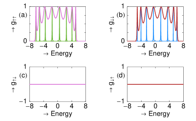
Figure 4: (Color online). $g$-$E$ characteristics for a magnetic quantum wire considering the system size $N=8$ where all moments are aligned along $+Z$ direction. The upper and lower panels describe the variations of $g_{\uparrow\uparrow}$, $g_{\downarrow\downarrow}$ and $g_{\uparrow\downarrow}$, $g_{\downarrow\uparrow}$, respectively. The green and blue curves represent the results in the weak-coupling limit, while the curves in pink and red depict the results in the strong coupling limits, respectively. Conductances are measured in unit of $e^{2}/h$, while the energy is measured in unit of $t$.

of Figs. 4(a) and (b)), whereas the peaks acquire some broadening in the limit of strong-coupling (pink and red curves of Figs. 4(a) and (b)). The broadening of conductance peaks with the enhancement in coupling strength is quantified by the imaginary parts $\bf{\Delta_{S}}$ and $\bf{\Delta_{D}}$ of the self-energy matrices $\bf{\Sigma_{S}}$ and $\bf{\Sigma_{D}}$ which are incorporated in the conductance expression via the coupling matrices datta1 ; datta2 . All these resonant peaks are associated with the energy eigenvalues of the magnetic quantum wire. Therefore, it is manifested that the conductance-energy spectrum reveals the feature of energy spectrum of the wire completely. One interesting feature to be noted here is that, variation of $g_{\uparrow\uparrow}$ and $g_{\downarrow\downarrow}$ with energy ($E$) are exactly mirror symmetric about $E=0$ as we set $\epsilon_{0}=0$. For any other non-zero value of $\epsilon_{0}$, up and down spin channels get splitted but the conductance spectra does not remain mirror symmetric anymore.

On the other hand, in this particular configuration the conductance by spin flipping becomes exactly zero for the entire energy region as seen from Figs. 4(c) and (d), where the curves for the weak- and strong-coupling limits overlap to each other. The reason of zero spin flipping is explained as follows. Occurrence of spin flipping is governed by the term $\vec{h}.\vec{\sigma}$ in the Hamiltonian (see Eq. (2)), where $\vec{\sigma}$ stands for the Pauli spin matrix having components $\sigma_{x}$, $\sigma_{y}$ and $\sigma_{z}$ for the injecting electron and $h$ being the localized magnetic moments associated with each magnetic site in the quantum wire (QW). Spin flipping is mathematically expressed by the operation of raising ($\sigma_{+}=\sigma_{x}+i\sigma_{y}$) and lowering ($\sigma_{-}=\sigma_{x}-i\sigma_{y}$) operators. For the local

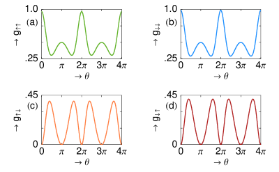
Figure 5: (Color online). Variation of conductances with polar angle $\theta$ for a magnetic quantum wire considering $N=16$ and $E=3.2$ in the limit of strong wire-electrode coupling strength. The upper and lower panels correspond to the cases of $g_{\uparrow\uparrow}$, $g_{\downarrow\downarrow}$ and $g_{\uparrow\downarrow}$, $g_{\downarrow\uparrow}$, respectively.

magnetic moments oriented along $\pm$ $Z$ axis i.e., for $\theta=0~{}\mbox{and}~{}\pi$, $\vec{h}.\vec{\sigma}$ ($=h_{x}\sigma_{x}+h_{y}\sigma_{y}+h_{z}\sigma_{z}$) becomes equal to $h_{z}\sigma_{z}$. Accordingly, the Hamiltonian does not contain $\sigma_{x}$ and $\sigma_{y}$ and so as $\sigma_{+}$ and $\sigma_{-}$, which provides zero flipping for up or down orientation of magnetic moments.

III.1.2 Variation of conductance with polar angle $\theta$

To reveal the effect of orientation of local magnetic moments on spin dependent transport, in Fig. 5 we plot the variation of conductances ($g_{\uparrow\uparrow}$, $g_{\downarrow\downarrow}$ and $g_{\uparrow\downarrow}$, $g_{\downarrow\uparrow}$) with angle $\theta$ made by the magnetic moments with the preferred $+Z$ direction. It is evident from this figure that the conductances ($g_{\uparrow\uparrow}$, $g_{\downarrow\downarrow}$, $g_{\uparrow\downarrow}$ and $g_{\downarrow\uparrow}$) exhibit $2\pi$ periodicity as a function of $\theta$ with reflection symmetry at $\theta=\pi$.

Rotation of magnetic moments through an angle $2\pi$ maps themselves into their initial positions. So $2\pi$ periodicity in the variation of conductances with $\theta$ is expected. Reflection symmetry about $\theta=\pi$ is equivalent to having a symmetry point at $\theta=0$, which means rotation of magnetic moments from up to down direction is independent of the sense of rotation.

III.1.3 Current-voltage characteristics

All the essential features of spin transport described earlier will be more transparent from our current-voltage characteristics. Current through the MQW is computed by integrating over the transmission curve following Landauer-Büttiker formalism. Transmission probability varies in an

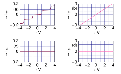
Figure 6: (Color online). $I_{\uparrow\uparrow}$ and $I_{\uparrow\downarrow}$ as a function of applied bias voltage $V$ for a magnetic quantum wire with $N=8$, where all magnetic moments are aligned along $+Z$ direction. The left and right columns correspond to the cases of weak and strong wire to electrode coupling limits, respectively. $I$ and $V$ are measured in units of $te/h$ and $t/e$, respectively.

exactly identical way to that of the conductance spectrum apart from a scale factor $e^{2}/h$ (which is equal to $1$ in our chosen unit system) according to Eq. (15). The current $I_{\uparrow\uparrow}$ shows staircase like pattern (Fig. 6(a)) due to the presence of sharp, discrete resonant peaks in conductance-energy spectrum in the limit of weak-coupling. With the increase in applied bias voltage $V$, the difference in chemical potentials of the two electrodes ($\mu_{S}-\mu_{D}$) increases, allowing more number of energy levels to fall in that range, and accordingly, more energy channels are accessible to the injected electrons to pass through the magnetic quantum wire from source to drain. Incorporation of a single discrete energy level i.e., a discrete quantized conduction channel, between the range ($\mu_{S}-\mu_{D}$) provides a jump in the $I$-$V$ characteristics. Contribution to the current $I_{\uparrow\downarrow}$ due to spin flipping is zero (Fig. 6(c)) as the spin flip transmission probability is zero for this configuration $1$.

In the limit of strong wire-electrode coupling, due to the broadening of conductance peaks current $I_{\uparrow\uparrow}$ shows nearly linear variation (Fig. 6(b)) as a function of applied bias voltage

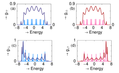
Figure 7: (Color online). $g$-$E$ characteristics for a magnetic quantum wire considering the system size $N=8$ where the magnetic moments are aligned according to configuration $2$ (Fig. 3). The upper and lower panels describe the variations of $g_{\uparrow\uparrow}$, $g_{\downarrow\downarrow}$ and $g_{\uparrow\downarrow}$, $g_{\downarrow\uparrow}$, respectively. The blue and pink curves represent the results in the weak-coupling limit, while the deep blue and deep red lines correspond to the results in the strong-coupling limit.

$V$ and acquires much higher amplitude compared to the weak-coupling limit. Enhancement in coupling strength does not change spin flip transmission probability, and hence, $I_{\uparrow\downarrow}$ shows zero value for the entire range of the bias voltage $V$ (Fig. 6(d)). Current due to down spin shows the same kind of variation with applied bias voltage. So this has not been shown in the above figure.

III.2 Features of Spin Transport for Configuration $2$

Following the above description of spin dependent transport now we concentrate on a magnetic quantum wire in which the moments are aligned in a wave like pattern as illustrated in Fig. 3.

III.2.1 Conductance-energy characteristics

As representative examples, in Fig. 7 we plot the variation of conductances due to pure spin transmission ($g_{\uparrow\uparrow}$ and $g_{\downarrow\downarrow}$) and spin flip transmission ($g_{\uparrow\downarrow}$ and $g_{\downarrow\uparrow}$) for a MQW considering $N=8$. Variation of $g_{\uparrow\uparrow}$ and $g_{\downarrow\downarrow}$ exhibits sharp peaks at some discrete energy values in the weak-coupling limit (blue and pink curves of Figs. 7(a) and (b)), while in the limit of strong-coupling they achieve substantial broadening with larger amplitude

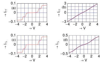
Figure 8: (Color online). $I_{\uparrow\uparrow}$ and $I_{\uparrow\downarrow}$ as a function of applied bias voltage $V$ for a magnetic quantum wire with $N=8$, where the magnetic moments are aligned according to the configuration $2$ (Fig. 3). The left and right columns correspond to the cases of weak and strong wire to electrode coupling strengths, respectively.

(deep blue and deep red curves of Figs. 7(a) and (b)). This broadening effect is clearly understood from our previous discussion. But for this type of configuration i.e., where the orientation of each magnetic moment is increased gradually with respect to $+Z$ axis along the length of the quantum wire, conductance amplitude due to pure spin transmission ($g_{\uparrow\uparrow}$ and $g_{\downarrow\downarrow}$) in the limit of strong-coupling is sufficiently higher than that of the weak-coupling case.

For this typical configuration, non-zero conductance due to spin flip transmission is obtained as given in Figs. 7(c) and (d). Here, the magnitude of spin flip conductances are comparable in both the two coupling limits. As in the previous case, conductance-energy spectrum due to up and down spins are mirror symmetric to each other across the energy $E=0$, both for pure spin transmission as well as spin flip transmission, since we set $\epsilon_{0}=0$ in this case also.

III.2.2 Current-voltage characteristics

In Fig. 8 we show the variations of spin dependent currents $I_{\uparrow\uparrow}$ and $I_{\uparrow\downarrow}$ as a function of applied bias voltage $V$ for a magnetic quantum wire considering the system size $N=8$ in both the two coupling limits. All the basic features of currents are same as we observe in the case of configuration $1$ e.g., step-like behavior in the weak-coupling limit and almost linear variation with larger amplitude in the limit of strong-coupling. But the notable signatures for this configuration are non-zero current due to spin flipping $I_{\uparrow\downarrow}$, and comparable amplitude of $I_{\uparrow\uparrow}$ and $I_{\uparrow\downarrow}$ in the weak-coupling limit for this system size. Here also the down spin current shows the same nature of variation with the applied bias voltage and correspondingly we do not plot it.

III.2.3 Variation of conductance with system size $N$

At the end, in Fig. 9 we present the variations of $g_{\uparrow\uparrow}$ and $g_{\uparrow\downarrow}$ with system size $N$ in the limit of strong-coupling. The conductances are calculated at the typical energy $E=1.5$. For such configuration $g_{\uparrow\downarrow}$ increases gradually with system size $N$, while $g_{\uparrow\uparrow}$ decreases with the rise of $N$. For this configuration, the magnetic moments are oriented sequentially from $0$ to $\pi$ and from earlier discussion it is evident

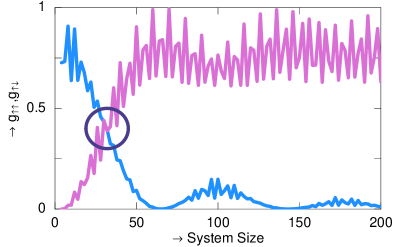
Figure 9: (Color online). Variations of $g_{\uparrow\uparrow}$ and $g_{\uparrow\downarrow}$ with system size $N$ for the typical energy $E=1.5$ in the limit of strong wire-electrode coupling. The blue and pink curves correspond to the features of $g_{\uparrow\uparrow}$ and $g_{\uparrow\downarrow}$, respectively.

that spin flip does occur when the magnetic moments are oriented at an angle $\theta$ with respect to the preferred $+Z$ direction. Hence, for the configuration $2$, $g_{\uparrow\downarrow}$ increases with system size due to large number of sequential spin flip scattering and after a critical system size marked by the violet circle in Fig. 9, spin flip transmission dominates significantly over pure spin transmission. The critical size decreases with increase in injecting electron energy which is not shown in Fig. 9. In case of down spin propagation similar features of system size dependence is observed and we do not show this.

IV Closing remarks

In a nutshell, in the present work we study spin dependent transport through a magnetic quantum wire (MQW) using single particle Green’s function technique. We have adopted a discrete lattice model in tight-binding framework to illustrate the system which is simply an array of identical magnetic atomic sites. In our theoretical study two different geometrical configurations of the MQW depending on the orientation of the magnetic moments associated with each magnetic site. In the first configuration, all the moments are aligned at an equal angle with respect to the $+Z$ axis, while in the second one the moments are sequentially oriented from angle $0$ to $\pi$ relative to the $+Z$ direction. Orientation of the magnetic moments can be changed by applying an external magnetic field.

We investigated conductance-energy ($g$-$E$) and current-voltage ($I$-$V$) characteristics for both the two configurations mentioned above. Non-zero spin flip conductances ($g_{\uparrow\downarrow}$ and $g_{\uparrow\downarrow}$) are obtained for configuration $2$, whereas it is zero for up or down orientation of localized moments as illustrated in configuration $1$. In addition to these we observed the dependence of conductances on polar angle $\theta$ for configuration $1$, showing $2\pi$ periodicity. In the last figure, we have plotted the variations of $g_{\uparrow\uparrow}$ and $g_{\uparrow\downarrow}$ with the system size $N$ for typical electron energy $E=1.5$ in the limit of strong wire-electrode coupling, which is the most interesting part of our theoretical study. It clearly demonstrates that after a certain system size spin flip transmission dominates significantly over the pure spin transmission. For a sufficiently large system, spin inversion takes place most prominently which can be utilized for fabricating spin based nano devices.

In the present work we have calculated all these results by ignoring the effects of temperature, spin-orbit interaction, electron-electron correlation, electron-phonon interaction, disorder, etc. Here, we set the temperature at $0$K, but the basic features will not change significantly even in non-zero finite (low) temperature region as long as thermal energy ($k_{B}T$) is less than the average energy spacing of the energy levels of the magnetic quantum wire. In this model it is also assumed that the two side-attached non-magnetic electrodes have negligible resistance.

All these predicted results using such simple geometric configurations may be useful in designing a spin based nano devices.

References

- (1) J. Chen, M. A. Reed, A. M. Rawlett, and J. M. Tour, Science 286, 1550 (1999).
- (2) P. Ball, Nature (London) 404, 918 (2000).
- (3) S. A. Wolf et al., Science 294, 1488 (2001).
- (4) G. Prinz, Science 282, 1660 (1998).
- (5) G. Prinz, Phys. Today 48, 58 (1995).
- (6) M. N. Baibich, J. M. Broto, A. Fert, F. N. Van Dau, F. Petroff, P. Etienne, G. Creuzet, A. Friederich, and J. Chazelas, Phys. Rev. Lett. 61, 2472 (1998).
- (7) Rokhinson et al., Phys. Rev. Lett. 93, 146601 (2004).
- (8) Schönenberger et al., Nature Phys. 1, 99 (2005).
- (9) Tombros et al., Nature. 448, 571 (2007).
- (10) I. A. Shelykh, N. T. Bagraev, N. G. Galkin, and L. E. Klyanchkin, Phys. Rev. B 71, 113311 (2005).
- (11) H. W. Wu, J. Zhou, and Q. W. Shi, Appl. Phys. Lett. 85, 1012 (2004).
- (12) M. Dey, S. K. Maiti, and S. N. Karmakar, Phys. Lett. A 374, 1522 (2010).
- (13) D. Frustaglia, M. Hentschel, and K. Richter, Phys. Rev. Lett. 87, 256602 (2001).
- (14) R. Ionicioiu and I. D’Amico, Phys. Rev. B 67, 041307(R) (2003).
- (15) A. A. Shokri, M. Mardaani, and K. Esfarjani, Physica E 27, 325 (2005).
- (16) A. A. Shokri, M. Mardaani, and K. Esfarjani, Physica E 27, 325 (2005).
- (17) A. A. Shokri and M. Mardaani, Solid State Commun. 137, 53 (2006).
- (18) M. Mardaani and A. A. Shokri, Chem. Phys. 324, 541 (2006).
- (19) A. A. Shokri and A. Daemi, Eur. Phys. J. B 69, 245 (2009).
- (20) A. A. Shokri and A. Saffarzadeh, J. Phys.: Condens. Matter 16, 4455 (2004).
- (21) S. K. Maiti, Phys. Lett. A 373, 4470 (2009).
- (22) S. K. Maiti, J. Phys. Soc. Jpn. 78, 114602 (2009).
- (23) S. Datta, Electronic transport in mesoscopic systems, Cambridge University Press, Cambridge (1997).
- (24) S. Datta, Quantum Transport: Atom to Transistor, Cambridge University Press, Cambridge (2005).
- (25) R. Landauer, Phys. Lett. A 85, 91 (1986).
- (26) R. Landauer, IBM J. Res. Dev. 32, 306 (1988).
- (27) M. Büttiker, IBM J. Res. Dev. 32, 317 (1988).