Scheduling in Wireless Networks under Uncertainties: A Greedy Primal-Dual Approach

Abstract

This paper proposes a dynamic primal-dual type algorithm to solve the optimal scheduling problem in wireless networks subject to uncertain parameters, which are generated by stochastic network processes such as random packet arrivals, channel fading, and node mobilities. The algorithm is a generalization of the well-known max-weight scheduling algorithm proposed by Tassiulas et al., where only queue length information is used for computing the schedules when the arrival rates are uncertain. Using the technique of fluid limits, sample path convergence of the algorithm to an arbitrarily close to optimal solution is proved, under the assumption that the Strong Law of Large Numbers (SLLN) applies to the random processes which generate the uncertain parameters. The performance of the algorithm is further verified by simulation results. The method may potentially be applied to other applications where dynamic algorithms for convex problems with uncertain parameters are needed.

I Introduction

Scheduling in wireless networks involves efficiently allocating network resources among competing network users in the presence of uncertainties. These uncertainties may be either due to unexpected events, such as link failures, or due to intricate cross-layer interactions in wireless networks. For example, the packet arrival rates may be unknown (e.g., [1], [2]), which depend on upper layer dynamics such as routing and congestion control protocols. As another example, the wireless channel statistics may be also unknown (e.g., [2]), since they depend on complex network events such as channel fading, power control and node mobilities.

In the presence of such uncertain parameters, it may no longer be optimal to use the static allocation approach (e.g., [3]), which produces periodic schedules by solving a static underlying convex optimization problem (which usually has exponential size) with estimated uncertain parameters. In particular, if these uncertain parameters are slowly converging, or time varying, the estimated parameters may fail to track the changes in their true value, which often leads to suboptimal schedules. Further, it may be impractical to estimate the uncertain parameters for large wireless networks, as the number of the parameters may grow fast (e.g., exponentially) with the size of the network. For a simple illustration, consider a wireless network with $n$ links, such that each link randomly switches on or off after certain random number of time slots. In such case, a complete specification of the network topology probabilities may require as large as $2^{n}-1$ parameters, which quickly becomes impossible to estimate as $n$ grows.

On the other hand, online algorithms (such as [1], [2], [4], [6], [7]) are more robust to the changes to the uncertain parameters (such as arrival rates), since they use queue length (which can also be interpreted as prices [9], [10]) information for scheduling in each time slot. For example, it has been shown that [4] such algorithms can achieve network stability even if the “instantaneous rates” of the traffic vary arbitrarily inside the network capacity region. Further, compared to the estimation based approach, these online algorithms may be more scalable to the network size, in the sense that the dimension of the queue length vector corresponds to the number of constraints (such as rate constraint for each link), which usually grows slowly, whereas the number of uncertain parameters can grow very fast (e.g., exponentially).

In this paper we solve a general class of optimal wireless network scheduling problems with uncertain parameters, whose underlying static problem is described by the convex optimization problem OPT in Section II. Essentially, we require that the structures of the convex objective functions and convex constraint functions are known, except the values of the uncertain parameters. These parameters will be generated by certain stochastic processes and observed by the network gradually over time slots. We propose a greedy primal-dual dynamic algorithm (Algorithm 1 in Section III) to achieve the optimal scheduling asymptotically. Using the novel technique of fluid limits [12], optimality can be guaranteed under the assumption that all the network processes generating the uncertain parameters satisfy SLLN (see details in Section II). Note that this assumption is quite mild, since we can guarantee optimality as long as these processes converge, no matter how slowly the convergence happen. Thus, intuitively, our algorithm can automatically track the convergence of these processes and correct the mistakes which are made within any finite time history.

Our algorithm is a generalization of the well-known max-weight algorithm [1], which was shown to be throughput optimal for i.i.d arrival processes. Our algorithm is related to, but different from the utility-optimal scheduling algorithm by Neely [2], which achieves the optimal scheduling by cleverly transforming the problem into optimizing the time-average of the utility (and constraint) functions, to which a dual-type algorithm applies. Our algorithm is also different from the primal-dual algorithm by Neely [5] since we use a scaled queue length (by $1/t$) in the scheduling, which corresponds to the approximated gradient. Stolyar [6] also proposed a primal-dual type scheduling algorithm, and proved its optimality using a fluid limit obtained from a different scaling. Since the fluid scaling in [6] is taken over different systems, it is hard to relate the optimality in the fluid limits to the one in the original system. Finally, our algorithm can be used as a MAC layer solution for the general framework of cross-layer optimization problem (e.g., [4], [7], [8], [10]) for wireless networks.

The organization of the following sections is as follows: In Section II we describe the queueing network model as well as the optimization problem OPT, and in Section III we describe the scheduling algorithm. Section IV proves the optimality of the algorithm, Section V illustrate the algorithm performance in simulation, and finally Section VI concludes this paper.

II Network Model and Problem Formulation

In this section we describe the queueing network and propose the optimization problem OPT. We first introduce the queueing network model.

II-A Queueing Network

We consider the scheduling problem at the medium access (MAC) layer of a multi-hop wireless network, where the network is modeled as a set of $n$ links. We assume a time-slotted network model, and in each time slot $t$, the network is in one of the following states: $\mathcal{M}\triangleq\{1,2,\ldots,M\}$. The network state can be used to model network topology, channel fading, and user mobility, etc. We further assume that these network states can be measured by the user nodes, which are assumed to be equipped with channel monitoring devices. We associate each network state $m\in\mathcal{M}$ with a finite set of resource allocation modes $\Xi^{(m)}=\{\xi^{(m)}_{1},\xi^{(m)}_{2},\ldots\}$, where each mode $\xi^{(m)}_{k}\in\Xi^{(m)}$ corresponds to a configuration of network resource allocation, such as carrier and frequency selection in OFDM systems, spreading codes choice in CDMA systems and time slots assignment in TDMA systems.

Denote $\boldsymbol{y}$ as the uncertain parameters, which are generated by the stochastic process $\boldsymbol{Y}(t)$, which is a cumulative vector process whose time average converges to $\boldsymbol{y}$. Specifically, the assumptions on $\boldsymbol{Y}(t)$ are: 1) it is subject to SLLN, i.e., with probability 1 (w.p.1),

$$\lim_{t\rightarrow\infty}\boldsymbol{Y}(t)/t=\boldsymbol{y}$$ (1)

and 2) it has uniformly bounded increment in each time slot:

$$\|\boldsymbol{Y}(t)-\boldsymbol{Y}(t-1)\|\leq Y_{\max},\forall t>0$$ (2)

where $Y_{\max}>0$ is a finite constant. For specific examples, consider the cumulative network state process $M_{m}(t)$:

$$S_{m}(t)=\sum_{\tau=1}^{t}\mathbbold{1}_{\{m(\tau)=m\}}$$ (3)

where $m(t)$ is the network state at time slot $t$, and $\mathbbold{1}_{\{\cdot\}}$ is the indicator function, i.e., $\mathbbold{1}_{\{\text{true}\}}=1$ and $\mathbbold{1}_{\{\text{false}\}}=0$. Thus, SLLN implies that w.p.1,

$$\lim_{t\rightarrow\infty}{1\over t}S_{m}(t)=\lim_{t\rightarrow\infty}{1\over t}\sum_{\tau=1}^{t}\mathbbold{1}_{\{m(\tau)=m\}}=\pi^{(m)},\ \forall m\in\mathcal{M}$$

As another example, consider the external packet arrival process $\boldsymbol{A}(t)$, which is a $n\times 1$ vector representing the cumulative external packet arrivals during the first $t$ time slots. Similarly, SLLN implies that w.p.1,

$$\lim_{t\rightarrow\infty}{\boldsymbol{A}}(t)/t={\boldsymbol{a}},\ \textrm{w.p.1}$$ (4)

Further, we require that the maximum packet arrivals in any time slot are uniformly bounded:

$$\|\boldsymbol{A}(t)-\boldsymbol{A}(t-1)\|\leq A_{\max},\ \forall t>0$$ (5)

where $A_{\max}>0$ is a finite constant.

We finally describe the queueing system model. The queuing dynamics of the network is modeled as follows:

$${\boldsymbol{Q}}(t)={\boldsymbol{Q}}(0)+{\boldsymbol{A}}(t)-R(m(t)){\boldsymbol{D}}(t)$$ (6)

where ${\boldsymbol{Q}}(t)$ is the queue length vector at time slot $t$, and $R(m(t))$ is the $n\times n$ routing matrix, such that $R_{ii}(m(t))=1$, and $R_{ij}(m(t))=-1$ only if link $i$ serves as the next hop for link $j$ at time slot $t$, as specified by certain routing protocols, otherwise $R_{ij}(m(t))=0$. Note that the routing matrix $R(m(t))$ is a function of the network state, and therefore SLLN implies

$$\lim_{t\rightarrow\infty}{1\over t}\sum_{\tau=1}^{t}R(m(\tau))=\sum_{m\in\mathcal{M}}\pi^{(m)}R(m)$$ (7)

${\boldsymbol{D}}(t)$ is a $n\times 1$ vector representing the cumulative packet departures during the first $t$ time slots, which are determined by the resource allocation modes as specified by the scheduler in each time slot. Specifically, at each time slot $t$ with network state $m$, if the scheduler chooses a resource allocation mode $\xi_{k}^{(m)}$, there is an associated departure vector $\boldsymbol{G}^{(m)}_{k}$, whose each entry ${G}^{(m)}_{ki}$ corresponds to the number of packets transmitted successfully by link $i$. Note that the choice of resource allocation mode $\xi_{k}^{(m)}$ is subject to the constraint that $\boldsymbol{Q}(t)-\boldsymbol{G}^{(m)}_{k}\succeq\boldsymbol{0}$, so that the queue lengths never become negative. Note that this constraint can be easily satisfied in general systems. For example, if the allocation mode $\xi_{k}^{(m)}$ corresponds to independent sets of the interference graph (see, for example, [7]), one can simply transmit the subset of links with nonempty queues, which are still independent. In a compact form, we can express the departure process as

$${\boldsymbol{D}}(t)=\sum_{m\in{\mathcal{M}}}G^{(m)}{\boldsymbol{T}}^{(m)}(t),$$ (8)

where $G^{(m)}$ is a matrix whose columns are $\boldsymbol{G}^{(m)}_{k}$, and ${\boldsymbol{T}}^{(m)}(t)$ is a vector whose each entry ${T}^{(m)}_{k}(t)$ corresponds to the number of time slots that resource allocation mode $\xi^{(m)}_{k}$ is chosen during the first $t$ time slots.

A basic requirement on the scheduler is that it should achieve rate stability [12], i.e.,

$$\lim_{t\rightarrow\infty}\boldsymbol{D}(t)/t=\boldsymbol{a}$$ (9)

so that the departure rate of each link is equal to the arrival rate, as required by the underlying static optimization problem OPT, which we formulate in the next subsection.

II-B Optimization Problem

In this section we introduce the optimization problem OPT, which is implicitly solved by the optimal schedulers. The problem OPT is as follows OPT:

$$\textsf{OPT: }\min_{{\boldsymbol{x}}} f({\boldsymbol{x}};{\boldsymbol{y}})$$ (10)

s.t. $$\boldsymbol{h}({\boldsymbol{x}};{\boldsymbol{y}})\preceq{\boldsymbol{0}}$$ (12)

$${\boldsymbol{x}}^{(m)}\succeq 0,\ {\boldsymbol{1}}^{T}{\boldsymbol{x}}^{(m)}=1,\ \forall m\in\mathcal{M}$$

In the above formulation, $\boldsymbol{x}^{(m)}$ as a resource allocation vector when the network state is $m$. That is, each entry $x_{k}^{(m)}$ is the asymptotic time fraction (assuming the limit exists for now) that resource allocation mode $\xi^{(m)}_{k}$ is chosen, during the time slots where the network state is $m$. Thus, $\boldsymbol{x}^{(m)}$ is subject to the simplex constraint (12). $\boldsymbol{x}=(\boldsymbol{x}^{(1)},\boldsymbol{x}^{(2)},\ldots,\boldsymbol{x}^{(M)})$ is a big vector representing the total resource allocation vector as specified by the scheduler. $f({\boldsymbol{x}};{\boldsymbol{y}})$ is a general convex cost function of variable $\boldsymbol{x}$, and $\boldsymbol{h}({\boldsymbol{x}};{\boldsymbol{y}})$ is a vector of general convex constraint functions of variable $\boldsymbol{x}$. The additional parameter ${\boldsymbol{y}}$ represents the uncertain parameters, which is valid under the assumption that the corresponding processes are subject to SLLN. Finally, we assume that both $f({\boldsymbol{x}};{\boldsymbol{y}})$ and $h({\boldsymbol{x}};{\boldsymbol{y}})$ are continuously differentiable as functions of variables $(\boldsymbol{x},\boldsymbol{y})$.

The formulation of OPT is quite general, which can be used to model various applications in the literature. For example, if we want to minimize the total transmission power, we can choose $\boldsymbol{y}=(\boldsymbol{\pi},\boldsymbol{p})$, and choose the cost function as follows

$$f({\boldsymbol{x}};{\boldsymbol{y}})=\sum_{m\in\mathcal{M}}\pi^{(m)}\boldsymbol{p}^{(m)T}\boldsymbol{x}^{(m)}$$ (13)

where $\pi^{(m)}$ is the time fraction that the network state is $m$, and $\boldsymbol{p}^{(m)}$ is a power vector where each entry $p^{(m)}_{k}$ corresponds to the power consumption when resource allocation mode $\xi^{(m)}_{k}$ is chosen at network state $m$. Thus, the cost function in (13) can be interpreted as the average power consumption by the scheduler. Note that we can also encode the power constraint into $\boldsymbol{h}({\boldsymbol{x}},{\boldsymbol{y}})$ by choosing $\boldsymbol{y}=(\boldsymbol{\pi},\boldsymbol{p})$ and then choosing

$$\boldsymbol{h}(\boldsymbol{x};\boldsymbol{y})=\sum_{m\in\mathcal{M}}\pi^{(m)}P^{{(m)}}\boldsymbol{x}^{(m)}-\boldsymbol{p}$$ (14)

where $P^{{(m)}}$ is a diagonal matrix where each diagonal entry $P^{(m)}_{kk}$ corresponds to the power consumption when resource allocation mode $\xi_{k}^{(m)}$ is chosen when the network state is $m$, and $\boldsymbol{p}$ is the power constraint vector. In this case, (14) is equivalent to requiring a constraint of $\boldsymbol{p}$ on the average transmission power. In order to encode the network stability constraint, we can choose $\boldsymbol{y}=(\boldsymbol{\pi},\boldsymbol{a})$ and then choose

$$\boldsymbol{h}({\boldsymbol{x};\boldsymbol{y}})=\boldsymbol{a}-\sum_{m\in\mathcal{M}}\pi^{(m)}R(m)G^{{(m)}}\boldsymbol{x}^{(m)}$$ (15)

Thus, (15) requires that the average external and internal arrivals should be less than the average departures, in which case the network is rate stable.

III Scheduling Algorithm

In this section we will describe the algorithm to solve OPT. As a standard approach in solving constrained convex optimization problems [11], we transform OPT into another static “penalized” problem, PEN, to which our scheduling algorithm can directly apply. Based on this, we then introduce the scheduling algorithm which solves PEN and, therefore, also solves OPT.

III-A Transformed Problem

Assuming that OPT is strictly feasible, we first change the constraints in (12) as follows

$$\boldsymbol{h}({\boldsymbol{x}};\boldsymbol{y})+{\boldsymbol{z}}={\boldsymbol{0}},\ \epsilon{\boldsymbol{1}}\preceq{\boldsymbol{z}}\preceq{z}_{\max}\boldsymbol{1}$$ (16)

where $\epsilon>0$ is a small scalar, and ${z}_{\max}>0$ is a sufficiently large constant such that the inequality and equality constraints are equivalent. Denote $f^{\star}_{\epsilon}$ as the optimal cost when the constraint is changed to (16). Thus, the optimal value of OPT is $f^{\star}_{0}$. We have the following sensitivity lemma stating that $f^{\star}_{\epsilon}$ is a good approximation of $f^{\star}_{0}$ with sufficiently small $\epsilon$.

Lemma 1 ([11])

Denote $\boldsymbol{\lambda}_{0}$ and $\boldsymbol{\lambda}_{\epsilon}$ as two Lagrangian multipliers for $f^{\star}_{0}$ and $f^{\star}_{\epsilon}$, respectively. We have

$$|f^{\star}_{0}-f^{\star}_{\epsilon}|\leq\epsilon\max(\|\boldsymbol{\lambda}_{\epsilon}\|_{1},\|\boldsymbol{\lambda}_{0}\|_{1})$$ (17)

We next define the transformed problem as follows:

$$\textsf{PEN: }\min_{{\boldsymbol{x},\boldsymbol{z}}} g({\boldsymbol{x}},{\boldsymbol{z}};\boldsymbol{y})=f({\boldsymbol{x}};\boldsymbol{y})+\beta p({\boldsymbol{x}},{\boldsymbol{z}};\boldsymbol{y})$$

s.t. $$\epsilon{\boldsymbol{1}}\preceq{\boldsymbol{z}}\preceq{z}_{\max}\boldsymbol{1}$$

$${\boldsymbol{x}}^{(m)}\succeq 0,\ {\boldsymbol{1}}^{T}{\boldsymbol{x}}^{(m)}=1,\ \forall m\in\mathcal{M}$$

where $\beta$ is a large constant to control approximation accuracy, and $p({\boldsymbol{x}},{\boldsymbol{z}};\boldsymbol{y})$ corresponds to the penalty term, which corresponds to various standard penalty functions [11], e.g.,

$$p({\boldsymbol{x}},{\boldsymbol{z}};\boldsymbol{y})={1\over\alpha}\|\boldsymbol{h}({\boldsymbol{x}};\boldsymbol{y})+{\boldsymbol{z}}\|^{\alpha}$$ (18)

for $\alpha>1$. In particular, the standard Lyapunov drift analysis (e.g., [1], [2], [4], [7]) corresponds to the case $\alpha=2$.

Denote $({\boldsymbol{x}}^{\star}_{\textsf{p}},{\boldsymbol{z}}^{\star}_{\textsf{p}})$ as a solution of PEN. We have the following result holds:

Lemma 2

$f({\boldsymbol{x}}^{\star}_{\textsf{p}};\boldsymbol{y})\leq f^{\star}_{\epsilon}$.

Proof:

Denote $(\boldsymbol{x}^{\star}_{\textsf{o}},\boldsymbol{z}^{\star}_{\textsf{o}})$ as a solution of OPT with constraint in (12) replaced by (16). We have

$$f({\boldsymbol{x}}^{\star}_{\textsf{p}};\boldsymbol{y}) \leq f({\boldsymbol{x}}^{\star}_{\textsf{p}};\boldsymbol{y})+\beta p({\boldsymbol{x}}^{\star}_{\textsf{p}},{\boldsymbol{z}}^{\star}_{\textsf{p}};\boldsymbol{y})$$

$$\stackrel{{\scriptstyle(a)}}{{\leq}} f({\boldsymbol{x}}^{\star}_{\textsf{o}};\boldsymbol{y})+\beta p({\boldsymbol{x}}^{\star}_{\textsf{o}},{\boldsymbol{z}}^{\star}_{\textsf{o}};\boldsymbol{y})$$

$$\stackrel{{\scriptstyle(b)}}{{=}} f^{\star}_{\epsilon}$$

where $(a)$ is because $(\boldsymbol{x}^{\star}_{\textsf{p}},\boldsymbol{z}^{\star}_{\textsf{p}})$ solves PEN, and $(b)$ is because $(\boldsymbol{x}^{\star}_{\textsf{o}},\boldsymbol{z}^{\star}_{\textsf{o}})$ satisfy the constraint (16). Thus, the claim holds. ∎

In the following we will focus on solving PEN, since Lemma 1 and Lemma 2 guarantee that PEN achieve an objective function value which is arbitrarily close to the optimal in OPT. We next describe the scheduling algorithm.

III-B Algorithm Description

The problems OPT and PEN are static. On the other hand, the network is dynamic, and must be described by time series. Therefore, before describing the algorithm, we need to define dynamic counterparts of the static variables $\boldsymbol{x},\boldsymbol{y}$ and $\boldsymbol{z}$. We first define empirical resource allocation variable

$${\boldsymbol{x}}^{(m)}(t)={{\boldsymbol{T}}^{(m)}(t)\over{\boldsymbol{1}}^{T}{\boldsymbol{T}}^{(m)}(t)},\ \forall m\in\mathcal{M}$$ (19)

i.e., each entry ${x}_{k}^{(m)}(t)$ corresponds to the time fraction that resource allocation mode ${\xi}^{(m)}_{k}$ is chosen during the first $t$ time slots, when the network state is $m$. Note that we have

$${\boldsymbol{x}}^{(m)}(t)\succeq 0,\ {\boldsymbol{1}}^{T}{\boldsymbol{x}}^{(m)}(t)=1,\ \forall m\in\mathcal{M}$$ (20)

Thus, ${\boldsymbol{x}}^{(m)}(t)$ can be interpreted as the empirical value of ${\boldsymbol{x}}^{(m)}$ which is defined in PEN. Similarly, we denote the empirical value of the uncertain parameter $\boldsymbol{y}$ as

$$\boldsymbol{y}(t)=\boldsymbol{Y}(t)/t$$ (21)

i.e., $\boldsymbol{y}(t)$ is formed by directly taking the average of the process $\boldsymbol{Y}(t)$. Further, define the empirical value of $\boldsymbol{z}$ as

$$\boldsymbol{z}(t)=\boldsymbol{Z}(t)/t$$ (22)

where the cumulative process $\boldsymbol{Z}(t)$ is defined by

$$\boldsymbol{Z}(t)=\sum_{\tau=1}^{t}\boldsymbol{u}(\tau)$$ (23)

and $\boldsymbol{u}(\tau)$ is computed by the scheduler in Algorithm 1.

Finally, we introduce some notations. Denote $\nabla_{m}$ and $\nabla_{\boldsymbol{z}}$ as the gradient operator with respect to variables $\boldsymbol{x}^{(m)}$ and $\boldsymbol{z}$, respectively. Further, with an abuse of notation, we use the following abbreviated notations:

$$f(t) \triangleq f(\boldsymbol{x}(t);\boldsymbol{y}(t))$$

$$p(t) \triangleq p(\boldsymbol{x}(t),\boldsymbol{z}(t);\boldsymbol{y}(t))$$

$$g(t) \triangleq g(\boldsymbol{x}(t),\boldsymbol{z}(t);\boldsymbol{y}(t))=f(t)+\beta p(t)$$

Algorithm 1 Optimal Scheduling

  Step 1. At each time slot $t$ with network state $m$, choose allocation mode $\xi^{(m)}_{k}$, where

$$k\in\arg\min_{j}\big{(}\nabla_{m}f(t)+\beta\nabla_{m}p(t)\big{)}_{j}$$ (24)

  Step 2. Choose variable $\boldsymbol{u}(t)$ such that

$$u_{i}(t)=\left\{\begin{array}[]{ll}\epsilon&\textrm{ if }(\nabla_{\boldsymbol{z}}p(t))_{i}\geq 0\\ z_{\max}&\textrm{ else }\end{array}\right.$$ (25)

and update variables $\boldsymbol{x}(t)$, $\boldsymbol{y}(t)$ and $\boldsymbol{z}(t)$ accordingly.

The algorithm is described as in Algorithm 1. Essentially, the algorithm updates the variables $\boldsymbol{x}(t)$ and $\boldsymbol{z}(t)$ by computing descent directions $\boldsymbol{v}^{(m)}(t)$ and $\boldsymbol{u}(t)$ in Step 1 and Step 2, respectively, where $\boldsymbol{v}^{(m)}(t)$ is an all-zero vector except an one at the $k$-th entry. Further note that constraint $\boldsymbol{Q}(t)\succeq\boldsymbol{G}^{(m)}_{k}$ can be satisfied implicitly with regular cost and penalty functions, i.e., assuming the cost for transmitting a set of links is always no smaller than that of transmitting any of its subsets.

From the definition of $\boldsymbol{x}(t)$ and $\boldsymbol{z}(t)$, these processes are naturally updated as follows

$$\boldsymbol{x}^{(l)}(t) = \boldsymbol{x}^{(l)}(t-1),\ l\neq m$$

$$\boldsymbol{x}^{(m)}(t) = \boldsymbol{x}^{(m)}(t-1)+{1\over\boldsymbol{1}^{T}\boldsymbol{T}^{(m)}(t)}(\boldsymbol{v}^{(m)}(t)-\boldsymbol{x}^{(m)}(t-1))$$

$$\boldsymbol{z}(t) = \boldsymbol{z}(t-1)+{1\over t}(\boldsymbol{u}(t)-\boldsymbol{z}(t-1))$$

Thus, Algorithm 1 can be viewed as a stochastic gradient algorithm for PEN, where the randomness comes from the time varying functions $f(t)$ and $p(t)$, which are subject to the changes in uncertain parameters $\boldsymbol{y}(t)$.

The optimization of (24) requires tracking the variables $\boldsymbol{x}(t)$ and $\boldsymbol{y}(t)$, in general. However, in applications the structure of the cost function $f(\boldsymbol{x};\boldsymbol{y})$ and penalty function $p(\boldsymbol{x};\boldsymbol{y})$ often allows a much simpler computation. For example, in the important case of optimal power scheduling, where the cost function is formulated as (13) and the constraint is as (15) with the typical value $\alpha=2$, we have

$$\nabla_{m}f(t)+\beta\nabla_{m}p(t)=\pi^{(m)}(t)(\boldsymbol{p}^{(m)}+{\beta\over t}(R(m)G^{(m)})^{T}\boldsymbol{Q}(t))$$

where $\pi^{(m)}(t)={\boldsymbol{1}^{T}\boldsymbol{T}^{(m)}(t)\over\sum_{l\in\mathcal{M}}\boldsymbol{1}^{T}\boldsymbol{T}^{(l)}(t)}$ is the empirical time fraction of network state $m$. Thus, the optimization in (24) essentially only requires the queue length information (note that $\pi_{m}(t)$ becomes an irrelevant scaling factor in the optimization). In particular, if we are only interested in the rate stability, i.e., setting the objective function as $f(\boldsymbol{x};\boldsymbol{y})=0$, the optimization in (24) is equivalent to

$$k\in\arg\min_{j}\big{(}G^{(m)T}(R(m)^{T}\boldsymbol{Q}(t))\big{)}_{j}$$ (26)

which is the same as the max-weight back-pressure algorithm proposed by [1]. We finally conclude this section by the following lemma, which formally shows, essentially, the descent property of Algorithm 1.

Lemma 3

The following properties hold for Algorithm 1:

1. $\boldsymbol{v}^{(m)}(t)$ solves the following problem

   $$\textsf{GRAD-X: }\min_{{\boldsymbol{v}}^{(m)}} \nabla_{m}g(t)^{T}\boldsymbol{v}^{(m)}$$ (27)

   s.t. $$\boldsymbol{v}^{(m)}\succeq 0,\ {\boldsymbol{1}}^{T}{\boldsymbol{v}}^{(m)}=1$$

2. $\boldsymbol{u}(t)$ solves the following problem

   $$\textsf{GRAD-Z: }\min_{{\boldsymbol{u}}} \nabla_{\boldsymbol{z}}g(t)^{T}\boldsymbol{u}$$ (28)

   s.t. $$\epsilon\boldsymbol{1}\preceq\boldsymbol{u}\preceq z_{\max}\boldsymbol{1}$$

Thus, the variables $(\boldsymbol{v},\boldsymbol{u})$ computed by Algorithm 1 can be interpreted as the points in the feasible region of PEN which achieves the minimum inner product with the corresponding (stochastic) gradients.

Proof:

For 1), note that GRAD-X is a Linear Programming (LP) problem over a simplex, and therefore the solution can be obtained at a vertex [11] with the minimum directional derivative. For 2), note that GRAD-Z is an LP over a hypercube, and therefore the solution is obtained at the boundary points. Thus the claim follows by noting that $\nabla_{\boldsymbol{z}}g(t)=\nabla_{\boldsymbol{z}}p(t)$, since $f(\cdot)$ is not a function of $\boldsymbol{z}$. ∎

IV Optimality Proof

In this section we will prove the optimality of Algorithm 1. There are two issues to consider: 1) We need to show that Algorithm 1 achieves the optimality of OPT asymptotically, and 2) We need to show that Algorithm 1 is feasible for OPT, i.e., constraint (12) can not be violated. We first briefly introduce fluid limits, which serves as the key technique for the optimality proof.

IV-A Fluid Limits

We extend the domain of all processes to continuous time by linear interpolation, and define the fluid scaling of a function $l(t)$ as

$$l^{r}(t)=l(rt)/r$$ (29)

where $l$ can be functions ${\boldsymbol{T}},{\boldsymbol{Y}}$ and $\boldsymbol{Z}$. It can be shown that these scaled functions are uniformly Lipschitz-continuous. Thus, according to the Arzela-Ascoli Theorem [13], any sequence of functions which is indexed by $\{r_{n}\}_{n=1}^{\infty}$, i.e., $({\boldsymbol{T}}^{r_{n}},{\boldsymbol{Y}}^{r_{n}},\boldsymbol{Z}^{r_{n}})$, contains a subsequence $\{r_{n_{k}}\}_{k=1}^{\infty}$ which converges uniformly on compact sets to a set of absolutely continuous functions (and, therefore, differentiable almost everywhere [13]) $(\bar{\boldsymbol{T}},\bar{\boldsymbol{Y}},\bar{\boldsymbol{Z}})$. Define any such limit as a fluid limit. (Note that fluid limits are denoted by a bar.) We next state some properties of the fluid limits.

Lemma 4

The processes in any fluid limit satisfies the following: For any $t>0$, we have w.p.1,

$$\epsilon\boldsymbol{1}\preceq\bar{\boldsymbol{Z}}(t)/t\preceq z_{\max}\boldsymbol{1}$$ (30)

and the following properties hold w.p.1: For all $t\geq 0$

$$\bar{\boldsymbol{Y}}(t) = {\boldsymbol{y}}t$$ (31)

$${\boldsymbol{1}}^{T}\bar{\boldsymbol{T}}^{(m)}(t) = \pi^{(m)}t\quad\forall m\in\mathcal{M}$$ (32)

Proof:

(30) follows from Algorithm 1, where each $u_{i}(t)$ is chosen between $\epsilon$ and $z_{\max}$. (31) and (32) follows directly from the (functional) SLLN. ∎

We next define the resource allocation variables and auxiliary variables in fluid limit as follows (one can compare with (19) and (22) for similarities)

$$\bar{\boldsymbol{x}}^{(m)}(t) = {1\over{\pi}^{(m)}t}\bar{\boldsymbol{T}}^{(m)}(t)$$ (33)

$$\bar{\boldsymbol{z}}(t) = {\bar{\boldsymbol{Z}}(t)/t}$$ (34)

Similarly, define the following variables as the counter parts of $\boldsymbol{v}^{(m)}(t)$ and $\boldsymbol{u}(t)$ in Algorithm 1:

$$\bar{\boldsymbol{v}}^{(m)}(t) = \dot{\bar{\boldsymbol{T}}}^{(m)}(t)/\pi^{(m)}$$ (35)

$$\bar{\boldsymbol{u}}(t) = \dot{\bar{\boldsymbol{Z}}}(t)$$ (36)

We have the following lemma holds, which states that both $(\bar{\boldsymbol{x}}(t),\bar{\boldsymbol{z}}(t))$ and $(\bar{\boldsymbol{v}}(t),\bar{\boldsymbol{u}}(t))$ are feasible points for PEN.

Lemma 5

For any fluid limit and $t>0$, we have

1. $(\bar{\boldsymbol{x}}(t),\bar{\boldsymbol{z}}(t))$ is feasible for PEN:

   $$\epsilon\boldsymbol{1}\preceq\bar{\boldsymbol{z}}(t)\preceq z_{\max}\boldsymbol{1}$$ (37)

   $${\boldsymbol{1}}^{T}\bar{\boldsymbol{x}}^{(m)}(t)=1,\bar{\boldsymbol{x}}^{(m)}(t)\succeq{\boldsymbol{0}},\forall m\in\mathcal{M}$$ (38)

2. $(\bar{\boldsymbol{v}}(t),\bar{\boldsymbol{u}}(t))$ is also feasible for PEN:

   $$\epsilon\boldsymbol{1}\preceq\bar{\boldsymbol{u}}(t)\preceq z_{\max}\boldsymbol{1}$$ (39)

   $${\boldsymbol{1}}^{T}\bar{\boldsymbol{v}}^{(m)}(t)=1,\bar{\boldsymbol{v}}^{(m)}(t)\succeq{\boldsymbol{0}},\forall m\in\mathcal{M}$$ (40)

3. The derivatives of $\bar{\boldsymbol{x}}^{(m)}(t)$ and $\bar{\boldsymbol{z}}(t)$ are

   $$\dot{\bar{\boldsymbol{x}}}^{(m)}(t) = ({\bar{\boldsymbol{v}}}^{(m)}(t)-{\bar{\boldsymbol{x}}}^{(m)}(t))/t$$ (41)

   $$\dot{\bar{\boldsymbol{z}}}(t) = ({\bar{\boldsymbol{u}}}(t)-{\bar{\boldsymbol{z}}}(t))/t$$ (42)

Proof:

For 1), (37) follows from applying (30) to the definitions of $\bar{\boldsymbol{z}}(t)$, and (38) follows from applying (32) to the definition of $\bar{\boldsymbol{x}}^{(m)}(t)$. Similarly we can prove 2), by noting that $\epsilon\tau\boldsymbol{1}\preceq\bar{\boldsymbol{Z}}(t+\tau)-\bar{\boldsymbol{Z}}(t)\preceq z_{\max}\tau\boldsymbol{1}$ for any $t\geq 0$ and $\tau>0$. 3) follows from direct calculation. ∎

We are now ready to prove the optimality of Algorithm 1.

IV-B Optimality Proof

For the ease of presentation, we use

$$\bar{g}(t)\triangleq g(\bar{\boldsymbol{x}}(t),\bar{\boldsymbol{z}}(t);\bar{\boldsymbol{y}}(t))$$ (43)

as a short-hand notation (note that they are the functions in fluid limits), with an abuse of notation. We next establish the following key technical lemma, which, essentially, extends the optimality property in Lemma 3 to the fluid limits.

Lemma 6

Let a fluid limit $(\bar{\boldsymbol{T}},\bar{\boldsymbol{Y}},\bar{\boldsymbol{Z}})$ and $m\in\mathcal{M},t>0$ be given. The following properties hold:

1. $\bar{\boldsymbol{v}}^{(m)}(t)$ solves the following problem

   $$\textsf{GRAD-XBAR: }\min_{\bar{\boldsymbol{v}}^{(m)}} \nabla_{m}\bar{g}(t)^{T}\bar{\boldsymbol{v}}^{(m)}$$ (44)

   s.t. $$\bar{\boldsymbol{v}}^{(m)}\succeq 0,\ {\boldsymbol{1}}^{T}\bar{\boldsymbol{v}}^{(m)}=1$$

2. $\bar{\boldsymbol{u}}(t)$ solves the following problem

   $$\textsf{GRAD-ZBAR: }\min_{\bar{\boldsymbol{u}}} \nabla_{\boldsymbol{z}}\bar{g}(t)^{T}\bar{\boldsymbol{u}}$$ (45)

   s.t. $$\epsilon\boldsymbol{1}\preceq\bar{\boldsymbol{u}}\preceq z_{\max}\boldsymbol{1}$$

Thus, the optimality in Lemma 3 still holds in fluid limits.

We first outline the proof. For 1), since GRAD-XBAR an LP over a simplex, the optimum must correspond to the vertices with the smallest gradient. Thus, it is sufficient to prove that any resource allocation mode $j$ will have $\bar{v}^{(m)}_{j}(t)=0$ if there is a $k$ such that

$$(\nabla_{m}\bar{g}(t))_{j}>(\nabla_{m}\bar{g}(t))_{k}$$ (46)

which follows from the optimality shown in Lemma 3 along a convergent subsequence. For 2), we will prove that for any feasible points $\bar{\boldsymbol{u}}$ of (45), we have

$$\nabla_{\boldsymbol{z}}\bar{g}(t)^{T}\bar{\boldsymbol{u}}(t)\leq\nabla_{\boldsymbol{z}}\bar{g}(t)^{T}\bar{\boldsymbol{u}}$$ (47)

which also follows from the optimality in Lemma 3 along a convergent subsequence.

Proof:

For the clarity of presentation, the proof is moved to the Appendix. ∎

Based on the above lemma, we are now ready to prove that Algorithm 1 achieves the optimal cost in the fluid limit.

Lemma 7

For any fluid limit, we have for all $t>0$,

$$g(\bar{\boldsymbol{x}}(t),\bar{\boldsymbol{z}}(t);\bar{\boldsymbol{y}}(t))=g^{\star}$$ (48)

where $g^{\star}=f(\boldsymbol{x}^{\star}_{\textsf{p}};\boldsymbol{y})+\beta p(\boldsymbol{x}^{\star}_{\textsf{p}},\boldsymbol{z}^{\star}_{\textsf{p}};\boldsymbol{y})$. Thus, the optimality is achieved in the fluid limit.

We first outline the proof. Note that it is always true that

$$g(\bar{\boldsymbol{x}}(t),\bar{\boldsymbol{z}}(t);\bar{\boldsymbol{y}}(t))\geq g^{\star}$$ (49)

since $(\bar{\boldsymbol{x}}(t),\bar{\boldsymbol{z}}(t))$ are always feasible points of PEN. Thus, the claim holds if we can prove the reverse direction. This can be done by defining a proper “Lyapunov” function

$$L(t)=tg(\bar{\boldsymbol{x}}(t),\bar{\boldsymbol{z}}(t);\bar{\boldsymbol{y}}(t))$$ (50)

and show that $\dot{L}(t)\leq g^{\star}$, by using the properties in Lemma 6 and the convexity of function $g(\cdot)$.

Proof:

Consider the “Lyapunov” function as in (50) in any fluid limit. From Lemma 5 we know that for any $t>0$, $(\bar{\boldsymbol{x}}(t),\bar{\boldsymbol{z}}(t))$ are feasible for PEN, and therefore we have $L(t)\geq g^{\star}t$ due to the definition of $g^{\star}$. On the other hand,

$$\dot{L}(t) = \bar{g}(t)+t\dot{\bar{g}}({t})$$

$$= \bar{g}(t)+t\nabla_{\boldsymbol{z}}\bar{g}(t)^{T}\dot{\bar{\boldsymbol{z}}}(t)+t\sum_{m\in\mathcal{M}}\nabla_{m}\bar{g}(t)^{T}\dot{\bar{\boldsymbol{x}}}^{(m)}(t)$$

$$\stackrel{{\scriptstyle(a)}}{{=}} \bar{g}(t)+t\nabla_{\boldsymbol{z}}\bar{g}(t)^{T}(\bar{\boldsymbol{u}}(t)-{\bar{\boldsymbol{z}}}(t))$$

$${+}\>\sum_{m\in\mathcal{M}}\nabla_{m}\bar{g}(t)^{T}({\bar{\boldsymbol{v}}}^{(m)}(t)-{\bar{\boldsymbol{x}}}^{(m)}(t))$$

$$\stackrel{{\scriptstyle(b)}}{{\leq}} \bar{g}(t)+t\nabla_{\boldsymbol{z}}\bar{g}(t)^{T}({\boldsymbol{z}}^{\star}_{\textsf{p}}-{\bar{\boldsymbol{z}}}(t))$$

$${+}\>\sum_{m\in\mathcal{M}}\nabla_{m}\bar{g}(t)^{T}({{\boldsymbol{x}}}^{(m)\star}_{\textsf{p}}-{\bar{\boldsymbol{x}}}^{(m)}(t))$$

$$\stackrel{{\scriptstyle(c)}}{{\leq}} {g}({\boldsymbol{x}}^{\star}_{\textsf{p}},{\boldsymbol{z}}^{\star}_{\textsf{p}})\stackrel{{\scriptstyle(d)}}{{=}}g^{\star}$$

where $(a)$ is obtained by substituting the equation in Lemma 5, $(b)$ is from Lemma 6, i.e., $\bar{\boldsymbol{v}}^{(m)}(t)$ and $\bar{\boldsymbol{u}}(t)$ are solutions of GRAD-XBAR and GRAD-ZBAR, respectively. $(c)$ is due to the convexity of function $g(\cdot)$, and $(d)$ is because $({\boldsymbol{x}}^{\star}_{\textsf{p}},{\boldsymbol{z}}^{\star}_{\textsf{p}})$ is the solution of PEN, by definition. Thus, we have

$$L(t)=L(0)+\int_{0}^{t}\dot{L}(\tau)d\tau\leq g^{\star}t$$ (51)

from which we conclude that $L(t)=g^{\star}t$. ∎

Having established the optimality in the fluid limit, we are now able to prove optimality in the original system. The following theorem states that Algorithm 1 achieves the optimal cost in the original network.

Theorem 1

(optimal cost) In the original network, the following holds w.p.1:

$$\limsup_{t\rightarrow\infty}f(\boldsymbol{x}(t);\boldsymbol{y}(t))\leq f_{\epsilon}^{\star}$$ (52)

Proof:

Suppose that it is not true. Then there is a sequence $\{t_{n}\}_{n=1}^{\infty}$ such that

$$\lim_{n\rightarrow\infty}f({\boldsymbol{x}}(t_{n});\boldsymbol{y}(t_{n}))>f_{\epsilon}^{\star}$$ (53)

From the Arzela-Ascoli Theorem [13], there is a subsequence $\{t_{n_{k}}\}_{k=1}^{\infty}$ which converges to a fluid limit. Lemma 7 implies

$$\lim_{k\rightarrow\infty}f({\boldsymbol{x}}(t_{n_{k}})) \leq \lim_{k\rightarrow\infty}g({\boldsymbol{x}}(t_{n_{k}}))$$ (54)

$$\stackrel{{\scriptstyle(a)}}{{=}} g(\bar{\boldsymbol{x}}(1))$$ (55)

$$\stackrel{{\scriptstyle(b)}}{{=}} g^{\star}\leq f_{\epsilon}^{\star}$$ (56)

where $(a)$ follows from the fact that for all $m\in\mathcal{M}$,

$$\boldsymbol{x}^{(m)}(t_{n_{k}}) = \boldsymbol{T}^{(m)}(t_{n_{k}})/\boldsymbol{1}^{T}\boldsymbol{T}^{(m)}(t_{n_{k}})$$ (57)

$$= (\boldsymbol{T}^{(m)})^{t_{n_{k}}}(1)/\boldsymbol{1}^{T}(\boldsymbol{T}^{(m)})^{t_{n_{k}}}(1)$$ (58)

$$\rightarrow \bar{\boldsymbol{T}}^{(m)}(1)/\boldsymbol{1}^{T}\bar{\boldsymbol{T}}^{(m)}(1)\ \textrm{as }k\rightarrow\infty$$ (59)

$$= \bar{\boldsymbol{x}}^{(m)}(1)$$ (60)

and that $g(\cdot)$ is continuous. $(b)$ is because of Lemma 7. Thus, we have a contradiction, and the claim holds. ∎

In the next subsection we will continue to prove the feasibility result, namely, the limit points of $\boldsymbol{x}(t)$ produced by Algorithm 1 are indeed feasible for OPT.

IV-C Feasibility Proof

Note that Algorithm 1 is designed to solve PEN. Thus, in order to prove that the scheduler produce feasible points for OPT, we need the following lemma, which connects the objective function value in PEN to the constraint in OPT.

Lemma 8

The following properties hold for PEN: For large enough $\beta$, we have

$$\|\boldsymbol{h}({\boldsymbol{x}}^{\star}_{\textsf{p}};\boldsymbol{y})+{\boldsymbol{z}}^{\star}_{\textsf{p}}\|\leq\epsilon/2$$ (61)

for any solution $({\boldsymbol{x}}^{\star}_{\textsf{p}},\boldsymbol{z}^{\star}_{\textsf{p}})$.

Proof:

For the ease of presentation, we only consider the penalty function as (18), although the proof can be easily extended to general cases. Note that from Lemma 2 we have

$${\beta\over\alpha}\|\boldsymbol{h}({\boldsymbol{x}}^{\star}_{\textsf{p}};\boldsymbol{y})+{\boldsymbol{z}}^{\star}_{\textsf{p}}\|^{\alpha}\leq f_{\epsilon}^{\star}-f({\boldsymbol{x}}^{\star}_{\textsf{p}};\boldsymbol{y})$$ (62)

Thus, (61) holds by choosing sufficiently large $\beta$. ∎

Finally, we conclude this section by the following theorem, which states that the limit points produced by Algorithm 1 are always feasible for the original problem OPT. This, combined with Theorem 1, proves the optimality of Algorithm 1 for OPT.

Theorem 2

(feasibility) For sufficiently large $\beta$, we have

$$\limsup_{t\rightarrow\infty}h_{i}(\boldsymbol{x}(t);\boldsymbol{y}(t))\leq 0$$ (63)

for any constraint function $h_{i}(\boldsymbol{x};\boldsymbol{y})$ in $\boldsymbol{h}(\boldsymbol{x};\boldsymbol{y})$.

Proof:

Suppose that this is not true. Then there exist a sequence $\{t_{n}\}_{n=1}^{\infty}$ such that

$$\lim_{n\rightarrow\infty}h_{i}({\boldsymbol{x}}(t_{n});\boldsymbol{y}(t_{n}))>0$$ (64)

From Arzela-Ascoli Theorem, there is a subsequence $\{t_{n_{k}}\}_{k=1}^{\infty}$ which converges to a fluid limit. Thus, we have

$$\|\boldsymbol{h}(\bar{\boldsymbol{x}}(1);\bar{\boldsymbol{y}}(1))+\bar{\boldsymbol{z}}(1)\| \geq h_{i}(\bar{\boldsymbol{x}}(1);\bar{\boldsymbol{y}}(1))+\bar{z}_{i}(1)$$

$$\stackrel{{\scriptstyle(a)}}{{=}} \lim_{k\rightarrow\infty}h_{i}({\boldsymbol{x}}(t_{n_{k}});{\boldsymbol{y}}(t_{n_{k}}))+{z}_{i}(t_{n_{k}})$$

$$\stackrel{{\scriptstyle(b)}}{{\geq}} \lim_{k\rightarrow\infty}h_{i}({\boldsymbol{x}}(t_{n_{k}});{\boldsymbol{y}}(t_{n_{k}}))+\epsilon$$

$$\stackrel{{\scriptstyle(c)}}{{\geq}} \epsilon$$

where $(a)$ can be argued similarly as in the proof of Theorem 1, $(b)$ is because for any $i$ and $t>0$ we have $z_{i}(t)>\epsilon$, due to Algorithm 1, and $(c)$ is because of the assumption in (64). But according to Lemma 7, $(\bar{\boldsymbol{x}}(t)),\bar{\boldsymbol{z}}(t))$ solves PEN, and therefore Lemma 8 implies that

$$\|\boldsymbol{h}(\bar{\boldsymbol{x}}(1);\bar{\boldsymbol{y}}(1))+\bar{\boldsymbol{z}}(1)\|\leq\epsilon/2$$ (65)

Contradiction! Therefore the claim holds. ∎

Thus, Algorithm 1 produces feasible points for OPT, and achieves a cost which is arbitrarily close to $f^{\star}$, by properly selecting parameters $\beta$ and $\epsilon$.

V Simulation

In this section we verify the performance of Algorithm 1 through a simulation in a random wireless network where the network is as shown in Fig .1. There are 7 links in the network, where square nodes denote the transmitters, and round nodes denote the receivers. We simulate a special case of OPT, the following minimum power scheduling problem, which we denote as POW:

$$\textsf{POW: }\min_{{\boldsymbol{x}}} \boldsymbol{p}^{T}\boldsymbol{x}$$ (66)

s.t. $$\boldsymbol{a}-G\boldsymbol{x}\preceq{\boldsymbol{0}}$$ (68)

$${\boldsymbol{x}}\succeq 0,\ {\boldsymbol{1}}^{T}{\boldsymbol{x}}=1$$

where $\boldsymbol{p}$ is a power vector whose each element $p_{k}$ corresponds to the power consumption when the independent set $\boldsymbol{G}_{k}$ is chosen. In the simulation we choose $p_{k}=\|\boldsymbol{G}_{k}\|^{2}$. Here, $\boldsymbol{a}$ corresponds to the arrival rate vector, which is assumed to be the only unknown parameter in the network. Thus, (68) corresponds to the rate stability constraint.

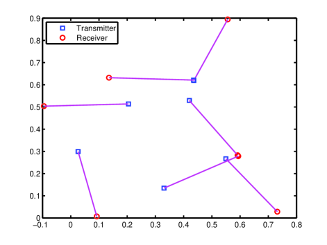
Figure 1: An example wireless network with 7 links, where square nodes are transmitters, and round nodes are receivers.

Fig. 2 shows the convergence results of the cost function (the bottom sub-figure) with slowly converging sources (the top sub-figure) after a simulation of $10^{5}$ time slots. In the simulation, we choose $\epsilon=10^{-3}$ and $\beta=5\times 10^{3}$. It can be observed from the top sub-figure that our algorithm achieves the optimal cost. Further, by comparing the convergence results of the cost and the arrival processes, we can conclude that Algorithm 1 can track the uncertain parameter $\boldsymbol{a}$ dynamically. In the simulation, it is further observed that the maximum queue length in the network is around $10^{2}$, so that the constraint in (68) is clearly satisfied.

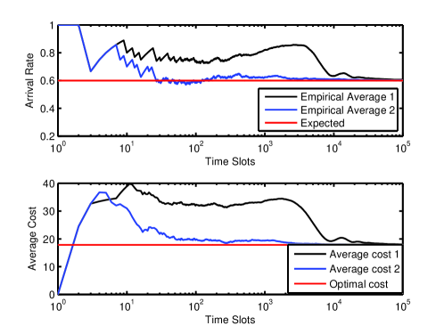
Figure 2: Convergence results of average cost with sources with different convergence behaviors.

VI Conclusion

In this paper we formulated a general class of scheduling problems in wireless networks with uncertain parameters, subject to the constraint that these parameters can be obtained from the empirical average values of certain stochastic network processes. We proposed a class of primal-dual type scheduling algorithms, and showed its optimality as well as feasibility using fluid limits.

[Proof of Lemma 6]

Proof:

We first prove 1). Let a sequence of functions $({\boldsymbol{T}}^{r_{n}},{\boldsymbol{Y}}^{r_{n}},{\boldsymbol{Z}}^{r_{n}})$ be given, which converge to a fluid limit $(\bar{\boldsymbol{T}},\bar{\boldsymbol{Y}},\bar{\boldsymbol{Z}})$. In the fluid limit, suppose that there is time $t>0$, $m\in\mathcal{M}$ and resource allocation modes $j,k$ such that

$$(\nabla_{m}\bar{g}(t))_{j}\geq(\nabla_{m}\bar{g}(t))_{k}+\epsilon$$ (69)

where $\epsilon>0$ is a small constant. Then, since $\nabla_{m}\bar{g}(t)$ is a continuous function of variable $t$, there is $\delta_{1}>0$ such that for all $\tau\in(t-\delta_{1},t+\delta_{1})$, we have

$$(\nabla_{m}\bar{g}(\tau))_{j}\geq(\nabla_{m}\bar{g}(\tau))_{k}+\epsilon/2$$ (70)

Further, since $\nabla_{m}\bar{g}(\tau)\triangleq\nabla_{m}g(\bar{\boldsymbol{x}}(\tau),\bar{\boldsymbol{z}}(\tau);\bar{\boldsymbol{y}}(\tau)))$ is continuous as a function of variables $(\bar{\boldsymbol{x}}(\tau),\bar{\boldsymbol{y}}(\tau),\bar{\boldsymbol{z}}(\tau))$ (and therefore is absolutely continuous when restricted to a compact local region), there is an $\epsilon^{\prime}>0$ such that $\|(\boldsymbol{x},\boldsymbol{y},\boldsymbol{z})-(\bar{\boldsymbol{x}}(\tau),\bar{\boldsymbol{y}}(\tau),\bar{\boldsymbol{z}}(\tau))\|\leq\epsilon^{\prime}$ implies that

$$\big{(}\nabla_{m}g\big{(}{\boldsymbol{x}},{\boldsymbol{z}};{\boldsymbol{y}})\big{)}_{j}\geq\big{(}\nabla_{m}g(\bar{\boldsymbol{x}}(\tau),\bar{\boldsymbol{z}}(\tau);\bar{\boldsymbol{y}}(\tau))\big{)}_{k}+\epsilon/4$$

for all $\tau\in(t-\delta_{1},t+\delta_{1})$. Now we define

$$({\boldsymbol{x}}^{r_{n}})^{(m)}(\tau) \triangleq \boldsymbol{T}^{(m)}(r_{n}\tau)/\boldsymbol{1}^{T}\boldsymbol{T}^{(m)}(r_{n}\tau)$$ (71)

$${\boldsymbol{y}}^{r_{n}}(\tau) \triangleq \boldsymbol{Y}(r_{n}\tau)/r_{n}\tau$$ (72)

$${\boldsymbol{z}}^{r_{n}}(\tau) \triangleq \boldsymbol{Z}(r_{n}\tau)/r_{n}\tau$$ (73)

Then, the definition of fluid limits implies that there exists $N\in\mathbb{N}$ and $\delta_{2}>0$ such that for all $n>N$ and $\tau\in(t-\delta_{2},t+\delta_{2})$,

$$\|({{\boldsymbol{x}}^{r_{n}}(\tau)},{{\boldsymbol{y}}}^{r_{n}}(\tau),{{\boldsymbol{z}}}^{r_{n}}(\tau))-(\bar{\boldsymbol{x}}(\tau),\bar{\boldsymbol{y}}(\tau),\bar{\boldsymbol{z}}(\tau))\|<\epsilon^{\prime}$$ (74)

Thus, by taking $\delta=\min(\delta_{1},\delta_{2})$ we have

$$\big{(}\nabla_{m}g\big{(}{{\boldsymbol{x}}^{r_{n}}(\tau)},{{\boldsymbol{z}}}^{r_{n}}(\tau);{{\boldsymbol{y}}}^{r_{n}}(\tau)\big{)}_{j}$$

$$\geq\big{(}\nabla_{m}g({{\boldsymbol{x}}^{r_{n}}(\tau)},{{\boldsymbol{z}}}^{r_{n}}(\tau);{{\boldsymbol{y}}}^{r_{n}}(\tau)\big{)}_{k}+\epsilon/4$$

for all $\tau\in(t-\delta,t+\delta)$. Further, by comparing the above definitions of ${{\boldsymbol{x}}^{r_{n}}(\tau)},{{\boldsymbol{y}}}^{r_{n}}(\tau)$ and ${{\boldsymbol{z}}}^{r_{n}}(\tau)$ to that of $\boldsymbol{x}(\tau)$, $\boldsymbol{y}(\tau)$ and $\boldsymbol{z}(\tau)$ in (19), (21) and (22), respectively, we conclude that they are essentially the same, except a difference in time scale, i.e., $\boldsymbol{x}^{r_{n}}(t)=\boldsymbol{x}(r_{n}t)$. Thus, the following holds in the original system: for any $n>N$ and all $\tau\in(r_{n}(t-\delta),r_{n}(t+\delta))$,

$$\big{(}\nabla_{m}g({{\boldsymbol{x}}(\tau)},{{\boldsymbol{z}}}(\tau);{{\boldsymbol{y}}}(\tau)\big{)}_{j}\geq\big{(}\nabla_{m}g({{\boldsymbol{x}}(\tau)},{{\boldsymbol{z}}}(\tau);{{\boldsymbol{y}}}(\tau)\big{)}_{k}+\epsilon/4$$

Therefore, according to Lemma 3, $\xi^{(m)}_{j}$ is never chosen in any time slot during $(r_{n}(t-\delta),r_{n}(t+\delta))$, and we have that $T_{j}^{(m)}(\tau)$ is a constant during $(r_{n}(t-\delta),r_{n}(t+\delta))$, from which we conclude that $\dot{\bar{T}}_{j}^{(m)}(t)=0$. Therefore, $\bar{v}^{(m)}_{j}(t)=0$ following the definition that $\bar{v}_{j}^{(m)}(t)=\dot{\bar{T}}_{j}^{(m)}(t)/\pi^{(m)}$.

We next prove 2). Let $\bar{\boldsymbol{u}}$ be given as a feasible point of GRAD-ZBAR and $\epsilon>0$ be given. Since $\nabla_{\boldsymbol{z}}g(\cdot)$ is a continuous function of $t$, there is $\delta>0$ and $N\in\mathbb{N}$ such that for $n>N$ and all $\tau<(t-\delta,t+\delta)$, the following holds:

$$\|\nabla_{\boldsymbol{z}}g({{\boldsymbol{x}}^{r_{n}}(\tau)},{{\boldsymbol{z}}}^{r_{n}}(\tau);{{\boldsymbol{y}}}^{r_{n}}(\tau))-\nabla_{\boldsymbol{z}}{g}(\bar{\boldsymbol{x}}(t),\bar{\boldsymbol{z}}(t);\bar{\boldsymbol{y}}(t))\|<\epsilon$$ (75)

Further, note that Lemma 3 implies that for any time slot in $(r_{n}(t-\delta),r_{n}(t+\delta))$, we have

$$\nabla_{\boldsymbol{z}}g({{\boldsymbol{x}}(\tau)},{{\boldsymbol{z}}(\tau)};\boldsymbol{y}(\tau))^{T}\boldsymbol{u}(\tau)\leq\nabla_{\boldsymbol{z}}g({\boldsymbol{x}}(\tau),{\boldsymbol{z}}(\tau);\boldsymbol{y}(\tau))^{T}\bar{\boldsymbol{u}}$$

Thus, applying (75) to the above inequality we have

$$\nabla_{\boldsymbol{z}}{g}(\bar{\boldsymbol{x}}(t),\bar{\boldsymbol{z}}(t);\bar{\boldsymbol{y}}(t))^{T}\boldsymbol{u}(\tau)\leq\nabla_{\boldsymbol{z}}{g}(\bar{\boldsymbol{x}}(t),\bar{\boldsymbol{z}}(t);\bar{\boldsymbol{y}}(t))^{T}\bar{\boldsymbol{u}}+c\epsilon$$

for all $\tau\in(r_{n}(t-\delta),r_{n}(t+\delta))$, where $c>0$ is a proper constant. After summing over $(r_{n}(t-\delta),r_{n}(t+\delta))$ and dividing by $r_{n}$ on both sides, we obtain

$$\nabla_{\boldsymbol{z}}{g}(\bar{\boldsymbol{x}}(t),\bar{\boldsymbol{z}}(t);\bar{\boldsymbol{y}}(t))^{T}(\boldsymbol{Z}^{r_{n}}(t+\delta)-\boldsymbol{Z}^{r_{n}}(t-\delta))$$

$$\leq 2\delta(\nabla_{\boldsymbol{z}}{g}(\bar{\boldsymbol{x}}(t),\bar{\boldsymbol{z}}(t);\bar{\boldsymbol{y}}(t))^{T}\bar{\boldsymbol{u}}+c\epsilon)$$

Finally, we let $n\rightarrow\infty$, and noting that $\delta>0$ can be taken arbitrarily small, we have

$$\nabla_{\boldsymbol{z}}{g}(\bar{\boldsymbol{x}}(t),\bar{\boldsymbol{z}}(t);\bar{\boldsymbol{y}}(t))^{T}\bar{\boldsymbol{u}}(t)\leq\nabla_{\boldsymbol{z}}{g}(\bar{\boldsymbol{x}}(t),\bar{\boldsymbol{z}}(t);\bar{\boldsymbol{y}}(t))^{T}\bar{\boldsymbol{u}}+c\epsilon$$

from which 2) holds since $\epsilon>0$ is arbitrary. ∎

References

• [1] L. Tassiulas and A. Ephremides, “Stability properties of constrained queuing systems and scheduling policies for maximum throughput in multihop radio networks,” IEEE Trans. on Automatic Control, Vol. 37, No. 12, pp. 1936-1949, December 1992
• [2] M. J. Neely, “Energy Optimal Control for Time Varying Wireless Networks”, IEEE Transactions on Information Theory, vol. 52, no. 7, pp. 2915-2934, July 2006
• [3] B. Hajek and G. Sasaki, “Link scheduling in polynomial time,” IEEE Trans. Information Theory, Vol. 34, Sept. 1988, pp. 910 - 917
• [4] L. Georgiadis, M. J. Neely, L. Tassiulas, “Resource Allocation and Cross-Layer Control in Wireless Networks,”, Foundations and Trends in Networking, Vol. 1, no. 1, pp. 1-144, 2006.
• [5] M. J. Neely, “Stochastic Network Optimization with Non-Convex Utilities and Costs,” Proc. Information Theory and Applications Workshop (ITA), Feb. 2010.
• [6] A.L. Stolyar, “Maximizing Queuing Network Utility subject to Stability: Greedy Primal-Dual Algorithm,”Queuing Systems, 2005, Vol. 50, No.4, pp.401-457
• [7] A. Eryilmaz and R. Srikant. “Joint Congestion Control, Routing and MAC for Stability and Fairness in Wireless Networks,” IEEE Journal on Selected Areas in Communications, August 2006, 1514-1524.
• [8] A. Eryilmaz, and R. Srikant, “Fair Resource Allocation in Wireless Networks using Queue-length based Scheduling and Congestion Control”, IEEE/ACM Trans. on Networking, Jan., 2007, pp. 1333-1344.
• [9] F. P. Kelly, A.K. Maulloo and D.K.H. Tan, “Rate control in communication networks: shadow prices, proportional fairness and stability, ”, Journal of the Operational Research Society, Vol. 49 (1998), 237-252
• [10] S. Shakkottai and R. Srikant, “Network Optimization and Control,” Foundations and Trends in Networking, NoW Publishers, 2007.
• [11] D. P. Bertsekas, “Nonlinear Programming”, Athena Scientific, 2nd Edition, 1999.
• [12] J.G. Dai and B. Prabhakar, “The throughput of data switches with and without speedup,” Proc. of the IEEE INFOCOM, 2:556-564, March 2000
• [13] H. Royden, “Real Analysis”, Prentice Hall, 3rd Edition, 1988.