Functional integral for non-Lagrangian systems

Abstract

A novel functional integral formulation of quantum mechanics for non-Lagrangian systems is presented. The new approach, which we call “stringy quantization,” is based solely on classical equations of motion and is free of any ambiguity arising from Lagrangian and/or Hamiltonian formulation of the theory. The functionality of the proposed method is demonstrated on several examples. Special attention is paid to the stringy quantization of systems with a general $A$-power friction force $-\kappa\dot{q}^{A}$. Results for $A=1$ are compared with those obtained in the approaches by Caldirola-Kanai, Bateman and Kostin. Relations to the Caldeira-Leggett model and to the Feynman-Vernon approach are discussed as well.

Dedicated to my father on the occasion of his 60th birthdays.

I Introduction

Quantization is a phenomenon that changes our bright classical perspective into a bit uncertain and at first sight rather nonintuitive picture. This picture, however, is more rigorous than the classical one, possesses many fascinating features and has produced a lot of successful predictions.

The subtle problem of transition from classical to quantal attracts attention from the early days of quantum mechanics. Over the years various techniques and methods for solving this puzzle have been invented. Our aim is not to trace back the complete (hi)story of the milestone ideas in this field (for the review we refer to englis ). What we want to do is to give a concise exposition of the method we have developed. However, since we have generalized the original Feynman’s path integral approach, we will recapitulate this approach shortly in section II.

The main goal of our paper is to obtain a functional integral formula for the quantum propagator which would not refer to Lagrangian and/or Hamiltonian function. Quantum propagator is the probability amplitude $\mathbf{A}(q_{1},t_{1}\,|\,q_{0},t_{0})$ for the transition of the system from the initial configuration $(q_{0},t_{0})$ to the final configuration $(q_{1},t_{1})$. We will derive a closed expression for this quantity starting from the given set of classical dynamical equations of motion.

The proposed method uses functional integration in the extended phase space, but instead of integration over path histories we introduce integration over stringy surfaces. This crucial element of our approach is explained in full detail in sections III and IV and in appendices A and B. We also make sure that whenever the system under consideration becomes Lagrangian, the stringy description reduces to the standard one with the Feynman path integral.

In sections V and VI some simple examples are scrutinized. It is well known that there are classical dynamical systems that cannot be described within the traditional Lagrangian or Hamiltonian framework. The stringy approach enables us to quantize them straightforwardly. In section V the quantization of a weakly non-Lagrangian system is performed. The transition amplitude is computed for a particle in a conservative field, whose motion is damped by a general $A$-power friction force $F=-\kappa\dot{q}^{A}$. The stringy results for $A=1$ are compared with the results obtained in the approaches by Caldirola-Kanai CK , Bateman bateman and Kostin kostin .

One can argue against the stringy quantization of dissipative systems that it is unable to describe decoherence phenomena. This is true, but the same objection can be raised against the generally accepted heuristic approaches by the authors cited above, as well as those by Dekker dekker2 , Razavy razavy2 , Geicke geicke and others, simply because their kinematical and dynamical prerequisites are different from the prerequisites of the particle-plus-environment quantum models. However, a possible argument for the stringy quantization is that the particle-plus-environment models are not able to handle satisfactorily the case with the friction force $-\kappa\dot{q}^{A}$ for the general power $A$. Moreover, they describe a rather different phenomenon, namely the quantum Brownian motion for which the total force equals $-\kappa\dot{q}+\mbox{\emph{stochastic term}}$.

Section VI contains the analysis of a curious two-dimensional Douglas system douglas which is strongly non-Lagrangian, i.e. not derivable from any sort of Lagrangian or Hamiltonian. This causes a fundamental problem for all conventional quantization methods, but can be dealt with in a rather transparent way in the stringy approach.

In section VII conclusion, discussion and outlook are collected. The section also includes some comments on the relation between the stringy quantization and the Caldeira-Leggett model of quantum Brownian motion particle+environment , as well as the influence functional technique by Feynman and Vernon feynman-vernon .

Some rather technical material is left to appendices. Appendix A is devoted to the stringy variational principle, which plays an important role in the motivation of our approach. In appendix B computational details concerning the surface functional integral for quantum friction force systems are presented.

Historically the first attempt at quantization based on the dynamical equations of motion belongs to Feynman, see dyson . A similar problem was considered by Wigner, Yang $\&$ Feldman, Nelson, Okubo and others, see w-yf-o . Among the recent investigations in this field let us mention the work of Lyakhovich $\&$ Sharapov sharapov and Gitman $\&$ Kupriyanov gitman . They consider the same problem as us, but their strategy is different. In our opinion, their approach fits much better the context of gauge field dynamics.

As Ludwig Faddeev noted during the Edward Witten’s talk at the Mathematical Physics Conference: From XX To XXI Century, quantization is not a science, quantization is an art. Let us believe that the quantization method proposed here will fit the Ludwig’s dictum and will be meaningful enough to be considered artistic.

II Feynman Quantum Mechanics

According to Feynman feynman , the probability amplitude of the transition of the system from the space-time configuration $(q_{0},t_{0})$ to another space-time configuration $(q_{1},t_{1})$ is

$$\mathbf{A}(q_{1},t_{1}\,|\,q_{0},t_{0})=\frac{1}{\mathbf{N}}\int[\mathscr{D}\tilde{\gamma}]\exp{\Bigl{\{}\frac{i}{\hslash}\int\limits_{\tilde{\gamma}}pdq-Hdt\Bigr{\}}}\,.$$ (1)

Here the integral is taken over all paths (histories) $\tilde{\gamma}(t)=(\tilde{q}(t),\tilde{p}(t),t)$ in the extended phase space , satisfying the conditions $\tilde{q}(t_{0})=q_{0}$ and $\tilde{q}(t_{1})=q_{1}$.

The preexponential factor $1/\mathbf{N}$ in the expression (1) serves just the normalization. To fix it properly we impose two physical conditions on the transition amplitude. First we introduce an integral condition that ensures that the total probability is conserved,

$$\int dq_{1}\,\overline{\bm{\mathbf{A}}}(q_{1},t_{1}\,|\,q_{0},t_{0})\,\mathbf{A}(q_{1},t_{1}\,|\,q^{\prime}_{0},t_{0})=\delta(q_{0}-q^{\prime}_{0})\,.$$ (2a)

This specifies the absolute value of $$\mathbf{N} t_{1} t_{0}$$. Then we add a constraint that expresses the obvious fact that no evolution takes place if the final time approaches the initial time ,

$$\lim\limits_{t_{1}\rightarrow t_{0}}\mathbf{A}(q_{1},t_{1}\,|\,q_{0},t_{0})=\delta(q_{1}-q_{0})\,.$$ (2b)

This determines the phase of $\mathbf{N}$.

A miraculous consequence of the definition of the transition amplitude (1) (not an additional requirement!) is that it satisfies the evolutionary chain rule, or Chapman-Kolmogorov equation,

$$\mathbf{A}(q_{1},t_{1}\,|\,q_{0},t_{0})=\int dq^{\prime}\mathbf{A}(q_{1},t_{1}\,|\,q^{\prime},t)\,\mathbf{A}(q^{\prime},t\,|\,q_{0},t_{0})\,.$$ (3)

The infinitesimal version of this formula is the celebrated Schrödinger equation.

Quantum states of the system are described by the square integrable functions with the standard Hilbert space structure. Physical observables are hermitian operators acting on such functions. Given the state $\Psi_{0}(q)$ at the initial moment $t_{0}$ one is able to predict the state $\Psi_{1}(q)$ at any later moment $t_{1}$ according to the formula

$$\Psi_{0}(q)\ \rightsquigarrow\ \Psi_{1}(q)=\int dq^{\prime}\,\mathbf{A}(q,t_{1}\,|\,q^{\prime},t_{0})\Psi_{0}(q^{\prime})\,.$$ (4)

In what follows it is assumed that the above concept of states, observables and quantum evolution is valid for the stringy quantization of non-Lagrangian systems as well. The only new element is a modified prescription for the evolutionary integral kernel $\mathbf{A}(q_{1},t_{1}\,|\,q_{0},t_{0})$. The same kinematical prerequisites can be found also in other phenomenological approaches CK -geicke .

III One step beyond Feynman

A possible step beyond the theory summarized above consists in the elimination of the Hamiltonian function $H$ from formula (1). The price to be paid is the replacement of the path integration by the surface functional integration.

Our aim is to construct the amplitude for the transition between $(q_{0},t_{0})$ and $(q_{1},t_{1})$ starting from the classical equations of motion (and not from the Hamiltonian function which provides them)

$$\dot{q}^{a}=\frac{\partial H}{\partial p_{a}}\equiv\frac{p^{a}}{m}\,,\quad\dot{p}_{a}=-\frac{\partial H}{\partial q^{a}}\equiv F_{a}\,.$$ (5)

In the first set of equations, $m$ is the mass of the particle. We restricted ourselves to the simplest case of one particle, although it is trivial to generalize the theory to a system with an arbitrary number of particles. Note also that if the particle is unconstrained and we make use of Cartesian coordinates, the momenta $p^{a}$ defined in (5) reduce to $p_{a}$.

Suppose that there exists a unique classical trajectory in the extended phase space $\gamma_{cl}(t)=(q_{cl}(t),p_{cl}(t),t)$, connecting the points $(q_{0},t_{0})$ and $(q_{1},t_{1})$. Then we can assign to any other trajectory $\tilde{\gamma}(t)=(\tilde{q}(t),\tilde{p}(t),t)$, which enters the path integral in (1), two auxiliary curves

$$\lambda_{0}(s) = \bigl{(}q_{0},\pi(s),t_{0}\bigr{)},\ \mbox{where}\ \pi(0)=p_{cl}(t_{0}),\ \pi(1)=\tilde{p}(t_{0});$$

$$\lambda_{1}(s) = \bigl{(}q_{1},\phi(s),t_{1}\bigr{)},\ \mbox{where}\ \phi(0)=p_{cl}(t_{1}),\ \phi(1)=\tilde{p}(t_{1}).$$

The curves are parameterized by the parameter $s\in[0,1]$ and live in the momentum subsectors of the extended phase space with fixed $(q_{0},t_{0})$ and $(q_{1},t_{1})$, see Figure 1.

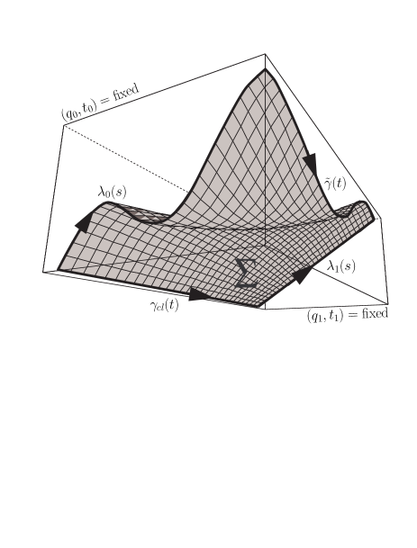
Figure 1: Schematic picture of two auxiliary curves $\lambda_{0}(s)$ and $\lambda_{1}(s)$ which connect the classical history $\gamma_{cl}(t)$ with the given history $\tilde{\gamma}(t)$ in the extended phase space. $\lambda$-curves are located in the $n$-dimensional subspaces of the extended phase space in which the momenta are varying while the coordinates and time are kept fixed. The contour $\partial\Sigma=\tilde{\gamma}-\lambda_{1}-\gamma_{cl}+\lambda_{0}$ forms a boundary for plenty of extended phase space surfaces. One of them, denoted as $\Sigma$, is drawn in the figure.

Using these definitions one can write

$$\int\limits_{\tilde{\gamma}}p_{a}dq^{a}-Hdt=\int\limits_{\gamma_{cl}}p_{a}dq^{a}-Hdt+\oint\limits_{\partial\Sigma}p_{a}dq^{a}-Hdt\,,$$ (6)

where $\partial\Sigma=\tilde{\gamma}-\lambda_{1}-\gamma_{cl}+\lambda_{0}$ is a contour in the extended phase space consisting of four curves $\tilde{\gamma}(t)$, $\gamma_{cl}(t)$, $\lambda_{0}(s)$, $\lambda_{1}(s)$. The first integral on the right hand side is the classical action $\mathbf{S}_{cl}(q_{1},t_{1}\,|\,q_{0},t_{0})$ (its equivalent for the non-Lagrangian case will be specified later), while the second integral can be rewritten as

$$\oint\limits_{\partial\Sigma}p_{a}dq^{a}-Hdt=\int\limits_{\Sigma}dp_{a}\wedge\Bigl{(}dq^{a}-\frac{\partial H}{\partial p_{a}}dt\Bigr{)}-\frac{\partial H}{\partial q^{a}}dq^{a}\wedge dt\,,$$

where $\Sigma$ is a surface spanning the contour $\partial\Sigma$, i. e. a map from the parametric space $(t,s)\in[t_{0},t_{1}]\times[0,1]$ to the extended phase space,

$$\Sigma:(t,s)\mapsto\Sigma(t,s)\equiv\bigl{(}q^{a}(t,s),p_{a}(t,s),t(t,s)=t\bigr{)}\,,$$

satisfying

$${\Sigma(t,0)=\gamma_{cl}(t)\atop\Sigma(t,1)=\tilde{\gamma}(t)\ \,}\ \ \ \ \mbox{and}\ \ \ \ {\Sigma(t_{0},s)=\lambda_{0}(s)\atop\Sigma(t_{1},s)=\lambda_{1}(s)}\,.$$

The surface $\Sigma$ can be viewed as a worldsheet of a string, therefore we will call the quantization method using such surfaces “stringy.” Partial derivatives of the Hamiltonian function entering the integral over $\Sigma$ can be eliminated with the help of the equations of motion (5). By doing so, one transforms (6) into the following form:

$$\int\limits_{\tilde{\gamma}}p_{a}dq^{a}-Hdt=\mathbf{S}_{cl}(q_{1},t_{1}\,|\,q_{0},t_{0})+\int\limits_{\Sigma}\Omega\,,$$ (7)

where the two-form $\Omega$ is defined as

$$\Omega=dp_{a}\wedge dq^{a}-\Bigl{(}\frac{p^{a}}{m}dp_{a}-F_{a}dq^{a}\Bigr{)}\wedge dt\,.$$ (8)

This two-form is an object in the extended phase space and its structure can be read out from the underlying equations of motion. Note that for non-potential forces the expression $(p^{a}/m)dp_{a}-F_{a}dq^{a}$ does not reduce to $dH$, so that the two-form $\Omega$ is not closed. This becomes essential in the next subsection.

It is obvious that for a given pair of histories $(\tilde{\gamma},\gamma_{cl})$ there exist infinitely many $\Sigma$-surfaces such that $\tilde{\gamma}-\gamma_{cl}\subset\partial\Sigma$. All of them form a set which we will call $\mathscr{U}_{(\tilde{\gamma},\gamma_{cl})}$ . Since no $\Sigma$ is preferred and $\int_{\Sigma}\Omega$ is only boundary dependent, it is natural to average the exponent of (7) over the whole stringy set $\mathscr{U}_{(\tilde{\gamma},\gamma_{cl})}$. After doing so we obtain the identity

$$\exp{\Bigl{\{}\frac{i}{\hslash}\int\limits_{\tilde{\gamma}}p_{a}dq^{a}-Hdt\Bigr{\}}}=\frac{\mbox{\large{e}}^{\frac{i}{\hslash}\mathbf{S}_{cl}}}{\mathrm{N}_{\tilde{\gamma}}}\int\limits_{\mathscr{U}_{(\tilde{\gamma},\gamma_{cl})}}[\mathscr{D}\Sigma]\exp{\Bigl{\{}\frac{i}{\hslash}\int\limits_{\Sigma}\Omega\Bigr{\}}},$$

where $\mathrm{N}_{\tilde{\gamma}}$ is the cardinality of the stringy set $\mathscr{U}_{(\tilde{\gamma},\gamma_{cl})}$, $\mathrm{N}_{\tilde{\gamma}}:=\#\mathscr{U}_{(\tilde{\gamma},\gamma_{cl})}$, and $[\mathscr{D}\Sigma]$ is a functional integration measure specified in Appendix B. If no topology-related problems arise in the extended phase space, the infinite constant $\mathrm{N}_{\tilde{\gamma}}$ is independent of the history $\tilde{\gamma}$. Taking all this into account we can rewrite (1) as

$${}\boxed{\vspace{5mm}\hskip 2.84526pt\mathbf{A}(q_{1},t_{1}\,|\,q_{0},t_{0})\,=\,\frac{\mbox{\large{e}}^{\frac{i}{\hslash}\mathbf{S}_{cl}}}{\mathbf{N}}\int\limits_{\mathscr{U}_{\gamma_{cl}}}[\mathscr{D}\Sigma]\exp{\Bigl{\{}\frac{i}{\hslash}\int\limits_{\Sigma}\Omega\Bigr{\}}},\hskip 5.69054pt}$$ (9)

where the set $\mathscr{U}_{\gamma_{cl}}$ over which the functional integration is carried out contains all strings in the extended phase space which are anchored to the given classical trajectory $\gamma_{cl}$. Some surfaces from $\mathscr{U}_{\gamma_{cl}}$ are depicted in Figure 2. In (9), the undetermined constant $1/\mathrm{N}_{\tilde{\gamma}}$ was absorbed into the overall preexponential factor $1/\mathbf{N}$ and the path integral over $\tilde{\gamma}$’s was converted into the surface functional integral, as promised earlier, using the identities

$$\int[\mathscr{D}\tilde{\gamma}]\int\limits_{\ \ \ \mathscr{U}_{(\tilde{\gamma},\gamma_{cl})}}[\mathscr{D}\Sigma]\cdots\ =\int\limits_{\ \ \ \bigcup_{\tilde{\gamma}}\mathscr{U}_{(\tilde{\gamma},\gamma_{cl})}}[\mathscr{D}\Sigma]\cdots\ =\int\limits_{\mathscr{U}_{\gamma_{cl}}}[\mathscr{D}\Sigma]\cdots\ \,.$$ (10)

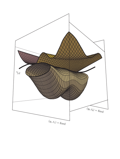
Figure 2: Four elements (two open, one closed and one shrunk to $\gamma_{cl}$) of $\mathscr{U}_{\gamma_{cl}}$, anchored to the given classical history $\gamma_{cl}$ in the extended phase space. The two open surfaces belong to two different stringy classes $\mathscr{U}_{(\tilde{\gamma},\gamma_{cl})}$, while the closed and the shrunk surface are both elements of the same stringy class $\mathscr{U}_{(\gamma_{cl},\gamma_{cl})}$. As the worldsheet $\Sigma$ varies, the front and rear boundary curves, denoted in the text $\lambda_{0}$ and $\lambda_{1}$, vary as well.

IV One more step beyond – non-Lagrangian systems

In case the Hamiltonian function $H$ is given, the formula (9) for the propagator is equivalent to the Feynman formula (1) we have started with. The surface functional integral (9) is however completely free of $H$ and requires just the knowledge of the classical equations of motion. This observation allows us to postulate (9) as a quantization tool in situations in which one cannot use the standard Hamiltonian approach. We just have to relax the requirement of the closedness of the two-form $\Omega$, following from the definition of $\Omega$ for Hamiltonian systems. This relaxation is what is hidden behind the slightly provocative phrase one more step beyond in the title of this subsection.

The problematic part here is the definition of the classical action $\mathbf{S}_{cl}(q_{1},t_{1}\,|\,q_{0},t_{0})$ for non-Lagrangian systems. Later we will see that in some specific situations this quantity can be read out from the structure of the surface integral

$$\int\limits_{\mathscr{U}_{\gamma_{cl}}}[\mathscr{D}\Sigma]\exp{\Bigl{\{}\frac{i}{\hslash}\int\limits_{\Sigma}\Omega\Bigr{\}}}\,.$$

Another possibility which comes to mind is to use the integrating factor of the generally non-closed two-form $\Omega$. This means that one will look for a function $f(q,p,t)$ on the extended phase space such that $d(f\Omega)=0$. If the structure of the dynamical equations allows for such a function (i.e. the forces satisfy the Helmholtz condition) then we can define a local auxiliary Hamiltonian $H_{aux}$ such that $f\Omega=d(p_{a}dq^{a}-H_{aux}dt)$. Having $H_{aux}$ we can define the auxiliary classical action $\mathbf{S}_{aux}$. The alternative approach which tries to identify $\mathbf{S}_{cl}$ with $\mathbf{S}_{aux}$ has, however, several substantial disadvantages. First of all, the procedure of finding $f$ (and subsequently $H_{aux}$ and $\mathbf{S}_{aux}$) is highly ambiguous. Furthermore, $\mathbf{S}_{aux}$ lacks symmetries that were originally present in the equations of motion. Because of these findings we do not follow this strategy hereinafter.

From the physical point of view the dynamical equations seem to be more fundamental than their compact but ambiguous precursors, Hamiltonian and/or Lagrangian function, see guys . Since (9) requires just the knowledge of the equations of motion, it determines the transition amplitude in a completely new way.

Our proposal for the transition amplitude has appeared here out of thin air. Actually, we were rewriting (1) in terms of stringy surfaces and then, when realizing that the integrated function can be written without any reference to the Hamiltonian, we postulated formula (9) to be valid in general. However, this is not the whole story. The stringy functional quantization can be motivated also by the stringy variational principle. Having the dynamical equations and initial and final endpoints, one can form $\mathscr{U}_{\gamma_{cl}}$ and $\Omega$. Then using these objects one can introduce the stringy action functional

$$\mathscr{S}:\mathscr{U}_{\gamma_{cl}}\rightarrow\mathbb{R}\,,\ \ \ \ \ \Sigma\mapsto\mathscr{S}(\Sigma):=\int\limits_{\Sigma}\Omega\,.$$ (11)

This is a variational problem with varying boundaries, therefore the total variation has two terms. First one specifies the boundary and determines the initial equations of motion for $\gamma_{cl}$. The second one specifies the bulk of the stationary world-sheet $\Sigma$ (which turns out to be shrunk into $\gamma_{cl}$ itself). Moreover, one immediately verifies that in the special case when $\Omega=d(p_{a}dq^{a}-Hdt)$, the stringy variational principle reduces (up to an additive constant) to the celebrated Hamilton least action principle. Of course, many subtleties were omitted here, but all of them can be found in kochan , or in Appendix A. Thus, our variational principle enables us to perform the limit $\hslash\rightarrow 0$, in which we recover the original classical dynamics as required.

V Quantization of friction force systems

To examine the functionality of the proposed quantization method let us first analyze the simplest friction force system. It consists of a particle with unit mass, moving in one dimension under the action of the conservative force $F=-dU/dq$ and the friction force $-\kappa\dot{q}^{A}$ . Thus,

$$\ddot{q}=-\kappa\dot{q}^{A}+F\,\Rightarrow\,\Omega=d\bigl{(}pdq-\tfrac{1}{2}p^{2}dt-Udt\bigr{)}-\kappa p^{A}\,dq\wedge dt\,.$$

In this example the surface functional integral can be calculated explicitly (for more detail see kochan , or Appendix B). In the course of calculation, the surface functional integral in the extended phase space reduces to path integral in the configuration space,

$$\int\limits_{\mathscr{U}_{\gamma_{cl}}}[\mathscr{D}\Sigma]\exp{\Bigl{\{}\frac{i}{\hslash}\int\limits_{\Sigma}\Omega\Bigr{\}}}\propto$$ (12)

$$\propto\exp{\Bigl{\{}-\frac{i}{\hslash}\int\limits_{t_{0}}^{t_{1}}\bigl{(}\tfrac{1}{2}\dot{q}_{cl}^{2}-U(q_{cl})-\kappa q_{cl}p^{A}_{cl}\bigr{)}dt\Bigr{\}}}\times$$

$$\times\int[\mathscr{D}q]\exp{\Bigl{\{}\frac{i}{\hslash}\int\limits_{t_{0}}^{t_{1}}\bigl{(}\tfrac{1}{2}\dot{q}^{2}-U(q)-\kappa qp^{A}_{cl}\bigr{)}dt\Bigr{\}}}\,.$$

This combined with the formula (9) suggests that it will be convenient to define the classical action as

$$\mathbf{S}_{Acl}(q_{1},t_{1}|q_{0},t_{0})=\int\limits_{t_{0}}^{t_{1}}\bigl{(}\tfrac{1}{2}\dot{q}_{cl}^{2}-U(q_{cl})-\kappa q_{cl}p^{A}_{cl}\bigr{)}dt\,.$$ (13)

When doing so, we obtain a controlled cancelation of $\exp\{\frac{i}{\hslash}\mathbf{S}_{Acl}\}$ with the preexponential factor arising from (12). The final probability amplitude then assumes a compact and reasonable form:

$$\mathbf{A}_{Astr}(q_{1},t_{1}|q_{0},t_{0})=$$

$$=\frac{1}{\mathbf{N}_{Astr}}\int[\mathscr{D}q]\exp{\Bigl{\{}\frac{i}{\hslash}\int\limits_{t_{0}}^{t_{1}}\bigl{(}\tfrac{1}{2}\dot{q}^{2}-U(q)-\kappa qp^{A}_{cl}\bigr{)}dt\Bigr{\}}}\,.$$ (14)

The preexponential factor $1/\mathbf{N}_{Astr}$ can in principle be obtained by subjecting $\mathbf{A}_{Astr}(q_{1},t_{1}|q_{0},t_{0})$ to the conditions (2).

Let us explain why one should consider the propagator formula (V) reasonable. In the path integral above there appears an unconventional “external source” term $-\kappa qp^{A}_{cl}$. Its appearance guarantees that the quantum dynamics governed by $\mathbf{A}_{Astr}(q_{1},t_{1}|q_{0},t_{0})$ transforms into classical mechanics in the limit $\hslash\to 0$. This follows from the simple fact that the unique solution of the saddle point equation for the path integral (V),

$$\ddot{q}=-\frac{dU}{dq}-\kappa\dot{q}^{A}_{cl}\,,$$

which satisfies the given initial and final conditions $q(t_{0})=q_{0}$ and $q(t_{1})=q_{1}$, is the classical trajectory $q_{cl}(t)$.

The external source term in (V) breaks the validity of the Chapman-Kolmogorov (memoryless) equation . From the physical point of view it is a desired phenomenon. The microscopic origin of friction is some environmental interaction. This, however, was not accounted for here explicitly. What has been considered is some effective (macroscopic, phenomenological) interaction emerging on the classical level only. Microscopically the system is a part of a larger system and hence it should be affected by the memory effect.

It is not difficult to compute $\mathbf{A}_{Astr}(q_{1},t_{1}|q_{0},t_{0})$ for the general power $A$ and the potentials $U(q)=0$ and $U(q)=\tfrac{1}{2}\omega^{2}q^{2}$. In both cases we can carry out the path integration in (V) explicitly to obtain

$$\mathbf{A}_{Astr}(q_{1},t_{1}|q_{0},t_{0})=$$

$$=\frac{1}{\mathbf{N}_{Astr}}\exp\left\{\frac{i}{\hslash}\mathbf{S}_{Acl}(q_{1},t_{1}|q_{0},t_{0})\right\}\,,$$ (15)

where the non-Lagrangian action $\mathbf{S}_{Acl}(q_{1},t_{1}|q_{0},t_{0})$ is given by the expression (13). An open problem is to determine the preexponential factor $1/\mathbf{N}_{Astr}(t_{1}-t_{0},q_{1},q_{0})$ for all powers $A$ except for $A=1$ (at least the author is incapable to do that). If $A\neq 1$, the preexponential factor is apparently dependent not only on the time difference $t_{1}-t_{0}$, but also on the endpoint positions $q_{0}$ and $q_{1}$. This hypothesis is supported by the results obtained in stuckens-kobe , where the path integral for a non-conservative force quadratic in velocity is calculated. The normalization prefactor which appears there is explicitly dependent on the endpoints positions as well as on $t_{1}-t_{0}$.

In what follows we will restrict ourself to the case when the power $A$ is equal to 1. This simplified setup enables us to compare the stringy approach with the Caldirola-Kanai, Bateman and Kostin approaches .

V.1 Stringy versus Caldirola-Kanai approach

The dissipative system under consideration is weakly non-Lagrangian. This means that $d\Omega\neq 0$, but $\Omega$ possesses a local integrator $f\neq 0$. Let us define the auxiliary Lagrangian function (one of plenty) as

$$L_{CK}(q,t) =e^{\kappa t}\Bigl{[}\tfrac{1}{2}\dot{q}^{2}-U(q)\Bigr{]}.$$ (16)

This Lagrangian is usually called CK-Lagrangian after its inventors P. Caldirola and E. Kanai CK . Henceforward a damped free particle is considered only, i.e. the potential energy $U(q)$ is supposed to be zero. It is immediately clear that the transition amplitude computed from (V) differs from the CK-amplitude

$$\mathbf{A}_{CK}(q_{1},t_{1}|q_{0},t_{0}) = \dfrac{1}{\mathbf{N}_{CK}}\int[\mathscr{D}q]\exp{\Bigl{\{}\frac{i}{\hslash}\int\limits_{t_{0}}^{t_{1}}L_{CK}(q,t)dt\Bigr{\}}}$$

$$= \dfrac{1}{\mathbf{N}_{CK}}\exp\{\tfrac{i}{\hslash}\,\mathbf{S}_{CK}(q_{1},t_{1}|q_{0},t_{0})\}\,.$$

Indeed, the stringy and CK actions which enter the corresponding transition amplitudes are different,

$$\mathbf{S}_{1cl}=\frac{\kappa}{4}(q_{1}-q_{0})\frac{(q_{0}+3q_{1})\mathrm{e}^{-\kappa t_{1}}-(q_{1}+3q_{0})\mathrm{e}^{-\kappa t_{0}}}{\mathrm{e}^{-\kappa t_{0}}-\mathrm{e}^{-\kappa t_{1}}},$$

$$\mathbf{S}_{CK}=\frac{\kappa}{2}\,\frac{(q_{1}-q_{0})^{2}}{\mathrm{e}^{-\kappa t_{0}}-\mathrm{e}^{-\kappa t_{1}}}.$$

Since both actions are quadratic functions of the endpoints $q_{0}$ and $q_{1}$, and since we require that the total probability is conserved, the preexponential factors for both transition amplitudes can be computed from the Van Vleck formula

$$\frac{1}{\mathbf{N}}=\sqrt{\frac{i}{2\pi\hslash}\,\frac{\partial^{2}\mathbf{S}}{\partial q_{1}\,\partial q_{0}}}\,.$$

Using this formula we arrive at the normalized transition amplitudes

$$\mathbf{A}_{1str}(q_{1},t_{1}|q_{0},t_{0}) = \sqrt{\frac{\kappa}{4\pi i\hslash\tanh\tfrac{\kappa}{2}(t_{1}-t_{0})}}\,\mbox{\large{e}}^{\frac{i}{\hslash}\mathbf{S}_{1cl}},$$ (17)

$$\mathbf{A}_{CK}(q_{1},t_{1}|q_{0},t_{0}) = \sqrt{\frac{\kappa}{2\pi i\hslash\,(\mathrm{e}^{-\kappa t_{0}}-\mathrm{e}^{-\kappa t_{1}})}}\,\mbox{\large{e}}^{\frac{i}{\hslash}\mathbf{S}_{CK}},$$ (18)

which trivially satisfy (2). Moreover, one immediately verifies that in the frictionless limit $\kappa\rightarrow 0$ both transition amplitudes coincide with the free particle propagator. A short inspection shows that the stringy propagator depends on $t_{0}$ and $t_{1}$ only through $t_{1}-t_{0}$, but this is not the case for the CK propagator. The same observation holds for $\mathbf{S}_{1cl}$ and $\mathbf{S}_{CK}$. This is a typical feature for all auxiliary actions defined in terms of integrators of $\Omega$, see all others II . We pay attention to this point because the classical equation of motion $\ddot{q}=-\kappa\dot{q}$ which we have started with is invariant with respect to time translations, and one would naturally expect the same invariance on the quantum level. Since only $\mathbf{A}_{1str}(q_{1},t_{1}|q_{0},t_{0})$ has this feature, we obtain an efficient argument for the stringy functional integral (9) when compared to the CK one. The evolution of Gaussian wave packets

$$\Psi_{0}(q)\propto\mbox{\large{e}}^{-q^{2}+\tfrac{i}{\hslash}p_{0}q}\,\rightsquigarrow\,\Psi_{1}(q)\propto\int dq^{\prime}\mathbf{A}(q,t_{1}\,|\,q^{\prime},t_{0})\Psi_{0}(q^{\prime})\,,$$

whose dynamics is governed by (17) and (18), is visualized in Figure 3. For more detail, see kochan2 .

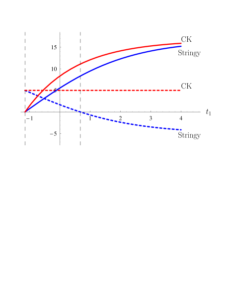
Figure 3: Expectation values of position (solid color lines) and momentum (dashed color lines) as functions of time for the Gaussian wave packet (the best fit for the moving classical particle), drawn for the stringy and CK propagators (17) and (18), respectively. Initial wave packet characteristics are $\langle q\rangle(t_{0})=0\,\mathrm{m}$ and $\langle p\rangle(t_{0})=5\,\mathrm{m\,s^{-1}}$, and the friction constant $\kappa$ is set to $0.6\,\mathrm{s^{-1}}$. One realizes that at the time $t_{1}-t_{0}=\ln{3}\ \kappa^{-1}$ the stringy mean momentum becomes zero. Classically, for $t_{1}-t_{0}>\kappa^{-1}$ the physical relevancy of the solution breaks down. This explains the time bound on the applicability of stringy propagator (17).

From the figure we can see that the stringy averaged momentum $\langle p\rangle$ becomes negative (i.e. meaningless) for $t_{1}-t_{0}>\ln{3}\ \kappa^{-1}$. Let us try to explain this peculiarity. It is well known that the relevancy of the classical solution $q_{cl}(t)$ of $\ddot{q}=-\kappa\dot{q}$ breaks down when the time $t_{1}-t_{0}$ exceeds the relaxation time $\kappa^{-1}$. Since $q_{cl}$ is used in the derivation of the formula (17) for the stringy propagator, its applicability is automatically restricted as well. After this restriction is taken into account, the stringy evolution of $\langle p\rangle$ becomes more acceptable from the physical point of view then the evolution in the CK approach.

V.2 Stringy versus Bateman approach

The key element of the Bateman(-Morse-Feshbach) approach bateman are new subsidiary degrees of freedom introduced in addition to the initial ones, which are amplified rather than damped; thus, they evolve according to the time reversed dynamical equations. In our case we have:

$$\ddot{q}=-\kappa\dot{q}\ \ \mbox{(damped) \ AND}\ \ \ddot{Q}=+\kappa\dot{Q}\ \ \mbox{(amplified)}\,.$$

These equations of motion can be derived from the least action principle with the quadratic and time independent Bateman(-Morse-Feshbach) Lagrangian:

$$L_{B}(q,\dot{q},Q,\dot{Q})=\dot{q}\dot{Q}+\frac{\kappa}{2}(q\dot{Q}-Q\dot{q})\,.$$ (19)

The canonical as well as path integral quantization of the theory encounters various difficulties because non-normalizable states of the amplified system must be employed ghosh-hasse . This problem will be discussed later, when the treatment of the auxiliary $Q$-degrees of freedom in this approach will be described. The path integral evaluation of the transition probability amplitude based on $L_{B}$ is straightforward chetouani . The result is:

$$\mathbf{A}_{B}(q_{1},Q_{1},t_{1}|q_{0},Q_{0},t_{0})=\frac{\kappa}{4\pi\hslash\sinh{\frac{\kappa T}{2}}}\times$$

$$\times\exp\Bigl{\{}\frac{i}{\hslash}\alpha\bigl{[}Q_{1}(q_{1}-q_{0}\beta_{-})+Q_{0}(q_{0}-q_{1}\beta_{+})\bigr{]}\Bigr{\}}\,,$$ (20)

where

$$\alpha=\frac{\kappa}{2}\,\frac{1}{\tanh{\frac{\kappa T}{2}}}\,,\ \ \ \beta_{\pm}=\frac{\mathrm{e}^{\pm\frac{\kappa T}{2}}}{\cosh{\frac{\kappa T}{2}}}\,,\ \ \ T=t_{1}-t_{0}\,.$$

Our aim, however, is to find the transition amplitude for the damped (sub)system only. In order to obtain it we must project out the nonphysical $Q$-degrees of freedom. When using the standard formula

$$\mathbf{A}_{B}^{\mathrm{trial}}(q_{1},t_{1}|q_{0},t_{0})=\int dQA_{B}(q_{1},Q,t_{1}|q_{0},Q,t_{0})\,,$$

we do not reproduce the free particle propagator for $\kappa=0$ as desired. To overcome this trouble the following “repairing prescription” is introduced (for more detail see nemes-toledo piza ): the amplitude for the damped (sub)system to pass from $|q_{0}\rangle$ to $|q_{1}\rangle$ within the time $T$ is equal to the amplitude for the whole system to pass from the nonphysical state $|q_{0}\rangle|\Psi_{-}\rangle$ to the nonphysical state $|q_{1}\rangle|\Psi_{+}\rangle$,

$$\mathbf{A}_{B}^{\mathrm{eff}}(q_{1},t_{1}|q_{0},t_{0}):=\mbox{Amp}\Bigl{(}|q_{0}\rangle|\Psi_{-}\rangle\rightarrow|q_{1}\rangle|\Psi_{+}\rangle\Bigr{)}=$$

$$=\int dQdQ^{\prime}\,\overline{\Psi}_{+}(Q^{\prime})\,A_{B}(q_{1},Q^{\prime},t_{1}|q_{0},Q,t_{0})\,\Psi_{-}(Q)\,,$$ (21)

where the non-normalizible $Q$-system states $|\Psi_{\pm}\rangle$ are chosen as

$$\Psi_{\pm}(Q)=\sqrt{i\cosh{\tfrac{\kappa}{2}T}\sqrt{\frac{\mp 2i\alpha}{\pi\hslash}}}\exp\bigl{\{}\pm\frac{i}{\hslash}\alpha Q^{2}\bigr{\}}\,.$$

Substituting (V.2) into (V.2) we obtain the following effective propagator for the damped (sub)system:

$$\mathbf{A}_{B}^{\mathrm{eff}}(q_{1},t_{1}|q_{0},t_{0}):=\sqrt{\frac{\kappa}{4\pi i\hslash\tanh{\frac{\kappa}{2}T}}}\times$$

$$\times\exp\Bigl{\{}\frac{i}{\hslash}\frac{\alpha}{4}\Bigl{[}\bigl{(}q_{1}-q_{0}\beta_{-}\bigr{)}^{2}+\bigl{(}q_{0}-q_{1}\beta_{+}\bigr{)}^{2}\Bigr{]}\Bigr{\}}\,.$$ (22)

The form of the auxiliary states $|\Psi_{+}\rangle$ and $|\Psi_{-}\rangle$ guarantees that the effective Bateman propagator for the damped (sub)system satisfies the normalization condition (2).

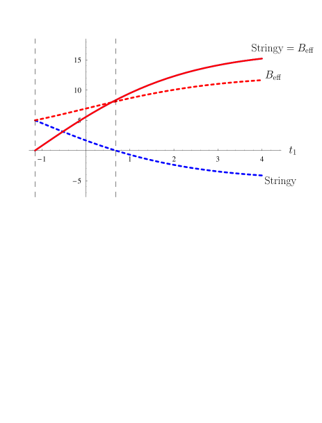
Figure 4: Expectation values of the position and momentum as functions of time for the Gaussian wave packet, drawn for the stringy and effective Bateman propagators (17) and (V.2), respectively. The initial wave packet characteristics and the meaning of solid and dashed color lines are the same as in Figure 3.

The Bateman effective propagator (V.2) depends only on the time difference $T$, which favors it in comparison with the CK-propagator (18). On the other hand, the artificial “repairing procedure” involving nonphysical states discredits the Bateman approach with respect to the stringy one. The Gaussian wave packet characteristics obtained from (17) and (V.2) are drawn in Figure 4. As seen from the figure, the stringy quantization possesses again better qualitative features than the approach to which we have compared it.

V.3 Stringy versus Kostin approach

A possible incorporation of the classical dynamics into the quantum one can be obtained by using Heisenberg equations for the position and momentum operators :

$$\dot{\hat{q}}=\hat{p}\,,\ \ \ \dot{\hat{p}}=F(\hat{q},\hat{p})\,,$$

where $\hat{q}$ and $\hat{p}$ obey $\bigl{[}\hat{q},\hat{p}\bigr{]}=i\hslash$ for all $t$. In the special case when $F(\hat{q},\hat{p})=-dU(\hat{q})/dq-\kappa\hat{p}$, Kostin found an equivalent description of the system by the Schrödinger equation kostin :

$$i\hslash\partial_{t}\Psi(q,t)=\Bigl{[}-\frac{\hslash^{2}}{2}\frac{d^{2}}{dq^{2}}+U(q)+\hslash K[\Psi]\Bigr{]}\Psi(q,t)\,,$$ (23)

where $K[\Psi]$ is the $\Psi$-dependent Kostin potential defined as

$$K[\Psi]=i\frac{\kappa}{2}\Bigl{[}\ln{\frac{\overline{\Psi}(q,t)}{\Psi(q,t)}}-\int dq^{\prime}\,\overline{\Psi}(q^{\prime},t)\ln{\frac{\overline{\Psi}(q^{\prime},t)}{\Psi(q^{\prime},t)}}\Psi(q^{\prime},t)\Bigr{]}.$$

This is known as Kostin-Schrödinger(-Langevin) equation. In the Kostin’s paper a complete set of solutions of this equation in the special case of free particle ($U(q)=0$) is presented. The set consists of the states $\Psi_{p_{0}}(q,t)$ labeled by the continuous quantum number $p_{0}$, the initial momentum of the particle. The state $\Psi_{p_{0}}(q,t)$ starts as a momentum eigenstate with the momentum $p_{0}$, and remains the momentum eigenstate also later, but with the decreasing momentum,

$$\hat{p}\Psi_{p_{0}}(q,t)=p_{0}\mathrm{e}^{-\kappa(t-t_{0})}\Psi_{p_{0}}(q,t)\,.$$

From the ensemble of non-localized Kostin’s states one would like to form normalized wave packet solutions, localized in configuration as well as momentum space. This is, however, impossible since the Kostin-Schrödinger equation is nonlinear; thus, the Kostin approach belongs to nonlinear quantum mechanics and lacks superposition principle. In Figure 5 we plot the expectation value of the momentum for the Kostin state $\Psi_{p_{0}}(q,t_{1})$ and the stringy evolved state $\Psi(q,t_{1})=\int dq^{\prime}\mathbf{A}_{1str}(q,t_{1}|q^{\prime},t_{0})\Psi_{p_{0}}(q^{\prime},t_{0})$ for various values of $\kappa$ . As $\kappa$ tends to zero, the stringy and Kostin results match each other.

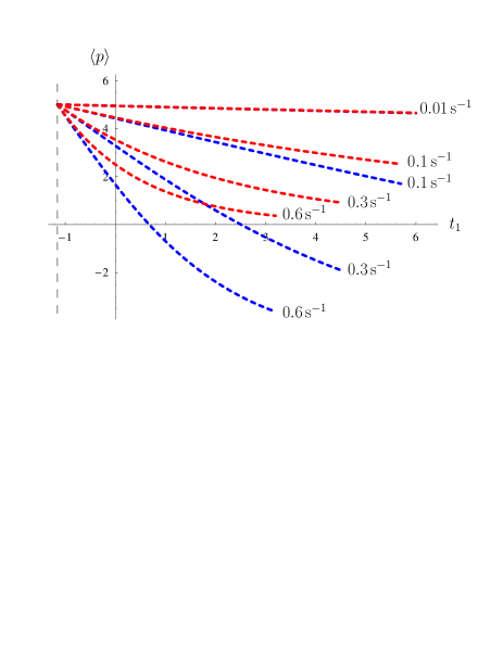
Figure 5: Expectation value of the momentum as a function of time for an eigenstate of initial momentum $\Psi_{p_{0}}(q,t_{0})\propto\exp\{\frac{i}{\hslash}qp_{0}\}$, drawn for the stringy propagator (17) (blue dashed lines) and the propagator given by the Kostin-Schrödinger equation (23) (red dashed lines), respectively. The values of the friction constant $\kappa$ are indicated next to the curves. The initial momentum is $p_{0}=5\,\mathrm{m\,s^{-1}}$.

VI Quantization of the Douglas system

After we have dealt with the weak non-Lagrangeanity, let us consider the simplest strongly non-Lagrangian system. It was proposed by Jesse Douglas (one of the two winners of the first Fields Medals awarded in 1936) when studying the inverse problem of variational calculus douglas . The system is governed by the following dimensionless dynamical equations:

$$\ddot{x}=-\dot{y},\ \ \ddot{y}=-y\ \ \ \Longleftrightarrow\ \ \ {p_{x}=\dot{x},\atop p_{y}=\dot{y},}\ \ \ {\dot{p}_{x}=-p_{y},\atop\dot{p}_{y}=-y\,.}$$ (24)

A quick calculation shows that the associated two-form

$$\Omega=d\bigl{(}p_{x}dx+p_{y}dy-\frac{p^{2}_{x}}{2}dt-\frac{p^{2}_{y}}{2}dt-\frac{y^{2}}{2}dt\bigr{)}-p_{y}dx\wedge dt$$

does not possess a non-trivial local integrator $f$. Consequently, equations (24) cannot be obtained as Euler-Lagrange (Hamilton) equations.

From the standard point of view, this curious situation is stalemate: no Lagrangian $\Rightarrow$ no Quantum Mechanics. However, the surface integral method offers a way to overcome this deadlock. Using the stringy functional integration in the extended phase space we get

$$\int\limits_{\mathscr{U}_{\gamma_{cl}}}[\mathscr{D}\Sigma]\exp{\Bigl{\{}\frac{i}{\hslash}\int\limits_{\Sigma}\Omega\Bigr{\}}}\propto$$

$$\propto\exp{\Bigl{\{}-\frac{i}{\hslash}\int\limits_{t_{0}}^{t_{1}}\bigl{(}\tfrac{1}{2}\dot{x}_{cl}^{2}+\tfrac{1}{2}\dot{y}_{cl}^{2}-\tfrac{1}{2}y_{cl}^{2}-x_{cl}p_{ycl}\bigr{)}dt\Bigr{\}}}\times$$

$$\times\int[\mathscr{D}x\,\mathscr{D}y]\exp{\Bigl{\{}\frac{i}{\hslash}\int\limits_{t_{0}}^{t_{1}}\bigl{(}\tfrac{1}{2}\dot{x}^{2}+\tfrac{1}{2}\dot{y}^{2}-\tfrac{1}{2}y^{2}-xp_{ycl}\bigr{)}dt\Bigr{\}}}.$$ (25)

Here, obviously, $(x_{cl}(t),p_{xcl}(t))$ and $(y_{cl}(t),p_{ycl}(t))$ stand for the classical solutions of (24) matching the initial and final endpoints for which the quantum transition probability amplitude is sought for, $x_{cl}(t_{0})=x_{0}$, $y_{cl}(t_{0})=y_{0}$ and $x_{cl}(t_{1})=x_{1}$, $y_{cl}(t_{1})=y_{1}$. In the classical limit $\hslash\rightarrow 0$ we want the stringy propagator (9) to maintain the properties of the original dynamical system. This guides us to define:

$$\mathbf{S}_{Dcl}(x_{1},y_{1},t_{1}|x_{0},y_{0},t_{0})=\int\limits_{t_{0}}^{t_{1}}\bigl{(}\tfrac{1}{2}\dot{x}_{cl}^{2}+\tfrac{1}{2}\dot{y}_{cl}^{2}-\tfrac{1}{2}y_{cl}^{2}-x_{cl}p_{ycl}\bigr{)}dt\,.$$

The exponential $\exp\{\frac{i}{\hslash}\mathbf{S}_{Dcl}\}$ of the classical action defined in such a way cancels the prefactor in (VI). Finally we arrive at the following transition amplitude for the Douglas system:

$$\mathbf{A}_{D}(x_{1},y_{1},t_{1}|x_{0},y_{0},t_{0})=\frac{1}{\mathbf{N}_{D}}\times$$

$$\times\int[\mathscr{D}x\mathscr{D}y]\exp{\Bigl{\{}\frac{i}{\hslash}\int\limits_{t_{0}}^{t_{1}}\bigl{(}\tfrac{1}{2}\dot{x}^{2}+\tfrac{1}{2}\dot{y}^{2}-\tfrac{1}{2}y^{2}-xp_{ycl}\bigr{)}dt\Bigr{\}}}.$$ (26)

The path integral in the configuration space we have constructed is quadratic and hence can be computed explicitly. The normalized transition amplitude is

$$\mathbf{A}_{D}(x_{1},y_{1},t_{1}|x_{0},y_{0},t_{0})=\frac{\mbox{\large{e}}^{\frac{i}{\hslash}\mathbf{S}_{Dcl}}}{2\pi i\hslash}\,\left|\begin{array}[]{cc}\dfrac{\partial^{2}\mathbf{S}_{Dcl}}{\partial x_{1}\,\partial x_{0}}&\dfrac{\partial^{2}\mathbf{S}_{Dcl}}{\partial x_{1}\,\partial y_{0}}\\ \vspace{-2mm}\hfil\\ \dfrac{\partial^{2}\mathbf{S}_{Dcl}}{\partial y_{1}\,\partial x_{0}}&\dfrac{\partial^{2}\mathbf{S}_{Dcl}}{\partial y_{1}\,\partial y_{0}}\end{array}\right|^{\frac{1}{2}},$$

where

$$\mathbf{S}_{Dcl} = \frac{(x_{1}-x_{0})^{2}}{2(t_{1}-t_{0})}+\tan^{2}{\left(\frac{t_{1}-t_{0}}{2}\right)}\,\frac{(y_{1}+y_{0})^{2}}{2(t_{1}-t_{0})}$$

$$+ \frac{\tan{\left(\frac{t_{1}-t_{0}}{2}\right)}}{(t_{1}-t_{0})}\,(x_{1}-x_{0})(y_{1}+y_{0})-(x_{1}y_{1}-x_{0}y_{0})$$

$$+ \frac{3}{4\sin{(t_{1}-t_{0})}}\bigl{[}(y_{1}^{2}+y_{0}^{2})\cos{(t_{1}-t_{0})}-2y_{1}y_{0}\bigr{]}$$

$$- \frac{(t_{1}-t_{0})}{4\sin^{2}{(t_{1}-t_{0})}}\bigl{[}(y_{1}^{2}+y_{0}^{2})-2y_{1}y_{0}\cos{(t_{1}-t_{0})}\bigr{]}\,.$$

VII Conclusion, discussion and outlook

In the paper we have developed a new quantization method that generalizes the conventional path integral approach. Throughout the paper we considered only the nonrelativistic quantum mechanics of spinless systems. However, the generalization to the field theory is rather straightforward. We have just to pass from the space of particle positions to the space of field configurations.

The mathematical language of our exposition respects the Vladimir Arnoľd “principle of minimal generality.” Formulas are mostly written down in one (local) chart. From this, however, one can ascend to a global, coordinate free description employing bundles and jet prolongations. In order that we did not cloud up the main idea of the paper, we did not follow such fluffy approach. However, in the future it could be useful to analyze obstructions to the implementation of our method which arise from the global properties of the underlying space-time geometry.

Special attention was paid to the stringy quantization of dissipative systems and of the Douglas system. The latter cannot be quantized by any known quantization technique while the former can. In fact, dissipative (friction force) systems were studied extensively in the past and several approaches to their quantization were proposed. The stringy quantization was compared with three of them, Caldirola-Kanai, Bateman and Kostin, and it was shown that it either gives better results (in the first two cases) or is simpler to apply (in the third case).

VII.1 Stringy versus Caldeira-Leggett model

As mentioned in the introduction, the quantization proposed here shares a common property with the well established approaches of Caldirola-Kanai, Bateman, Kostin and others: they all fail to cover decoherence phenomena. On the other hand, as we have seen, the stringy quantization produces a quantum propagator that does not respect the memoryless Chapman-Kolmogorov equation. We believe that this essential feature of the theory is measuring/reflecting the non-Lagrangeanity of the system on the quantum level.

From the author’s point of view one can rise a conceptual objection also against the particle-plus-environment model by Caldeira and Leggett particle+environment . Their approach is microscopical except the way in which the spectral density $\rho_{D}(\omega)$ for the reservoir degrees of freedom is introduced. This density is not obtained from any kind of microscopical theory and the form it assumes is motivated solely by the necessity to obtain the dissipative term $-\kappa\dot{q}$ in the effective theory. On the top of it, the interaction Hamiltonian is such that it produces, after integrating out the reservoir degrees of freedom, an additional Langevin stochastic force $F(t)$. Thus, the effective classical motion of the particle is governed by the Brownian equation of motion $\dot{p}=-\kappa p+F(t)$, which is conceptually different from the physical situation considered in section V. It is also worth to point out that the Caldeira-Leggett model cannot describe satisfactorily the friction force proportional to $-p^{A}$ with $A\neq 1$. There is no doubt that for $A=1$ the model gives better results than all effective theories mentioned before including the stringy one, but it is fair to say that it describes a different physical phenomenon, namely the quantum Brownian motion of a particle which is in thermal equilibrium with a reservoir.

VII.2 Surface functional integral versus Feynman-Vernon

The goal of our paper was to write down a functional integral formula for the quantum transition amplitude in terms of the underlying classical equation of motion. However, we did not eliminate the artificial notions of pure states and classical action for non-Lagrangian systems. In the surface functional integral (9), these notions were implicitly present.

A possible alternative to our approach consists in expressing the transition probability (not the probability amplitude!) using the functional integral. The probability that the system evolves from the mixed state $\rho_{{}_{0}}(q_{0},q_{0}^{\prime},t_{0})$ at the time $t_{0}$ to the mixed state $\rho_{{}_{1}}(q_{1},q_{1}^{\prime},t_{1})$ at some later time $t_{1}$ is

$$\mathbf{P}_{\rho_{{}_{0}}\rightarrow\rho_{{}_{1}}} \propto \int dq_{0}dq_{0}^{\prime}dq_{1}dq_{1}^{\prime}\rho_{{}_{0}}(q_{0},q_{0}^{\prime},t_{0})\rho_{{}_{1}}(q_{1},q_{1}^{\prime},t_{1})\times$$

$$\times \int[\mathscr{D}\tilde{\gamma}][\mathscr{D}\tilde{\gamma}^{\prime}]\exp\Bigl{\{}\frac{i}{\hslash}\Bigl{(}\int\limits_{\tilde{\gamma}}-\int\limits_{\tilde{\gamma}^{\prime}}\Bigr{)}(pdq-Hdt)\Bigr{\}}\,.$$

Here $\tilde{\gamma}$ and $\tilde{\gamma}^{\prime}$ are curves in the extended phase space whose $q$-projections connect $q_{0}$ with $q_{1}$ and $q_{0}^{\prime}$ with $q_{1}^{\prime}$ respectively. Using the Stokes theorem one is able to convert the difference of the line integrals of the one-form $pdq-Hdt$ into the surface integral of the two-form $\Omega=d(pdq-Hdt)$. Explicitly,

$$\Bigl{(}\int\limits_{\tilde{\gamma}}-\int\limits_{\tilde{\gamma}^{\prime}}\Bigr{)}pdq-Hdt=-\int\limits_{\Sigma}\Omega-\Bigl{(}\int\limits_{\lambda_{1}}-\int\limits_{\lambda_{0}}\Bigr{)}pdq\,,$$ (27)

where $\Sigma$ represents again a map from the parametric space $(t,s)\in[t_{0},t_{1}]\times[0,1]$ to the extended phase space,

$$\Sigma:(t,s)\mapsto\Sigma(t,s)\equiv\bigl{(}q_{\Sigma}(t,s),p_{\Sigma}(t,s),t_{\Sigma}(t,s)=t\bigr{)}\,,$$

such that $\partial\Sigma=\tilde{\gamma}^{\prime}(t)-\lambda_{1}(s)-\tilde{\gamma}(t)+\lambda_{0}(s)$. The sideways $\lambda$-boundary curves of $\Sigma$

$$\lambda_{0}(s)\equiv\Sigma(t_{0},s)\ \ \ \ \mbox{and}\ \ \ \ \lambda_{1}(s)\equiv\Sigma(t_{1},s)$$

live in the instant phase spaces of $\mathbb{R}^{2n+1}[q^{a},p_{a},t]$, i.e. in the submanifolds $\mathbb{R}^{2n}[q^{a},p_{a},t_{0}]$ and $\mathbb{R}^{2n}[q^{a},p_{a},t_{1}]$. Moreover, as the intrinsic parameter $s$ varies from $0$ to $1$, the $q_{\Sigma}$-components of $\lambda_{0}(s)$ and $\lambda_{1}(s)$ vary from $q_{0}$ to $q_{0}^{\prime}$ and from $q_{1}$ to $q_{1}^{\prime}$ respectively.

Let us denote by $\mathscr{U}$ the space of all $\Sigma$-maps for which

$${q_{\Sigma}(t_{0},0)=q_{0},\atop q_{\Sigma}(t_{0},1)=q_{0}^{\prime},}\ \ {q_{\Sigma}(t_{1},0)=q_{1},\atop q_{\Sigma}(t_{1},1)=q_{1}^{\prime},}\ \ {\lambda_{0}(s)\subset\mathbb{R}^{2n}[q,p,t_{0}],\atop\lambda_{1}(s)\subset\mathbb{R}^{2n}[q,p,t_{1}].}$$

Since the right hand side of (27) depends only on $\Sigma$ and its two boundaries, the double path integral $\int[\mathscr{D}\tilde{\gamma}][\mathscr{D}\tilde{\gamma}^{\prime}]\cdots$ entering $\mathbf{P}_{\rho_{{}_{0}}\rightarrow\rho_{{}_{1}}}$ can be rewritten as a surface functional integral $\int[\mathscr{D}\Sigma]\cdots$,

$$\vspace{5mm}\mathbf{P}_{\rho_{{}_{0}}\rightarrow\rho_{{}_{1}}} \propto \int dq_{0}dq_{0}^{\prime}dq_{1}dq_{1}^{\prime}\rho_{{}_{0}}(q_{0},q_{0}^{\prime},t_{0})\rho_{{}_{1}}(q_{1},q_{1}^{\prime},t_{1})\times$$ (28)

$$\times \int\limits_{\mathscr{U}}[\mathscr{D}\Sigma]\exp\Bigl{\{}-\frac{i}{\hslash}\Bigl{[}\int\limits_{\Sigma}\Omega+\Bigl{(}\int\limits_{\lambda_{1}}-\int\limits_{\lambda_{0}}\Bigr{)}pdq\Bigr{]}\Bigr{\}}\,.$$

The formula we have just arrived at was derived under the assumption that $\Omega=d(pdq-Hdt)$. However, it is clear that the expression in the exponent is free of any reference to the Hamiltonian and requires just the classical equations of motion. Therefore it seems reasonable to postulate the probability formula (28) also for non-Lagrangian systems.

The approach we shortly presented here does not use the notion of pure states of a non-Lagrangian system. It resembles the Feynman-Vernon approach feynman-vernon , in which one introduces the influence functional in the presence of dissipative forces. Our probability formula (28) uses the surface functional integral in the extended phase space, while in the Feynman-Vernon approach one just has to calculate a double path integral in the configuration space. There is a chance that after a certain discretization we will be able to convert the surface functional integral into the double path integral in the configuration space (see appendix B), and as a result, we will find the explicit form of the influence functional. Work on this topic is in progress.

$\mathscr{A.}$      $\mathscr{M.}$      $\mathscr{D.}$      $\mathscr{G.}$

Appendix A Stringy variational principle

In section III we shortly outlined how the transition amplitude (9) can be related to the stringy variational principle, with the action $\mathscr{S}$ defined in (11). In what follows we will perform a complete variation of $\mathscr{S}$, with the domain extended from $\mathscr{U}_{\gamma_{cl}}$ to a wider class $\mathscr{U}:=\bigcup_{\tilde{\gamma}_{0}}\bigcup_{\tilde{\gamma}_{1}}\mathscr{U}_{(\tilde{\gamma}_{1},\tilde{\gamma}_{0})}$. The stringy set $\mathscr{U}$ contains all surfaces in the extended phase space trapped between the submanifolds with fixed $(q_{0},t_{0})$ and $(q_{1},t_{1})$ (including separate histories, regarded as shrunk surfaces). In the course of variation the classical dynamics (5) we have started from will be recovered.

Suppose we have an extremal surface $\Sigma_{ext}\in\mathscr{U}_{(\tilde{\gamma}_{1},\tilde{\gamma}_{0})}\subset\mathscr{U}$ and a variational vector field $W$ defined in its neighborhood such that the flow of $W$ preserves $\mathscr{U}$. By definition, $W$ moves $\Sigma_{ext}\in\mathscr{U}_{(\tilde{\gamma}_{1},\tilde{\gamma}_{0})}$ to some other worldsheet $\Sigma_{ext}^{\delta W}\in\mathscr{U}_{(\tilde{\gamma}_{1}^{{}_{{}^{\prime}}},\tilde{\gamma}_{0}^{{}_{{}^{\prime}}})}$, where $\delta$ is an infinitesimal increment of the parameter of the flow generated by $W$. The situation is depicted schematically in Figure 6.

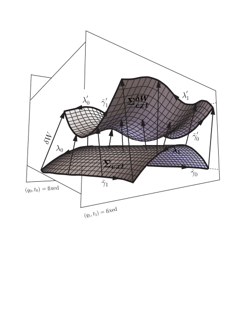
Figure 6: Vector field $W$ acting infinitesimally in the extended phase space. As a result, the initial surface $\Sigma_{ext}\in\mathscr{U}_{(\tilde{\gamma}_{1},\tilde{\gamma}_{0})}$ moves to some nearby surface $\Sigma_{ext}^{\delta W}\in\mathscr{U}_{(\tilde{\gamma}_{1}^{{}_{{}^{\prime}}},\tilde{\gamma}_{0}^{{}_{{}^{\prime}}})}$, and its boundary $\partial\Sigma_{ext}=\tilde{\gamma}_{1}-\lambda_{1}-\tilde{\gamma}_{0}+\lambda_{0}$ is transported to a new boundary $\partial\Sigma_{ext}^{\delta W}=\tilde{\gamma}_{1}^{{}_{{}^{\prime}}}-\lambda_{1}^{{}_{{}^{\prime}}}-\tilde{\gamma}_{0}^{{}_{{}^{\prime}}}+\lambda_{0}^{{}_{{}^{\prime}}}$. Since the variational vector field is assumed to preserve $\mathscr{U}$, $W$ stays tangential to the momentum submanifolds with fixed $(q_{0},t_{0})$ and $(q_{1},t_{1})$.

The extremality of $\Sigma_{ext}$ means that for all variational $W$-fields it holds

$$0=\lim\limits_{\delta\rightarrow 0}\frac{\mathscr{S}\bigl{(}\Sigma_{ext}^{\delta W}\bigr{)}-\mathscr{S}\bigl{(}\Sigma_{ext}\bigr{)}}{\delta}=\int\limits_{\Sigma_{ext}}\mathcal{L}_{W}\Omega\,,$$

where $\mathcal{L}_{W}$ stands for the Lie derivative. Let us compute the surface integral on the left hand side:

$$\int\limits_{\Sigma_{ext}}\mathcal{L}_{W}\Omega=\int\limits_{\Sigma_{ext}}d\bigl{(}W\lrcorner\,\Omega\bigr{)}+W\lrcorner\,d\Omega=$$

$$\hskip 28.45274pt=\int\limits_{\partial\Sigma_{ext}}W\lrcorner\,\Omega+\int\limits_{\Sigma_{ext}}W\lrcorner\,d\Omega\,,$$ (29)

where the the symbol $\lrcorner$ denotes the inner product (contraction) of a vector with a differential form. The first term on the right hand side depends only the values of $\Omega$ on the boundary of $\Sigma_{ext}$ and can be recast into the form

$$\int\limits_{\partial\Sigma_{ext}}W\lrcorner\,\Omega=\Bigl{(}\int\limits_{\tilde{\gamma}_{1}}-\int\limits_{\tilde{\gamma}_{0}}+\int\limits_{\lambda_{0}}-\int\limits_{\lambda_{1}}\Bigr{)}\,W\lrcorner\,\Omega\,.$$

The last two terms here give individually zero contributions, as can be seen from the following quick consideration: the vector field $W$ is assumed to preserve $\mathscr{U}$ and therefore its restrictions to the $\lambda$-boundaries are

$$W\bigr{|}_{\lambda_{0}}=W_{a}\bigl{(}p,q_{0},t_{0}\bigr{)}\frac{\partial}{\ \partial_{p_{a}}}\,,\ \ \ W\bigr{|}_{\lambda_{1}}=W_{a}\bigl{(}p,q_{1},t_{1}\bigr{)}\frac{\partial}{\ \partial_{p_{a}}}.$$

The one-form we are integrating is $W\lrcorner\,\Omega=W_{a}\bigl{(}dq^{a}-(p^{a}/m)dt\bigr{)}$, but since both $q$ and $t$ stay unchanged on $\lambda$, the integral is zero. As a result, to annihilate the boundary term for all variational fields $W$ we are forced to chose the curves $\tilde{\gamma}_{0}=(\tilde{q}_{0}(t),\tilde{p}_{0}(t),t)$ and $\tilde{\gamma}_{1}=(\tilde{q}_{1}(t),\tilde{p}_{1}(t),t)$ in the extended phase space in such a way that their instant tangent vectors annihilate $\Omega$ at any moment $t\in[t_{0},t_{1}]$. Thus, it must hold

$$0=\frac{d\tilde{\gamma}}{dt}\lrcorner\,\Omega\,,$$ (30a)

or, equivalently,

$$0=(F_{a}-\dot{p}_{a})dq^{a}+\left(\dot{q}^{a}-\frac{p^{a}}{m}\right)dp_{a}+$$

$$\hskip 48.36958pt+\left(\dot{q}^{a}F_{a}-\dot{p}_{a}\frac{p_{a}}{m}\right)dt\,,$$ (30b)

for both ${\tilde{\gamma}_{0}}$ and ${\tilde{\gamma}_{1}}$. Here one recognizes the dynamical equations (5) as desired.

From the boundary term analysis and the assumption about the uniqueness of the history $\gamma_{cl}$ which we adopted from the very beginning we can conclude that $\Sigma_{ext}\in\mathscr{U}_{(\gamma_{cl},\gamma_{cl})}\subset\mathscr{U}_{\gamma_{cl}}$. Hence $\Sigma_{ext}$ has the topology of a closed string attached to the classical trajectory $\gamma_{cl}$. To specify its shape the second term in (A) must be employed. The resulting variational equation, written in a coordinate-free notation, is

$$0=d\Omega\,\bigl{(}\partial_{t}\,\Sigma_{ext},\,\partial_{s}\,\Sigma_{ext},\,.\,\bigr{)}\,.$$ (31a)

This is equivalent to the following system of partial differential equations for the unknown functions $$q^{a}(t,s) p_{a}(t,s) a k 1,\dots,n$$ and (indices and run from ):

$$0 =\frac{\partial q^{k}}{\partial s}\,\frac{\partial F_{k}}{\partial p_{a}}\,,$$ (31b)

$$0 =\frac{\partial q^{k}}{\partial s}\,\Bigl{(}\frac{\partial F_{a}}{\partial q^{k}}-\frac{\partial F_{k}}{\partial q^{a}}\Bigr{)}+\frac{\partial p_{k}}{\partial s}\,\frac{\partial F_{a}}{\partial p_{k}}\,.$$

One solution of these equations, satisfying all boundary conditions, is trivial. It is the shrunk surface $\Sigma_{ext}(t,s)=\gamma_{cl}(t)$. After recalling the assumption of uniqueness of $\gamma_{cl}$ once more, we can see that this is the only solution of (31). If there existed a closed unshrunk extremal surface $\Sigma_{ext}$, the initial set of equations of motion (5) would have at least one one-parametrical family of classical solutions between the given pair of endpoints.

The variational principle we described above operates on a wider stringy class $\mathscr{U}$ than it is in fact necessary. The surface integral formula (9) requires just the restricted subset $\mathscr{U}_{\gamma_{cl}}\subset\mathscr{U}$. The transition to $\mathscr{U}_{\gamma_{cl}}$ is advisable for two reasons. First, in the Lagrangian case with $\Omega=d(pdq-Hdt)$ we obtain an equivalence (modulo additive constant) between the least action principle using $\mathscr{S}$ and the standard Hamilton least action principle. Explicitly,

$$\Sigma\in\mathscr{U}_{(\tilde{\gamma},\gamma_{cl})}\subset\mathscr{U}_{\gamma_{cl}}\mapsto\mathscr{S}(\Sigma)=\Bigl{(}\,\int\limits_{\tilde{\gamma}}-\int\limits_{\gamma_{cl}}\,\Bigr{)}(pdq-Hdt)\,.$$

Second, the wider class $\mathscr{U}$ contains plenty of degenerate (shrunk) surfaces, the histories $\tilde{\gamma}$. These are obviously stationary surfaces of $\mathscr{S}$ when being varied within $\mathscr{U}$, since

$$\mathscr{S}(\tilde{\gamma}^{\delta W})-\mathscr{S}(\tilde{\gamma})=\int\limits_{\tilde{\gamma}^{\delta W}}\Omega\,-\int\limits_{\tilde{\gamma}}\Omega=0-0=0$$

for any variational vector field $W$. However, only one of these histories, namely $\gamma_{cl}$, satisfies both equations (30) and (31) at the same time. This fictitious problem is avoided when one works from the beginning with the stringy subclass $\mathscr{U}_{\gamma_{cl}}\subset\mathscr{U}$.

Appendix B Surface functional integral – computational details

Let us explain here in some detail how the surface functional integral is computed. To be as tangible as possible consider a one-dimensional system only, so that the extended phase space will be the three dimensional space $\mathbb{R}^{3}[q,p,t]$ (more dimensions represent only a technical problem). The particle is supposed to move under the combined action of the potential $U(q)$ and the friction force with a general $A$-power law. The dynamical equations are

$$\dot{q}=p\,,\ \ \dot{p}=-\frac{d}{dq}U(q)-\kappa\,\dot{p}^{A}\,,$$

and in addition to them, we require that the particle satisfies the boundary conditions $q(t_{0})=q_{0}$ and $q(t_{1})=q_{1}$. According to the definition (8), the two-form $\Omega$ is

$$\Omega=d\bigl{(}pdq-\frac{1}{2}p^{2}dt-U(q)dt\bigr{)}-\kappa\,p^{A}dq\wedge dt\,.$$ (32)

Our aim is to compute the surface functional integral (9) over the stringy set $\mathscr{U}_{\gamma_{cl}}=\bigcup_{\tilde{\gamma}}\mathscr{U}_{(\tilde{\gamma},\gamma_{cl})}$. The direct application of (10) and (32) together with the Stokes theorem yields

$$\int\limits_{\mathscr{U}_{\gamma_{cl}}}[\mathscr{D}\Sigma]\exp{\Bigl{\{}\frac{i}{\hslash}\int\limits_{\Sigma}\Omega\Bigr{\}}}=$$ (33)

$$=\int[\mathscr{D}\tilde{\gamma}]\exp{\Bigl{\{}\frac{i}{\hslash}\Bigl{(}\,\int\limits_{\tilde{\gamma}}-\int\limits_{\gamma_{cl}}\,\Bigr{)}\bigl{(}pdq-\frac{1}{2}p^{2}dt-U(q)dt\bigr{)}\Bigr{\}}}\times$$

$$\times\int\limits_{\ \ \ \mathscr{U}_{(\tilde{\gamma},\gamma_{cl})}}[\mathscr{D}\Sigma]\exp{\Bigl{\{}-\frac{i}{\hslash}\kappa\int\limits_{\Sigma}p^{A}dq\wedge dt\Bigr{\}}}\,.$$

The nontrivial part of this is the functional integral over the stringy subset $\mathscr{U}_{(\tilde{\gamma},\gamma_{cl})}$. As mentioned earlier, $\Sigma\in\mathscr{U}_{(\tilde{\gamma},\gamma_{cl})}$ is a map

$$\Sigma:[t_{0},t_{1}]\times[0,1]\rightarrow\mathbb{R}^{3}[q,p,t]\,,\ \ \ (t,s)\mapsto\Sigma(t,s)\,,$$

such that for $\forall t\in[t_{0},t_{1}]$ and $\forall s\in[0,1]$ there holds

$${\Sigma(t,0)=\gamma_{cl}(t)\atop\Sigma(t,1)=\tilde{\gamma}(t)\ \,}\ \ \ \ \mbox{and}\ \ \ \ {\Sigma(t_{0},s)\in\mathbb{R}^{3}[q_{0},p,t_{0}]\atop\Sigma(t_{1},s)\in\mathbb{R}^{3}[q_{1},p,t_{1}]}\,.$$ (34)

To proceed further with the functional integral in question, introduce a set of regularly distributed nodal points in the parameter space,

$$\bigl{\{}(t_{0}+\tau\,\varDelta,\sigma\,\varepsilon)\in\bigr{[}t_{0},t_{1}]\times[0,1]\}\,.$$

The points of the set are labeled by two discrete indices, the time index $\tau=0,\dots,K$ and the space index $\sigma=0,\dots L$, see Figure 7. In this way we obtain for any $\Sigma$-map from $\mathscr{U}_{(\tilde{\gamma},\gamma_{cl})}$ a discretized $(K+1)\times(L+1)$-tuple

$$\Sigma\leftrightsquigarrow\bigl{\{}\Sigma(t_{0}+\tau\varDelta,\sigma\varepsilon)\equiv\bigl{(}q_{(\tau,\sigma)},p_{(\tau,\sigma)},t_{0}+\tau\varDelta\bigr{)}\bigr{\}}_{(\tau,\sigma)=(0,0)}^{(K,L)}\,.$$

The boundary values are required to be consistent with (34). Explicitly, for all indices $\tau$ and $\sigma$ it must hold

$${q_{(\tau,0)}=q_{cl}(t_{0}+\tau\varDelta),\atop p_{(\tau,0)}=p_{cl}(t_{0}+\tau\varDelta),}\ \ \ {q_{(\tau,L)}=\tilde{q}(t_{0}+\tau\varDelta),\atop p_{(\tau,L)}=\tilde{p}(t_{0}+\tau\varDelta),}\ \ \ {q_{(0,\sigma)}=q_{0},\atop q_{(K,\sigma)}=q_{1}.}$$

The discretization of $\Sigma$ enables us to approximate the integral of $p^{A}dq\wedge dt$ as follows :

$$\fint\limits_{\Sigma} p^{A}dq\wedge dt:=\sum\limits_{\tau=0}^{K-1}\sum\limits_{\sigma=0}^{L-1}\varDelta\varepsilon\ \Bigl{\{}p^{A}_{(\tau,\sigma)}\frac{q_{(\tau,\sigma+1)}-q_{(\tau,\sigma)}}{\varepsilon}\Bigr{\}}=$$ (35)

$$= \sum\limits_{\tau=1}^{K-1}\sum\limits_{\sigma=1}^{L-1}\,\varDelta\ \bigl{\{}q_{(\tau,\sigma)}\bigl{(}\,p^{A}_{(\tau,\sigma-1)}-p^{A}_{(\tau,\sigma)}\,\bigr{)}\bigr{\}}+$$

$$+ \sum\limits_{\tau=1}^{K-1}\,\varDelta\bigl{\{}q_{(\tau,L)}\,p^{A}_{(\tau,L-1)}-q_{(\tau,0)}\,p^{A}_{(\tau,0)}\bigr{\}}\,.$$

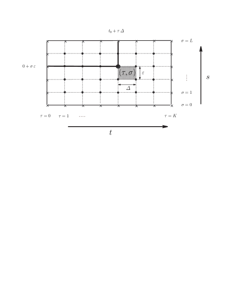
Figure 7: Rectangular nodal web in the parametric space $[t_{0},t_{1}]\times[0,1]$ of a surface $\Sigma\in\mathscr{U}_{(\tilde{\gamma},\gamma_{cl})}$. Each elementary tile encloses the area $\varDelta\cdot\varepsilon=(t_{1}-t_{0})/(KL)$ (at the end, the numbers $K$ and $L$ will be sent to infinity). The points marked by crosses are constrained by the conditions (34).

Formally, the discretized functional integral over all stringy configurations from $\mathscr{U}_{(\tilde{\gamma},\gamma_{cl})}$ is a multiple integral over all unconstrained variables $x_{(\tau,\sigma)},p_{(\tau,\sigma)}$ which are needed to specify $\Sigma$. The only problematic part, as usual, is the choice of an appropriate integration measure. For the reason that will become clear in a moment, we choose the measure as

$$\fint\limits_{\ \ \ \mathscr{U}_{(\tilde{\gamma},\gamma_{cl})}}[\mathscr{D}\Sigma]:=\int\limits_{-\infty}^{+\infty}\ \prod\limits_{\tau=1}^{K-1}\prod\limits_{\sigma=1}^{L-1}\,\Bigl{(}\frac{A\kappa\varDelta}{2\pi i\hslash}\,p^{A-1}_{(\tau,\sigma)}\Bigr{)}\,dq_{(\tau,\sigma)}\,dp_{(\tau,\sigma)}.$$ (36)

The first step, when dealing with the discretized functional integral

$$\mathrm{Int}\equiv\fint\limits_{\ \ \ \mathscr{U}_{(\tilde{\gamma},\gamma_{cl})}}[\mathscr{D}\Sigma]\exp{\Bigl{\{}-\frac{i}{\hslash}\kappa\fint\limits_{\Sigma}p^{A}dq\wedge dt\Bigr{\}}}\,,$$

consists in the integration over the internal stringy positions $dq_{(\tau,\sigma)}$. After this integration, the integrand transforms into a chain of delta functions,

$$\mathrm{Int} = \int\limits_{-\infty}^{+\infty}\prod\limits_{\tau=1}^{K-1}\prod\limits_{\sigma=1}^{L-1}\,\bigl{(}A\,p^{A-1}_{(\tau,\sigma)}\bigr{)}\,dp_{(\tau,\sigma)}\,\mbox{\large{$\bm{\delta}$}}\bigl{(}p^{A}_{(\tau,\sigma-1)}-p^{A}_{(\tau,\sigma)}\bigr{)}\times$$

$$\times \exp{\Bigl{\{}-\frac{i}{\hslash}\kappa\sum\limits_{\tau=1}^{K-1}\,\varDelta\bigl{[}q_{(\tau,L)}\,p^{A}_{(\tau,L-1)}-q_{(\tau,0)}\,p^{A}_{(\tau,0)}\bigr{]}\Bigr{\}}}\,.$$

The next step is the integration over the internal stringy momenta $dp_{(\tau,\sigma)}$. After performing this trivial integration we arrive at the expression

$$\mathrm{Int}=\exp{\Bigl{\{}-\frac{i}{\hslash}\kappa\sum\limits_{\tau=1}^{K-1}\,\varDelta\bigl{[}q_{(\tau,L)}\,p^{A}_{(\tau,0)}-q_{(\tau,0)}\,p^{A}_{(\tau,0)}\bigr{]}\Bigr{\}}}\,.$$

In the exponent there appears the discretized version of the integral

$$\int\limits_{t_{0}}^{t_{1}}\,dt\bigl{\{}\tilde{q}(t)\,p^{A}_{cl}(t)-q_{cl}(t)\,p^{A}_{cl}(t)\bigr{\}}\,,$$

where $\tilde{q}(t)$ stands for the $q$-projection of $\tilde{\gamma}(t)$. Consequently, after returning back to the continuum limit we obtain the following important result:

$$\int\limits_{\ \ \ \mathscr{U}_{(\tilde{\gamma},\gamma_{cl})}}[\mathscr{D}\Sigma]\exp{\Bigl{\{}-\frac{i}{\hslash}\kappa\int\limits_{\Sigma}p^{A}dq\wedge dt\Bigr{\}}}=$$

$$=\exp{\Bigl{\{}-\frac{i}{\hslash}\kappa\int\limits_{t_{0}}^{t_{1}}\,dt\bigl{[}\tilde{q}(t)\,p^{A}_{cl}(t)-q_{cl}(t)\,p^{A}_{cl}(t)\bigr{]}\Bigr{\}}}\,.$$ (37)

After substituting (B) into the initial formula (33) we recover a path integral in the extended phase space. The integral is quadratic in momenta, with the discretized (standard) Liouville measure

$$\fint[\mathscr{D}\tilde{\gamma}]\ \cdots=\int\limits_{-\infty}^{+\infty}\frac{d\tilde{p}_{K}}{2\pi\hslash}\,\prod\limits_{\tau=1}^{K-1}\frac{d\tilde{p}_{\tau}\,d\tilde{q}_{\tau}}{2\pi\hslash}\ \cdots\,,$$

The integration over momenta can be carried out explicitly and we finally obtain a path integral in the configuration space only (tildes are removed from the position variables),

$$\int\limits_{\mathscr{U}_{\gamma_{cl}}}[\mathscr{D}\Sigma]\exp{\Bigl{\{}\frac{i}{\hslash}\int\limits_{\Sigma}\Omega\Bigr{\}}}=$$

$$=\exp{\Bigl{\{}-\frac{i}{\hslash}\int\limits_{t_{0}}^{t_{1}}\Bigl{(}\frac{1}{2}\dot{q}_{cl}^{2}-U(q_{cl})-\kappa q_{cl}\,p^{A}_{cl}\Bigr{)}dt\Bigr{\}}}\times$$

$$\times\int[\mathscr{D}q]\exp{\Bigl{\{}\frac{i}{\hslash}\int\limits_{t_{0}}^{t_{1}}\Bigl{(}\frac{1}{2}\dot{q}^{2}-U(q)-\kappa q\,p^{A}_{cl}\Bigr{)}dt\Bigr{\}}}\,.$$ (38)

This formula served us as a guide when introducing the classical action (13).

Let us make one final comment. In our functional measure (36) no integration over the momenta $p_{(0,\sigma)}$ and $p_{(K,\sigma)}$ was prescribed. These momenta are however needed when the boundary of the discretized surface $\Sigma\in\mathscr{U}_{\gamma_{cl}}$ is specified. They define the auxiliary curves $\lambda_{0}(s)$ and $\lambda_{1}(s)$ introduced in section III. The curves were chosen completely arbitrarily, but as seen from (35), the result is not affected by them at all. Hence, since everything substantial is independent of $p_{(0,\sigma)}$ and $p_{(K,\sigma)}$, it is justifiable to discard these quantities from the functional measure $[\mathscr{D}\Sigma]$. If we would not do that for some reason, they will integrate into an artificial infinite factor, which will be removed anyway after we apply the normalization conditions (2).

References

• (1) S. T. Ali, M. Engliš: Quantization Methods: A Guide for Physicists and Analysts, Rev. Math. Phys. 17 (2005), 391-490, arXiv: math-ph/0405065.
• (2) P. Caldirola: Forze non conservative nella meccanica quantistica, Nuovo Cim. 18 (1941), 393-400. E. Kanai: On the Quantization of the Dissipative Systems, Prog. Theor. Phys. 3 (1948), 440-442.
• (3) H. Bateman: On Dissipative Systems and Related Variational Principles, Phys. Rev. 38 (1931), 815-819.
• (4) M. D. Kostin: On the Schrödinger-Langevin Equation, J. Chem. Phys. 57 (1972), 3589-3591.
• (5) H. Dekker: On the Quantization of Dissipative Systems in the Lagrange-Hamilton Formalism, Z. Phys. B 21 (1975) 295-300.
• (6) M. Razavy: On the Quantization of Dissipative Systems, Z. Physik B 26 (1977) 201-206.
• (7) J. Geicke: Semi-classical quantisation of dissipative equations, J. Phys. A: Math. Gen. 22 (1989) 1017-1025.
• (8) J. Douglas: Solution of the inverse problem in the calculus of variations, Trans. Am. Math. Soc. 50 (1941), 71-128.
• (9) A. O. Caldeira, A. J. Leggett: Path integral approach to quantum Brownian motion, Physica 121A (1983), 587-616. U. Weiss: Quantum Dissipative Systems (second edition), World Scientific 1999, Singapore.
• (10) R. P. Feynman, F. L. Vernon: The Theory of a General Quantum System Interacting with a Linear Dissipative System, Annals of Physics 24 (1963), 118-173.
• (11) F. J. Dyson: Feynman’s Proof of the Maxwell Equations, Am. J. Phys. 58 (1990), 209-211.
• (12) E. P. Wigner: Do the Equations of Motion Determine the Quantum Mechanical Commutation Relations?, Phys. Rev. 77 (1950), 711-712. C. N. Yang, D. Feldman: The S-Matrix in the Heisenberg Representation, Phys. Rev. 79 (1950), 972 - 978. E. Nelson: Derivation of the Schrödinger Equation from Newtonian Mechanics, Phys. Rev. 150 (1966), 1079-1085. S. Okubo: Does the Equation of Motion determine Commutation Relations?, Phys. Rev. D 22 (1980), 919-923.
• (13) P. O. Kazinski, S. L. Lyakhovich, A. A. Sharapov: Lagrange structure and quantization, JHEP 0507 (2005) 076, arXiv: hep-th/0506093. S. L. Lyakhovich, A. A. Sharapov: Quantizing non-Lagrangian gauge theories: an augmentation method, JHEP 0701 (2007) 047, arXiv: hep-th/0612086.
• (14) D. M. Gitman, V. G. Kupriyanov: Canonical quantization of so-called non-Lagrangian systems, Eur. Phys. J. C 50 (2007), 691-700, arXiv: hep-th/0605025.
• (15) R. P. Feynman: Space-Time Approach to Non-Relativistic Quantum Mechanics, Rev. of Mod. Phys. 20 (1948), 367-387. R. P. Feynman, A. R. Hibbs: Quantum Mechanics and Path Integrals, McGraw-Hill Inc., New York, 1965.
• (16) M. Henneaux: Equations of motion, Commutation Relations and Ambiguities in the Lagrangian Formalism, Annals Phys. 140 (1982), 45-64. M. Henneaux: On the Inverse Problem of the Calculus of Variations, J. Phys. A: Math. Gen. 15 (1982), L93-L96. W. Sarlet: The Helmholtz Condition Revisited. A New Approach to the Inverse Problem of Lagrangian Dynamics, J. Phys. A: Math. Gen. 15 (1982), 1503-1517.
• (17) D. Kochan: Direct quantization of equations of motion, Acta Polytechnica 47 No. 2-3 (2007), 60-67, arXiv: hep-th/0703073. D. Kochan: How to Quantize Forces(?): An Academic Essay on How the Strings Could Enter Classical Mechanics, J. Geom. Phys. 60 (2010), 219-229, arXiv: hep-th/0612115. D. Kochan: Quantization of Non-Lagrangian systems: some irresponsible speculations AIP Conf. Proc. 956 (2007), 3-8.
• (18) C. Stuckens, D. H. Kobe: Quantization of a particle with a force quadratic in the velocity, Phys. Rev. A 34 (1986) 3565-3567.
• (19) H. Dekker: Classical and quantum mechanics of the damped harmonic oscillator, Phys. Rep. 80 (1981), 1-112.
• (20) M. Razavy: Classical and Quantum Dissipative Systems; Imperial Colleges Press, London, 2005.
• (21) I. C. Moreira: Propagators for the Caldirola-Kanai-Schrödinger Equation, Lett. Nuovo Cim. 23 (1978), 294-298. A. D. Jannussis, G. N. Brodimas, A. Strectlas: Propagator with friction in Quantum Mechanics, Phys. Lett. 74A (1979), 6-10. Bin Kang Cheng: Exact evaluation of the propagator for the damped harmonic oscillator, J. Phys. A: Math. Gen. 17 (1984), 2475-2484. U. Das, S. Ghosh, P. Sarkar, B. Talukdar: Quantization of Dissipative Systems with Friction Linear in Velocity, Physica Scripta 71 (2005), 235-237.
• (22) D. Kochan: Quantization of Non-Lagrangian Systems, Int. J. Mod. Phys. A 24 Nos. 28 $\&$ 29 (2009), 5319-5340.
• (23) G. Ghosh, R. W. Hasse: Coherent state and the damped harmonic oscillator, Phys. Rev. A 24 (1981), 1621-1623.
• (24) L. Chetouani et al: Path integral for the damped harmonic oscillator coupled to its dual, J. Math. Phys. 35 (1994), 1185-1191.
• (25) M. C. Nemes, A. F. R. de Toledo Piza: A Quantum Phenomenology of Viscosity, Revista Brasileira de Física 7 No.2 (1977), 261-270. M. C. Nemes, A. F. R. de Toledo Piza: Quantization of a phenomenological viscous force, Phys. Rev. A 27 (1983), 1199-1202.