Quantification of the Heterogeneity of Particle Packings

Abstract

The microstructure of coagulated colloidal particles, for which the inter-particle potential is described by the DLVO theory, is strongly influenced by the particles’ surface potential. Depending on its value, the resulting microstructures are either more ”homogeneous” or more ”heterogeneous”, at equal volume fractions. An adequate quantification of a structure’s degree of heterogeneity (DOH) however does not yet exist. In this work, methods to quantify and thus classify the DOH of microstructures are investigated and compared. Three methods are evaluated using particle packings generated by Brownian dynamics simulations: (1) the pore size distribution, (2) the density fluctuation method and (3) the Voronoi volume distribution. Each method provides a scalar measure, either via a parameter in a fit function or an integral, which correlates with the heterogeneity of the microstructure and which thus allows for the first time to quantitatively capture the DOH of a granular material. An analysis of the differences in the density fluctuations between two structures additionally allows for a detailed determination of the length scale on which differences in heterogeneity are most pronounced.

I Introduction

Colloidal particle packings are suitable model systems for the study of the structural properties of granular materials below the random loose packing limit. For such systems the gravitational force is negligible in comparison to the van der Waals force, electrostatic repulsion or Brownian motion Visser (1989); Israelachvili (1991). In the present study, we particularly focus on systems, for which the local arrangement of the particles is the only variable, as opposed to variations in the volume fraction or the particle size distribution for example. Commonly, these microstructures are referred to as ”more homogeneous” or ”more heterogeneous”, which either designates a structure presenting a rather uniform distribution of the particle positions or one having locally denser regions and therefore larger voids. These qualitative terms may be intuitive, however, they do not allow for a sound scientific quantification of the structure’s degree of heterogeneity (DOH), which does not yet exist. In this paper, three methods providing the means for such a quantification are presented, analyzed and compared. These methods permit for the first time to explicitly capture the DOH of a particle packing in form of a quantitative, scalar measure.

Experimentally, the reproducible generation of colloidal particle packings possessing a specific DOH is achieved by the use of an in-situ enzyme-catalyzed destabilization method (Direct Coagulation Casting (DCC), Gauckler et al. (1999); Tervoort et al. (2004)). For volume fractions between 0.2 and 0.6, DCC allows for the coagulation of electrostatically stabilized colloidal suspensions to stiff particle structures by either shifting the pH of the suspension to the particles’ isoelectric point or by increasing the ionic strength of the suspension without disturbing the particle system. Shifting the pH leads to ”more homogeneous” microstructure through diffusion limited aggregation while increasing the ionic strength results in ”more heterogeneous” microstructures via reaction rate limited aggregation. The differences in heterogeneity have been observed using various techniques such as diffusing wave spectroscopy Wyss et al. (2001), static light transmission Wyss et al. (2001) or cryogenic scanning electron microscopy Wyss et al. (2002).

Computationally, microstructures with different DOH were successfully reproduced using Brownian dynamics simulations (BD) Wyss et al. (2002); Hütter (2000, 1999). Slices of three particle layer thickness through a ”homogeneous” and a ”heterogeneous” BD-microstructure of identical volume fraction nicely demonstrate the differences between the microstructures (Fig. 1). The microstructure on the left presents a rather uniform distribution of the particle positions over the whole slice while the microstructure on the right presents locally more densely packed particles and consequently larger voids. Both structures have an identical overall volume fraction of 0.4.

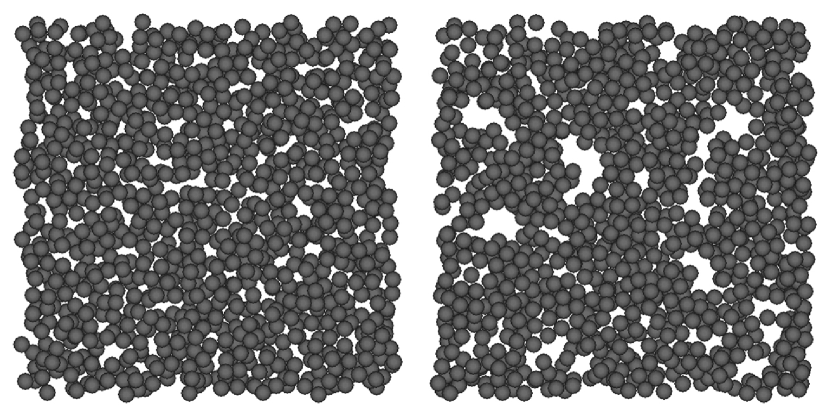
Figure 1: Slices through a ”homogeneous” (left) and a ”heterogeneous” (right) particle structure with the same volume fraction of 0.4 resulting from Brownian dynamics simulations Hütter (2000) (slice thickness: three particle diameters; particle diameter: 0.5 $\mu$m).

In preceding works, various characterization methods, such as the radial pair correlation function Hütter (2000), the bond angle distribution function Hütter (2000), the triangle distribution function Hütter (2000) and the Minkowski functionals in conjunction with the parallel-body technique Hütter (2003) were applied to sets of microstructures generated by BD simulations Hütter (1999).

The pair correlation function quantifies the amount of structural rearrangement during the coagulation. Its usefulness regarding a distinction between structures with different DOH however is rather limited as the differences between peaks corresponding to characteristic particle separation distances are relatively small Hütter (2000). The main advantage of the pair correlation function is its experimental accessibility through scattering techniques such as SESANS Andersson et al. (2008).

The bond angle distribution function and the triangle distribution function give further information on the local building blocks of the particle network Hütter (2000). Particular features, as for example peaks in the respective distribution function allow distinguishing between ”more homogeneous” and ”more heterogeneous” microstructures. However, as in the case of the pair correlation function, the differences between structures with different DOH are small for both, the bond angle and the triangle distribution function.

The analysis using the Minkowski functionals in conjunction with the parallel body technique supplies additional information on the structure’s morphology resolving microstructural differences on a length scale limited by the largest pore size Hütter (2003). This method is computationally intensive and the extension to arbitrary particle shapes is difficult.

Gearing towards a possible correlation between microstructure and mechanical properties ”homogeneous” and ”heterogeneous” microstructures have recently been analyzed in terms of load bearing sub-structures: Firstly, regions of closely packed particles and secondly, quasi-linear chains of contacting particles Schenker et al. (2008). The locally closed packed regions were analyzed using the common neighbor distribution in conjunction with the dihedral angle distribution. Both methods only showed minor differences between a ”homogeneous” and a ”heterogeneous” microstructure. In particular, practically the same number of triangles and regular tetrahedrons were found in both structures. Quasi-linear arrangements of contacting particles were quantified using the straight path method, revealing significant microstructural differences between ”homogeneous” and ”heterogeneous”: approximately twice as many paths of length longer or equal to four particles and three times as many paths of length longer or equal to five particles where found in the ”heterogeneous” microstructure.

Despite the multitude of microstructural characterization methods that have been applied to colloidal microstructures possessing various DOH, a useful quantification of the microstructures’ heterogeneity in form of a scalar measure is lacking. In the present study statistical measures allowing for a quantification of a structure’s heterogeneity are provided. The following three methods aiming at this quantification are discussed.

Firstly, the exclusion probability Torquato et al. (1990) estimates the pore size distribution by randomly probing the pore space. In Whittle and Dickinson (1999) this method was applied to very dilute simulated colloidal systems and allowed for a clear distinction between particle gel networks with varying textures. The same method, termed spherical contact distribution function Bezrukov et al. (2002), was used to investigate the pore size distribution of dense sphere packings as a function of the particle size distribution and the packing generation algorithm.

Secondly, the density fluctuation method considers the fixed particle centers as a point process, and it statistically analyses the fluctuations of the particle center density as a function of length scale. Used comparatively, this method further allows for a detailed analysis of the length scale, on which two structures present the largest differences in terms of heterogeneity.

Finally, the Voronoi volume distribution Voronoi (1908) is used to quantify the distribution of the free volume of our particle packings. In Yang et al. (2002) the packing of cohesive particles resulting from simulations using the discrete element method Cundall and Strack (1979) with volume fractions between approximately 0.2 and 0.6 was analyzed. The distribution of Voronoi volumes was shown to broaden with decreasing volume fraction. In Aste and Di Matteo (2008) the Voronoi volume distribution was determined for a large set of experimental and numerical data covering a wide range of volume fractions. The various distributions were shown to follow a so-called $k$-gamma function, which was deduced by means of a statistical mechanics approach. The parameter $k$ characterizing the shape of the curve was found to depend very sensitively on the structural organization of the particles.

To the authors’ knowledge, none of these methods have yet been applied to particle structures, for which the DOH is the only variable, in opposition to a varying volume fraction or particle size distribution for example.

II Materials and Methods

In the following, the structure characterization methods employed in this work are presented: the pore size distribution, the density fluctuation method and the distribution of Voronoi volumes. These methods are evaluated in terms of their ability to quantify the DOH of microstructures generated by previous BD simulations Hütter (2000, 1999). In these simulations, the DLVO-theory Russel et al. (March 1989) was used to describe the inter-particle potential $V^{dlvo}$ given by the sum of an attractive van der Waals term $V^{vdw}$ (Eq. 1) and an electrostatic repulsion term $V^{el}$ (Eq. 2).Thus, $V^{dlvo}=V^{vdw}+V^{el}$ with,

$$V^{vdw}(r)=\frac{-A_{H}}{12}\left[\frac{d_{0}^{2}}{r^{2}-d_{0}^{2}}+\frac{d_{0}^{2}}{r^{2}}+2\ln\left(\frac{r^{2}-d_{0}^{2}}{r^{2}}\right)\right]$$ (1)

and

$$V^{el}(r)= \pi\epsilon_{r}\epsilon_{\mathrm{0}}\left[\frac{4k_{b}T}{ze}\tanh\left(\frac{ze}{4k_{b}T}\Psi_{\mathrm{0}}\right)\right]^{2}$$ (2)

$$\times d_{0}\exp\left(-\kappa\{r-d_{0}\}\right)$$

respectively. The DLVO parameters are summarized in Table 1.

Table 1: DLVO Potential Parameters.

Parameter	Symbol	Value
Hamaker constant of Al2O3 in H2O	$A_{H}$	$4.76\times 10^{-20}$ J
Particle diameter	$d_{0}$	5 $\times$ 10-7 m
Relative dielectric constant of H2O	$\epsilon_{r}$	81
Surface potential	$\Psi_{0}$	0 - 15 mV
Absolute temperature	$T$	293 K
Valency of ions	$z$	1
Inverse Debye screening length	$\kappa$	108 m-1

The heterogeneity of the final microstructure was shown to be closely related to the presence and depth of the secondary minimum in the inter-particle potential, which, for fixed values of the Debye screening length, essentially depends on the particles’ surface potential $\Psi_{0}$ Wyss et al. (2005); Hütter (2000).

The microstructures analyzed in this work are labelled according to the surface potential $\Psi_{0}$ used during their generation. In particular, the following $\Psi_{0}$-values are used: 0 mV, 12 mV, 13 mV, 14 mV and 15 mV. Additionally, these final microstructures are compared to the initial microstructure, representing a stabilized suspension in which the inter-particle potential is purely repulsive. The volume fraction is fixed at 0.4, the monosized particles have a radius $r_{0}$ = 0.25 $\mu$m, all microstructures consist of 8000 particles and are contained in a simulation box with periodic boundary conditions. In particular, the particle interpenetration is much smaller than the length scale of the heterogeneities analyzed in this study. Less than 0.1% of all contacts present an interpenetration above 1.0% of the particle diameter $d_{0}$ with a maximum interpenetration of 1.3% $d_{0}$. Please refer to Hütter (2000, 1999) for a more detailed description of the BD-simulations.

II.1 Pore Size Distribution

The pore size distribution is estimated following the approach described by Torquato et al. Torquato et al. (1990) using the exclusion probability $E_{V}(r)$. $E_{V}(r)$ is defined as the probability of inserting a ”test” particle of radius $r$ at some arbitrary position in the pore space of a system of $N$ particles. This is schematically represented in Fig. 2 using a set of particles of radius $r_{0}$ (gray) with a test particle of radius $r$ inserted at position $P$.

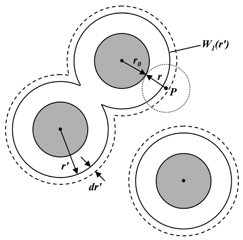
Figure 2: Particle structure (gray particles) with a test particle inserted at position $P$.

In order to estimate $E_{V}(r)$, a statistically large number of points is randomly placed in the pore space of a given microstructure and the distance to the closest particle surface is determined.

In Hütter (2003) the relation between $E_{V}(r)$ and the Minkowski functional $W_{1}(r)$ was described. The Minkowski functional in conjunction with the parallel body technique considers the point process given by the fixed particle centers. Generally, in three dimensions there are four functionals $W_{i}$, where $i=0,..,d$ with $d$ the spatial dimension, corresponding to the volume, surface, average mean curvatures and connectivity. In particular, $W_{1}(r^{\prime})=\frac{1}{3}\int_{\partial A(r^{\prime})}dS$ calculates the surface of the union of spheres located at the particle centers in dependence of their radius $r^{\prime}=r_{0}+r$. Schematically, $W_{1}(r^{\prime})$ is shown in Fig. 2. $W_{1}(r^{\prime})dr^{\prime}$ is the volume between the distance $r^{\prime}$ and $r^{\prime}+dr^{\prime}$. The probability of placing an uniformly drawn random test point at a distance $r\in[r^{\prime},r^{\prime}+dr^{\prime}[$ is proportional to the volume delimited by $r^{\prime}$ and $r^{\prime}+dr^{\prime}$ and therefore $P(r^{\prime}\leq r_{0}+r<r^{\prime}+dr^{\prime})=E_{V}(r)dr^{\prime}\propto W_{1}(r^{\prime})dr^{\prime}$, which results in $E_{V}(r_{0}+r)\propto W_{1}(r^{\prime})$. Thus, given a statistically large number of test points $E_{V}(r)$ provides a means to estimate $W_{1}(r^{\prime})$, which has the advantage of being computationally less intensive. A similar Monte Carlo integration is usually performed to calculate $W_{0}(r^{\prime})$.

II.2 Density Fluctuations

The density fluctuation method quantifies the local fluctuation of particle centers by subdividing the structure into smaller parts and measuring the average value and the standard deviation of the particle center density. Practically, this is done by dividing the structure into $n_{c}^{3}$ cells using a cubic grid, where $n_{c}$ is the number of cells along one dimension with $n_{c}$ = 2, .., $n_{c}^{max}$, $n_{c}^{max}$ being the maximum number of cells under consideration (along one dimension). The density fluctuation method consists in determining the average number of particle centers per cell $E_{ppc}$ and its standard deviation $\sigma_{ppc}$ as a function of $n_{c}$ and then calculating the relative fluctuations $\frac{\sigma_{ppc}}{E_{ppc}}$.

Additionally, the density fluctuation method is applied comparatively allowing for a determination of the length scale on which two structures show the largest differences. Therefore, the difference $\Delta(n_{c})$ given in Eq. (3) is calculated between two structures $i$ and $j$.

$$\Delta(n_{c})=\left[\frac{\sigma_{ppc}^{i}}{E_{ppc}^{i}}-\frac{\sigma_{ppc}^{j}}{E_{ppc}^{j}}\right](n_{c})$$ (3)

If both structures have the same number of particles and identical volume fractions, which is the case for the microstructures investigated in this work, then $E_{ppc}^{i}=E_{ppc}^{j}=E_{ppc}$ and Eq. (3) yields Eq. (4).

$$\Delta(n_{c})=\frac{\sigma_{ppc}^{i}-\sigma_{ppc}^{j}}{E_{ppc}}(n_{c})$$ (4)

$\Delta$ is plotted against the cell’s edge length $l_{c}(n_{c})=L_{Box}/n_{c}$ normalized by the particle diameter $d_{0}$, where $L_{Box}$ is the side length of the cubic simulation box.

II.3 Voronoi Volume Distribution

Formally, for a set of monodispersed spherical particles, the Voronoi volume $V_{i}$ associated with a particle $i$ is a polyhedron whose interior consists of all points in space that are closer to the center of particle $i$ than to any other particle center Voronoi (1908). The Voronoi tessellation thus divides the volume containing a set of particles into a set of space-filling, non-overlapping and convex polyhedrons. In this work, the Quickhull algorithm Barber et al. (1996) is used to compute the volumes of the Voronoi polyhedrons. The distribution of the Voronoi volumes describes the deviation of a structure from a perfect crystalline packing, in which case all particles occupy the same volume and the Voronoi volume distribution thus is a delta function. The minimum volume of a Voronoi cell $V_{min}$ is achieved for a regular close packing with $V_{min}=1.325V_{sphere}$, where $V_{sphere}$ is the volume of a particle. The difference between a particle’s Voronoi volume $V_{i}$ and $V_{min}$ is termed the Voronoi free volume $V_{i}^{f}=V_{i}-V_{min}$.

The distribution of the Voronoi free volume was found to follow gamma-distributions: Kumar and Kumaran for example have shown that the free volume distribution of hard-disk and hard-sphere systems are well described using a two-parameter and a three-parameter gamma-distributions Kumar and Kumaran (2005).

Aste et al. have deduced the two-parameter gamma-distribution using a statistical mechanics approach Aste and Di Matteo (2008). The so-called $k$-gamma distribution given by Eq. (5) was found to agree very well with a large number of experiments and computer simulations over a wide range of packing fractions.

$$f(V^{f},k)=\frac{k^{k}}{\Gamma(k)}\frac{(V^{f})^{k-1}}{(\bar{V}^{f})^{k}}\exp(-k\frac{V^{f}}{\bar{V}^{f}})$$ (5)

The mean Voronoi free volume $\bar{V}^{f}$ is a scaling parameter given by $\bar{V}-V_{min}=\left(1/\Phi-1.325\right)V_{sphere}$, where $\Phi$ is the volume fraction. The free parameter $k$ characterizing the shape of the curve depends very sensitively on the structural organization of the particles and corresponds to the specific heat in classical thermodynamics. Empirically, $k$ can be computed using $k=\frac{(\bar{V}^{f})^{2}}{\sigma_{V}^{2}}$, where $\sigma_{V}^{2}$ is the variance of the free volume distribution. In particular, Eq. (5) was shown to hold for systems at statistical equilibrium as well as for systems out of equilibrium Aste and Di Matteo (2008).

III Results and Discussion

III.1 Pore Size Distribution

The pore size distribution of the various microstructures is depicted in Fig. 3 in terms of the exclusion probability $E_{V}(r_{P})$ as a function of the pore radius $r_{P}$ normalized by the particle radius $r_{0}$. A set of $10^{6}$ random test points Matsumoto and Nishimura (1998) placed in the structures’ pore space was used to estimate $E_{V}(r_{P})$.

All curves for the final microstructures ($\Psi_{0}$ = 0 - 15 mV) decrease monotonically towards increasing pore sizes indicating a decreasing probability of finding larger pores. A particular behavior is found for the stable suspension where the exclusion probability increases with increasing pore size up to a pore radius of $0.18r_{0}$. This is due to the repulsive inter-particle potential in the case of the stable suspension where consequently, the particles are not in contact. The pore diameter, at which the maximum in the exclusion probability is found, corresponds to the average surface-to-surface distance between neighboring particles.

Remarkably, the various curves for the final microstructures in Fig. 3 intersect at approximately the same point defining a characteristic pore size $r_{p}^{c}$, found at $0.65r_{0}$. The probability of finding a pore with a radius below $r_{p}^{c}$ decreases for increasing values of $\Psi_{0}$ while pores with a radius above $r_{p}^{c}$ are found with higher probability towards increasing $\Psi_{0}$. Indeed, the probability of finding pore radii larger than approximately $1.1r_{0}$ is negligible in the case of the ”most homogeneous” microstructure with $\Psi_{0}$ = 0 mV while pore radii up to $2.4r_{0}$ are found in the ”most heterogeneous” microstructure with $\Psi_{0}$ = 15 mV.

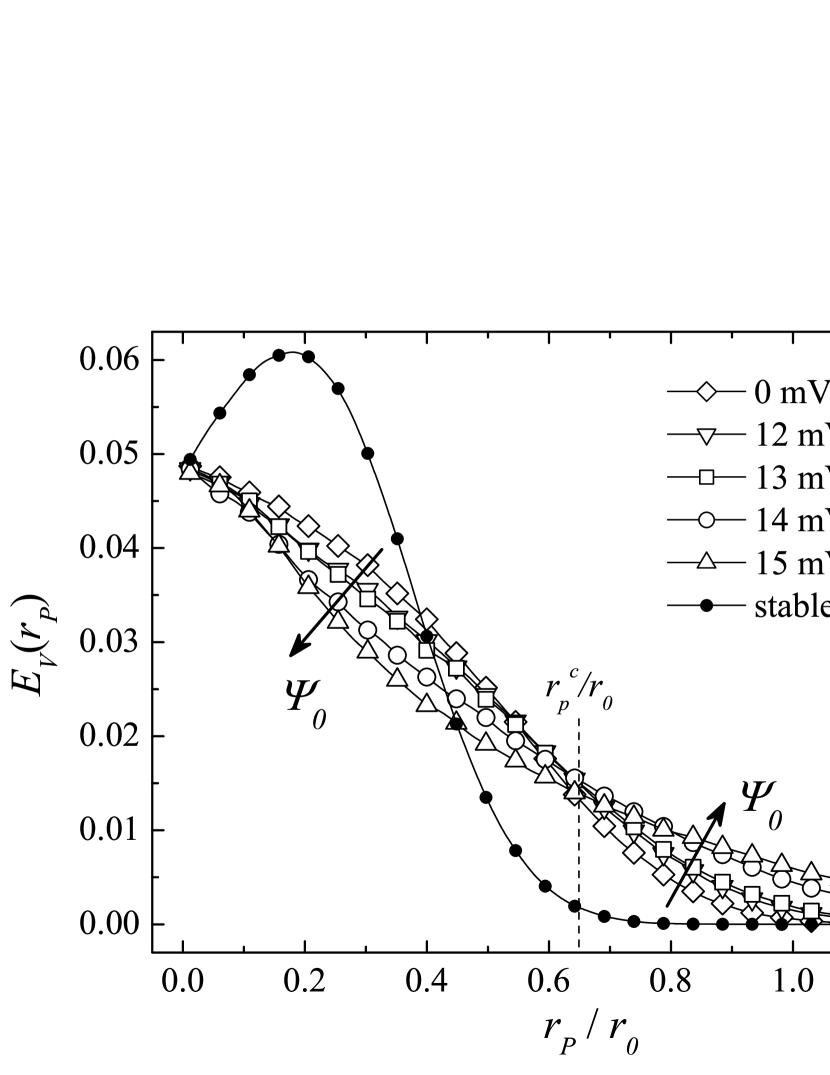
Figure 3: Pore size distribution for the initial microstructure (stable suspension) and final microstructures ($\Psi_{0}$ = 0 - 15 mV). B-spline curves serve as guide to the eye.

Using the results obtained for the exclusion probability $E_{V}(r_{P})$, the cumulative probability $P(r_{P}>r)$ of finding pore radii larger than $r$ was calculated using $P(r_{P}>r)=\sum_{r^{\prime}>r_{P}}E_{V}(r^{\prime})$. The results are shown in Fig. 4.

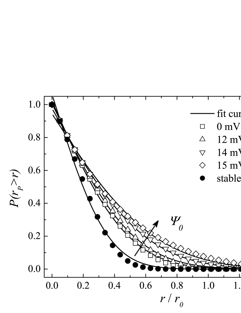
Figure 4: Probability of finding pores with a radius $r_{P}$ larger than $r$ vs. $r$ normalized by the particle radius $r_{0}$ for the various microstructures (symbols) and corresponding fits using a complementary error function (solid lines).

$P(r_{P}>r)$ decreases monotonically for all microstructures. The fastest decrease is found for the stable suspension. With increasing $\Psi_{0}$ the decrease of $P(r_{P}>r)$ is slower. Comparing the ”most and the least heterogeneous” microstructure, with $\Psi_{0}$ = 15 mV and $\Psi_{0}$ = 0 mV, respectively, there is a 1.7 times higher probability of finding pores larger than $0.5r_{0}$. Towards larger pore radii, the probability ratio increases: finding pores with a radius larger than $0.75r_{0}$ and $1.0r_{0}$ is 5.1 times and 60 times, respectively, more probable in the ”heterogeneous” than in the ”homogeneous” microstructure. Fig. 4 further shows the fit of $P(r_{P}>r)$ using a complementary error function given by Eq. (6).

$$P(r_{P}>r)=1-\mathrm{erf}\left(\frac{r/r_{0}-b}{a\sqrt{2}}\right)$$ (6)

The error function is defined as the cumulative Gaussian distribution: $\mathrm{erf}(x)=2/\sqrt{\pi}\int_{0}^{x}\exp\left(-z^{2}\right)dz$. Parameter $a$ is the standard deviation, i.e. the width of the corresponding Gaussian distribution and $b$ is the location of its maximum, i.e. the most probable pore to particle radius ratio.

Table 2 summarizes the fit parameter $a$ and $b$ obtained for the various microstructures analyzed in this work and the corresponding correlation coefficients R², which for all fits are very close to 1 and thus indicate a good fit. Parameter $a$ is smallest for the initial microstructure and increases towards increasing values of $\Psi_{0}$. The increasing values of $a$ reflect the slower decrease of the curves in Fig. 4 and hence the broadening of the distributions towards increasing DOH. The values found for $b$ decrease with increasing $\Psi_{0}$ representing a shift of the maximum in the Gaussian distribution shown in Fig. 3.

In Torquato et al. (1990) the following expression for $E_{V}(r)$ was found for a statistically homogeneous microstructure of impenetrable spheres: $E_{V}(r)=(1-\Phi)\exp(P_{3}(r,\Phi))$, where $\Phi$ is the volume fraction and $P_{3}$ is a third degree polynomial function in $r$. This function can be interpreted as a corrected Gaussian distribution which is nicely approximated by Eq. (6) as well (R${}^{2}=0.9962$), yielding $a=0.347$ and $b=0.0204$. The DOH of this theoretical structure thus lies between the stable suspension and the most homogeneous final microstructure with $\Psi=0$ mV.

An alternative to the quantification of a structure’s heterogeneity by means of the fit parameter $a$ is the calculation of the integral over the cumulative pore size distribution. This scalar measure has the advantage of being statistically more robust. It is also more general in the sense that it is applicable even when the fit with a complementary error function does not yield good results. The integral over the cumulative pore size distribution is labelled $I_{ps}$ and is given by Eq. (7):

$$I_{ps}=\int_{r>0}P(r_{P}>r)\frac{dr}{r_{0}}=\frac{\delta r}{r_{0}}\sum_{r_{i}>0}P(r_{P}>r_{i})$$ (7)

The second equality accounts for the discrete case, where $\delta r$ is the radial resolution of the empirical pore size distribution. The $I_{ps}$-values for the various microstructures are summarized in Table 2. In our case, in which the data can nicely be fitted using Eq. (6), the fit parameter $a$ is proportional to $I_{ps}$: $a/I_{ps}=1.31\pm 0.05$. Thus, a quantification of the DOH by means of $a$ or $I_{ps}$ is equivalent.

Table 2: Fit parameters $a$ and $b$, R²-values and integrals $I_{ps}$ and $I_{df}$ for the various microstructures.

	$a$	$b$ ($10^{-2}$)	R2	$I_{ps}$	$I_{df}$
stable suspension	0.2651	2.042	0.9952	0.215	20.29
$\Psi_{0}$ = 0 mV	0.3752	0.9013	0.9987	0.291	22.01
$\Psi_{0}$ = 12 mV	0.4053	0.3136	0.9994	0.311	22.31
$\Psi_{0}$ = 13 mV	0.4127	0.1225	0.9996	0.315	22.44
$\Psi_{0}$ = 14 mV	0.4736	-1.415	0.9996	0.352	23.05
$\Psi_{0}$ = 15 mV	0.5377	-3.756	0.9972	0.388	23.71

III.2 Density Fluctuations

The density fluctuations for the various microstructures are shown in Fig. 5. Over the whole range of grid spacings, the fluctuations are smallest for the stable suspension and increase for increasing values $\Psi_{0}$. For $n_{c}\geq 34$, which corresponds to a grid spacing of 0.64 particle diameter, the density fluctuations of the various microstructures are equal. $I_{df}$ given in Eq. (8) provides an integral measure of the heterogeneity similar to $I_{ps}$ in the previous section, however accounting for the discrete variable $n_{c}$.

$$I_{df}=\sum_{n_{c}<34}\frac{\sigma_{ppc}}{E_{ppc}}(n_{c})$$ (8)

The $I_{df}$ values for the various microstructures summarized in Table 2 continuously increase towards increasing values of $\Psi_{0}$ and thus measure the DOH of the microstructures.

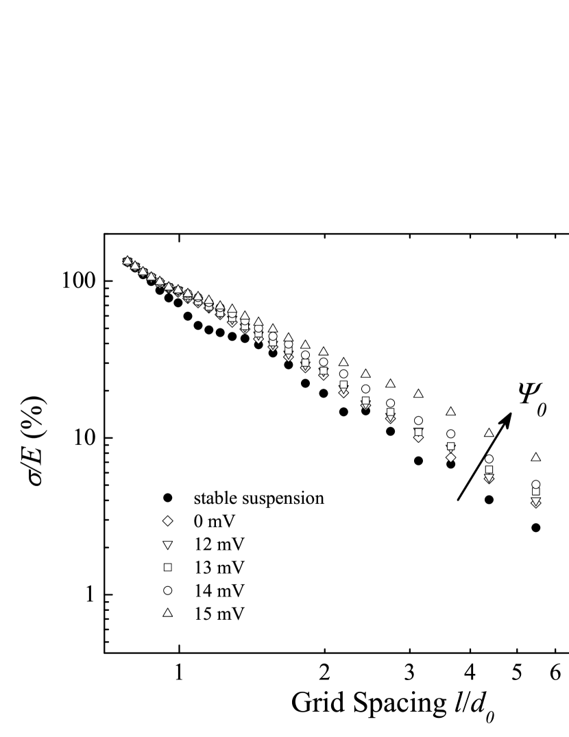
Figure 5: Relative density fluctuations for the various final microstructures and the stable suspension as a function of grid spacing.

In the following, two sets of comparisons are performed: Firstly, the various final microstructures are compared to the stable suspension. This comparison quantifies the length scale on which structural rearrangements take place during the coagulation. Secondly, the final microstructures with $\Psi_{0}>0$ mV are compared to the ”most homogeneous” microstructure with $\Psi_{0}$ = 0 mV. This set of comparisons reveals the length scale on which variations in heterogeneity are most pronounced.

The comparison of the various final microstructures to the initial, stabilized microstructure is shown in Fig. 6 in terms of $\Delta(n_{c})$ as given by Eq. (4) where superscripts $i$ and $j$ correspond to a final microstructure and to the initial microstructure, respectively. $\Delta(n_{c})$ is shown as function of the grid spacing $l$ normalized by the particle diameter $d_{0}=2r_{0}$.

All curves present an identical behavior, which essentially consists of three successive peaks with decreasing height towards a larger grid spacing. The location of the first, second and third peak is slightly above one, at two and at three particle diameters, respectively. The height of the individual peaks increases for increasing values $\Psi_{0}$.

More precisely speaking, the first peak is found at $1.09d_{0}$ for all final microstructures in comparison to the stable suspension. This grid spacing corresponds to a cell number of 8000 and therefore to the case where the average number of particles per cell is exactly one. This case is best reproduced for the stable suspension as for the final microstructures the standard deviation is roughly 20 to 27% larger. Physically, this peak is explained by the transition of the inter-particle potential from repulsive to attractive. Indeed, the repulsive potential in the case of the stable suspension causes all particles to occupy approximately the same volume as will be confirmed in Sec. III.3 by means of the Voronoi volume distribution. The switching of the inter-particle potential from repulsive to attractive causes the particles to form contacts resulting in an average particle separation of one particle diameter, which is smaller than the grid spacing of $1.09d_{0}$. This increases the probability of finding cells that are either empty or contain more than one particle and thus the standard deviation of the average number of particles per cell is increased.

The peaks at a grid spacing of approximately two and three particle diameters are considerably less pronounced than the peak at $1.09d_{0}$. In particular, the differences between the various final microstructures are larger than for the first peak. These differences will be elaborated in more detail in the following.

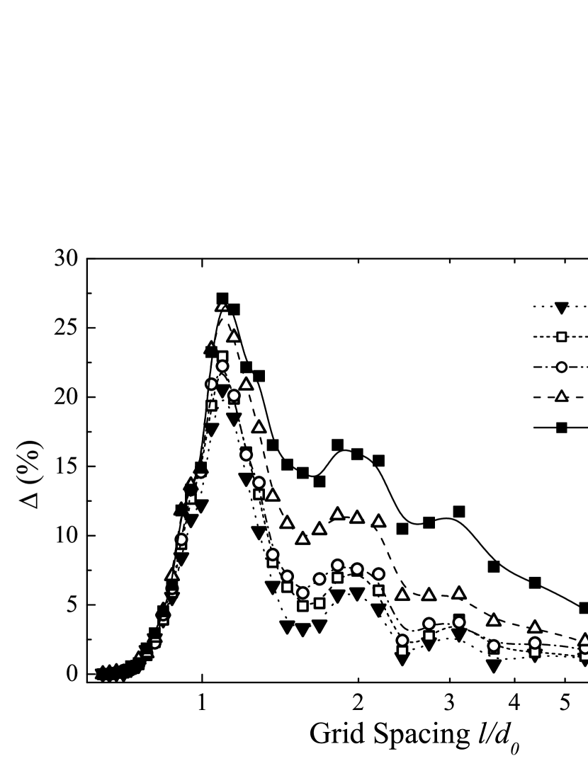
Figure 6: Relative difference between the density fluctuations of the various final microstructures and the stable suspension as a function of grid spacing. B-spline curves serve as guide to the eye.

The comparison between the final microstructures with $\Psi_{0}>0$ mV and the ”most homogeneous” microstructure with $\Psi_{0}$ = 0 mV is shown in Fig. 7. Here, superscripts $i$ and $j$ (Eq. (4)) correspond to one of the microstructures with $\Psi_{0}>$ 0 mV and to the microstructure with $\Psi_{0}$ = 0 mV, respectively. Over the whole range of grid spacings, the differences between the density fluctuations increase towards higher values of $\Psi_{0}$. This behavior correlates very well with the increase of porosity for increasing $\Psi_{0}$ as already observed in the previous section. Additionally, Fig. 7 reveals that the largest differences in terms or particle density between the ”most and least heterogeneous” microstructure ($\Psi_{0}$ = 15 mV and $\Psi_{0}$ = 0 mV, respectively) are found on a length scale between 1.3 and 2.2 particle diameters.

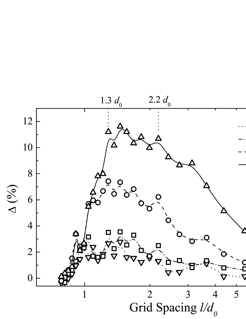
Figure 7: Relative difference between the density fluctuations of the various microstructures with ($\Psi_{0}>$ 0 mV) and the ”most homogeneous” microstructure ($\Psi_{0}$ = 0 mV) as a function of grid spacing. B-spline curves serve as guide to the eye.

III.3 Voronoi Volume Distribution

As stated in Sec. II.3 the distribution of Voronoi volumes $P(\nu)$ describes the deviation of a given structure from a perfectly crystalline packing, for which $P(\nu)$ is a delta function and all particles occupy the same volume. For random particle structures $P(\nu)$ broadens and as will be shown in the following, the width of the distribution can be interpreted as the heterogeneity of a structure.

We’ve calculated $P(\nu)$ for the stable suspension and the various final microstructures as a function of $\nu=\frac{V-V_{min}}{\bar{V}-V_{min}}$, the free volume normalized by the mean free volume (Fig. 8, symbols). The distribution found for the stable suspension is significantly narrower in comparison to the final microstructures. In the case of the final microstructures, $P(\nu)$ broadens with increasing value of $\Psi_{0}$ indicating that larger fluctuations in Voronoi volumes are found with increasing heterogeneity.

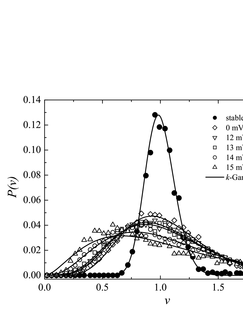
Figure 8: Voronoi volume distribution $P(\nu)$ for the various microstructures (symbols) and corresponding fits using the $k$-gamma distribution (lines).

The various microstructures were fitted using the $k$-Gamma distribution given in Eq. (5). The resulting curves are shown in Fig. 8 (lines) and the corresponding $k$- and R²-values are summarized in Table 3. $k$ decreases with increasing heterogeneity and can therefore be used as a measure for the DOH of the microstructures. The R²-values close to one indicate good fits. In particular, a very good fit quality was achieved for the stable and the final microstructures up to $\Psi_{0}$ = 14 mV. The R²-value for the $\Psi_{0}$ = 15 mV microstructure is lower. Indeed, Fig. 8 shows that for the $\Psi_{0}$ = 15 mV microstructure the agreement between the measured distribution and the fit curve for small Voronoi volumes is not as good as for the other curves. This might be related to the fact that during the generation of the $\Psi_{0}$ = 15 mV microstructure the energy barrier between primary and secondary minimum in the inter-particle potential was largest. This resulted in a few particle contacts still trapped in the secondary minimum (roughly 7% of the physical contacts). Particles trapped in the secondary minimum have an inter-particle distance of $2.16r_{0}$ instead of $2r_{0}$ upon complete coagulation, which may be a reason for the reduced fit quality towards smaller Voronoi volumes.

Table 3: $k$-Gamma fit results.

	$k$	R2
stable suspension	62.3	0.990
$\Psi_{0}$ = 0 mV	8.6	0.995
$\Psi_{0}$ = 12 mV	6.5	0.996
$\Psi_{0}$ = 13 mV	6.0	0.996
$\Psi_{0}$ = 14 mV	4.0	0.994
$\Psi_{0}$ = 15 mV	2.8	0.972

IV Summary and Conclusions

In this paper, we have analyzed three distinct microstructural characterization methods. Using these methods, scalar measures were introduced, which for the first time allow quantifying the DOH of particle packings.

• The exclusion probability gives an estimate of the pore size distribution by a random probing of the pore space. The ”more heterogeneous” microstructures present a considerably broader pore size distribution with a significantly longer tail than the distribution for the ”more homogeneous” microstructures. In particular, a continuous broadening is found with increasing heterogeneity. The cumulative exclusion probabilities were shown to follow error functions with parameter $a$ reflecting their width and thus measuring the structures’ DOH. Fit parameter $a$ increases with increasing heterogeneity.

• The density fluctuation method statistically analyzes the particle center density in dependence of the sampling length scale. The relative density fluctuation as function of the grid spacing presents a clear dependence on the heterogeneity of the microstructure: Over the whole range of grid spacings, the stable suspension exhibits the smallest density fluctuations. These fluctuations increase towards increasing values of $\Psi_{0}$ and thus increasing DOH, which is nicely reflected by increasing values of the integral measure $I_{df}$.

  An examination of the differences between the density fluctuations of two structures was found to be particularly useful as it allows determining the length scale on which the structures present the largest differences in heterogeneity. In the case of the ”most heterogeneous” microstructure the largest differences in comparison to the ”most homogeneous” one are found on a length scale between 1.3 and 2.2 particle diameters.

• The Voronoi volume distribution of the stable suspension is very narrow in comparison to the final microstructures, for which the distribution broadens with increasing heterogeneity. The various Voronoi volume curves were shown to follow $k$-gamma distributions. Parameter $k$, reflecting the width of the distribution and thus the structure’s DOH, decreases with increasing heterogeneity.

The behavior of the three parameters $a$, $k$ and $I_{df}$ is summarized in Fig. 9 showing $I_{df}$ (left scale) and $1/k$ (right scale) as a function of $a$. The solid lines suggest a pairwise affine dependence between $I_{df}$, $1/k$ and $a$. Thus, as far as the quantitative characterization of the DOH of the microstructures considered in this work is concerned, all methods, the pore size distribution, the density fluctuation method and the Voronoi volume distribution, can be considered as equivalent in the sense that the knowledge of one parameter permits to determine the others. However, parameter $k$ reflects changes in the DOH more sensitively than $a$ or $I_{df}$. Indeed, the normalization of $k$, $a$ and $I_{df}$ with respect to their maximum values reveals that parameter $k$ covers the interval $[0.04,1.0]$. This interval is significantly larger than the normalized ranges of $a$ and $I_{df}$, which are $[0.5,1.0]$ and $[0.86,1.0]$, respectively.

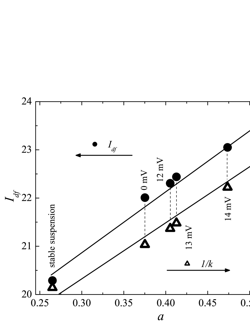
Figure 9: Interdependence between the measures of the degree of heterogeneity for the various microstructures: $I_{df}$ and $1/k$ as a function of $a$.

The interrelation between the three structural characterization methods can be understood as follows: The probability of placing a random point used for the determination of the pore size distribution into the free Voronoi volume of a particle is proportional to the particle’s free Voronoi volume. Thus, the broader the distribution of Voronoi volumes, the higher the probability of finding larger pores, which leads to a longer tail in the exclusion probability as shown in Fig. 3. The relation between the Voronoi volume distribution and the density fluctuation follows similar arguments: A broadening in the Voronoi volume distribution essentially means that there is a broader distribution in the nearest neighbor distances and therefore larger differences in the density fluctuations.

We have applied the methods to a set of monodispersed spherical particle packings representing stable and coagulated colloidal particle structures, but the methods could of course be generalized. The pore size distribution as determined by the Monte Carlo method employed in this work can be applied as it is to any porous media. In this sense, it is the most general method analyzed in this study. The fit using an error function however may not necessarily yield good results. In this case the integral measure $I_{ps}$ proposed in Sec. III.1 could be used or the width of the distribution could be determined empirically. The Voronoi volume distribution generally only requires that the elements constituting a structure are convex and in this case, the empirical distribution can be determined. To the authors’ knowledge a fit using the $k$-gamma distribution has however only been performed in the case of packings of monodispersed, spherical particles. As for the density fluctuation method, we have in this work considered the density of the particle centers. The method may be extended to a determination of the exact portion of the sphere volumes per cell, which however is computationally expensive. An alternative could be a cell-wise Monte Carlo integration of the partial sphere volumes, which would allow for a characterization of arbitrary porous structures using the density fluctuation method.

From an experimental point of view, the methods presented in this study rely on the possibility to determine the particle positions, which in the case of colloidal particles can be obtained using confocal laser microscopy for example Crocker and Grier (1996). In particular, the pore size distributions measured using mercury porosimetry Giesche (2006) and estimated using the exclusion probability are not equivalent since the latter overestimates the number of small pores due to the random probing of the pore space.

In this paper, we have introduced three scalar measures, which for the first time allow quantifying and comparing the heterogeneity of packings of spherical particles in terms of a DOH. These measures were calculated using distinct techniques and structural characterization methods. In view of these differences, the very nice correlation between the three DOH-measures is remarkable. Indeed, it suggests that the DOH is a microstructure’s inherent property and that any of the methods proposed in this work can be used to uniquely characterize and classify it. In terms of sensitivity however, considerable differences between the methods where found. Parameter $k$ reflects differences in the DOH most sensitively, followed by parameter $a$ and finally $I_{df}$. A further definition of an absolute DOH would require a suitable reference structure, which for example is either perfectly heterogeneous or perfectly homogeneous under the condition of being random.