The JCMT Legacy Survey of the Gould Belt: a first look at Orion B with HARP

Abstract

The Gould Belt Legacy Survey will survey nearby star-forming regions (within 500 pc), using HARP (Heterodyne Array Receiver Programme), SCUBA-2 (Submillimetre Common-User Bolometer Array 2) and POL-2 (Polarimeter 2) on the James Clerk Maxwell Telescope (JCMT). This paper describes the initial data obtained using HARP to observe ¹²CO, ¹³CO and C¹⁸O $J~{}=~{}3\rightarrow 2$ towards two regions in Orion B, NGC 2024 and NGC 2071. We describe the physical characteristics of the two clouds, calculating temperatures and opacities utilizing all three isotopologues. We find good agreement between temperatures calculated from CO and from dust emission in the dense, energetic regions. We determine the mass and energetics of the clouds, and of the high-velocity material seen in ¹²CO emission, and compare the relative energetics of the high- and low-velocity material in the two clouds. We present a CLUMPFIND analysis of the ¹³CO condensations. The slope of the condensation mass functions, at the high-mass ends, is similar to the slope of the initial mass function.

1 Introduction

1.1 The Gould Belt Legacy Survey

The Gould Belt Legacy Survey (GBS, Ward-Thompson et al., 2007) has been awarded 612 hours of time on the James Clerk Maxwell Telescope (JCMT) to survey nearby star-forming regions (within 500 pc), using HARP (Heterodyne Array Receiver Programme, Buckle et al., 2009), SCUBA-2 (Submillimetre Common-User Bolometer Array 2, Holland et al., 2006) and POL-2 (Polarimeter 2, Bastien, Jenness & Molnar, 2005). The HARP component will observe a large typical sample of prestellar and protostellar sources in three CO isotopologues. CO $J=3\rightarrow$2 and the same transition in ¹³CO and C¹⁸O are excited in the physical conditions of star-forming molecular clouds, where typical temperatures and densities are 10–50 K and 10⁴–10⁵ cm^-3. ¹²CO observations are used to search for and map any high-velocity outflows present, while the isotopologues measure the line widths and velocity profiles in the cores and filaments, resolving detailed kinematic and density properties of the cores. The GBS aims to provide a large and unbiased sample of star-forming material in the solar vicinity at relatively high spatial (8–14 arcsec) and spectral (0.05–1.0 ${\rm km\,s}^{-1}$) resolution. The GBS will trace the very earliest stages of star formation, through submillimetre continuum imaging using SCUBA-2 observations of low-temperature, high-column density regions, and provide an inventory of all the protostellar objects contained in the nearby molecular clouds of the Gould Belt, covering $\sim$ 700 deg². The HARP observations trace the kinematics of molecular gas in the cores and clusters at the same spatial resolution as the 850 $\mu$m SCUBA-2 observations of the dust emission. The key science goals of the HARP component of the GBS are (Ward-Thompson et al., 2007):

• To search for and map high-velocity outflows in the cores in order to differentiate between starless and protostellar cores.

• To derive simple constraints on the column density and CO depletion in these cores.

• To investigate support mechanisms and cloud/cluster/core evolution.

• To characterize the cloud kinematics in a wide variety of environments and investigate the role and evolution of turbulence in star formation.

The HARP targets for the GBS are a sample of the cloud regions that will be observed by SCUBA-2, with sizes $\sim$0.8 deg², and containing filaments and clustered star formation. This paper describes the initial HARP data obtained for two targets in Orion B, NGC 2024 and NGC 2071.

1.2 Orion B

The Orion B cloud complex is the closest region of high-mass star formation, lying at a distance of 415 pc (Anthony-Twarog, 1982; Menten et al., 2007). Five main star formation regions were identified from early wide field CO surveys: NCG 2024, NGC 2071, LBS 23 (HH 24), NGC 2068 and NGC 2023 (Tucker, Kutner & Thaddeus, 1973; Kutner et al., 1977; White & Phillips, 1981; Wilson et al., 2005). The cloud complex subtends an area of $\sim$ 26 deg², which corresponds to $\sim$ 1.5 kpc², and has a mass of $\sim$ 8 $\times$ 10⁴ M_⊙. The main star forming regions are clearly visible in the unbiased surveys for young stellar objects (Lada, Bally & Stark, 1991; Lis, Menten & Zylka, 1999; Motte et al., 2001; Mitchell et al., 2001; Johnstone, Matthews & Mitchell, 2006, hereafter J06) and in the dense gas tracer CS (Lada et al., 1991). Observations of individual sources in CO lines revealed a complex structure of outflows and gas motions (White, Phillips & Watt, 1981; Phillips, White & Ade, 1982), which are now known to be associated with extensive star formation activity (Flaherty & Muzerolle, 2008). A detailed summary of the Orion B regions can be found in the Handbook of Star Forming Regions (see chapters by Gibb, 2009; Bally, 2009; Meyer, 2009). The two GBS Orion B targets, NGC 2024 and NGC 2071, for which we have obtained the first data are shown as boxes in Fig. 1 overlaid on an extinction map of the Orion B cloud complex.

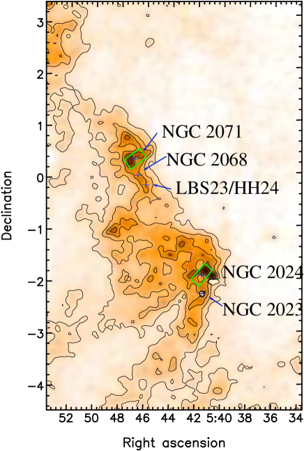
Figure 1: NGC 2024 and NGC 2071 shown within the Orion B cloud complex seen in visual extinction, A_ν from the atlas of Dobashi et al. (2005). The contours are drawn at A_ν=1,2,3,4,5,6 mag.

1.2.1 NGC 2024

NGC 2024 (The Flame Nebula, Anthony-Twarog, 1982) is a bright emission nebula that is crossed by a prominent dust lane. Intense radio continuum and recombination line emission (Krügel et al., 1982; Barnes et al., 1989; Bik et al., 2003; Rodríguez, Gómez & Reipurth, 2003), plus the detection of an infrared cluster, suggested the presence of ionizing star(s) of spectral type in the range O8 V-B2 V (Lada, Bally & Stark, 1991; Comerón, Rieke, & Rieke, 1996; Giannini et al., 2000; Haisch, Lada & Lada, 2000; Bik et al., 2003; Kandori et al., 2007).

Millimetre and submillimetre wavelength observations revealed a number of compact condensations that were believed to mark star forming sites. NGC 2024 has also been shown to contain a number of protostars positioned along a ridge of enhanced star formation activity, and its associated dense molecular material distributed as a filamentary structure (Mezger et al., 1988, 1992; Visser et al., 1998). Far-infrared and submillimetre polarimetric observations tracing the magnetic field structure of the star-forming ridge suggest it contains helical magnetic fields surrounding a curved filamentary cloud, possibly driven by the ionization front of the expanding Hii region (Hildebrand et al., 1995; Dotson et al., 2000; Greaves, Holland & Ward-Thompson, 2001; Matthews, Fiege, & Moriarty-Schieven, 2002). Previous molecular line observations of NGC 2024 have included studies of the outflow and thermal properties of the gas (Watt et al., 1979; White & Phillips, 1981; Phillips et al., 1988; Barnes et al., 1989; Richer et al., 1989; Barnes & Crutcher, 1990; Richer, Hills & Padman, 1992; Chernin, 1996; Mangum, Wootten & Barsony, 1999; Snell et al., 2000), revealing a complex and boisterous medium permeated with outflows, turbulence and complex gas dynamics.

1.2.2 NGC 2071

NGC 2071 is associated with a reflection nebula, molecular cloud and infrared cluster NGC 2071IR (White & Phillips, 1981; White et al., 1981; Persson et al., 1981; Motte et al., 2001; Johnstone et al., 2001, hereafter J01). The main infrared cluster has been resolved into eight distinct near-infrared sources having a total luminosity of 520 L_⊙ (Butner et al., 1990; Walther et al., 1993). The bipolar molecular outflow from NGC 2071 has been extensively studied in CO emission (White & Phillips, 1981; Snell et al., 1984; Scoville et al., 1986; Moriarty-Schieven, Hughes & Snell, 1989; Kitamura et al., 1990; Houde et al., 2001; Eislöffel, 2000), and is found to be amongst the most energetic bipolar outflows currently known, and extends for $\sim$ 2 pc (Margulis & Snell, 1989; Chernin & Masson, 1992; Chernin & Welch, 1995; Stojimirovic, Snell & Narayanan, 2008). This outflow is also seen in the shock excited 2.12 $\mu$m H₂ line (Persson et al., 1981; Lane & Bally, 1986; Burton, Geballe & Brand, 1989; Garden, Russell & Burton, 1990; Aspin, Sandell & Walther, 1992).

Snell & Bally (1986) have reported the presence of several extended radio continuum sources. Subsequent observations of H₂O masers and the associated radio continuum emission (Smith & Beck, 1994; Torrelles et al., 1998; Seth, Greenhill & Holder, 2002) suggest that the infrared sources IRS 1 and IRS 3 have strong winds, and are surrounded by rotating circumstellar disks. Further outflow activity around IRS 3 was suggested by its H₂ emission (Aspin et al., 1992) to indicate the presence of a circumstellar disk oriented perpendicular to the main outflow axis (Walther et al., 1993; Torrelles et al., 1998), that presumably contains a massive protostar.

1.2.3 Outline

In this paper, we present the initial heterodyne data on Orion B taken for the GBS. We determine characteristic physical properties for two clouds, NGC 2024 and NGC 2071, comparing and contrasting regions with varying physical characteristics. We present measurements of temperature and opacity across the regions, using these to provide temperature- and opacity-corrected masses and energetics of the clouds and the high-velocity material. We use our ¹³CO data to investigate clumpy structure within the clouds, calculate the mass function of the condensations, and compare the values found with core mass functions in these regions, and to the initial mass function. Sec. 2 provides an overview of the observations and data reduction. Sec. 3 describes the reduced data sets, highlighting regions of interest within the clouds with reference to previous observations. Sec. 4 presents the physical characteristics of opacity, temperature, energetics and kinematics for the clouds, while Sec. 5 presents an analysis of the condensations as traced by ¹³CO emission. We summarize the results presented in the paper in Sec. 6.

2 Observations

2.1 Overview of HARP

HARP is a recently-commissioned spectral-imaging receiver for the JCMT operating at submillimetre wavelengths (Buckle et al., 2009; Smith et al., 2003, 2008). It works in conjunction with the new back-end correlator, ACSIS (Auto-Correlation Spectral Imaging System, Buckle et al., 2009; Dent et al., 2000) offering high-spectral and spatial resolution, the latter matched to that of SCUBA-2 (Holland et al., 2006). HARP maps spectral lines in the 325-375 GHz atmospheric window, the JCMT B-band frequencies, where transitions of some of the most abundant molecules in the interstellar medium reside. The CO, ¹³CO and C¹⁸O $J=3\to 2$ lines in this window are used by the GBS to trace dense and/or warm gas around star-forming cores. The HARP imaging array consists of 16 SIS detectors arranged in a $4\times 4$ grid, separated by 30 arcsec. The beam size is 14 arcsec at 345 GHz, which means this array arrangement under-samples the focal plane with respect to Nyquist and further data points must be taken in between the nominal on-sky positions to produce a fully-sampled map. HARP works in single sideband mode, with typical receiver noise temperatures under 150 K and main-beam efficiencies of $\eta_{\mathrm{mb}}=0.61$ (Buckle et al., 2009). The K-mirror rotates the array with respect to the plane of the sky to maximize the observing efficiency, for instance allowing large raster scan maps to be made with the array oriented at an angle to the scan direction. ACSIS provides either wide-band (up to 1.9 GHz wide) or high-resolution spectra (up to 31 kHz channels). Additionally the IF can be separated into two sub-bands to allow simultaneous imaging of two close-together transitions e.g. the ¹³CO and C¹⁸O $J=3\to 2$ lines shown here.

2.2 Description of Observations

The observations presented here comprise 31.3 hrs of data taken on multiple nights from November 2007 to October 2008. The system temperatures, which are measured for each detector in every observation, varied (across different weather bands) from 344 to 684 K for the ¹²CO and 343 to 575 K for the ¹³CO/C¹⁸O data. Two fields in Orion B are analyzed: (i) NGC 2024, $(10.8\times 22.5)$ arcmin² centred on 05^h41^m39^s.8, -01${}^{\hbox{${}^{\circ}$}}$54${}^{\hbox{${}^{\prime}$}}$27${}^{\hbox{${}^{\prime\prime}$}}$ (J2000) at PA$=-40$ deg (east of north) (ii) NGC 2071, $(13.5\times 21.6)$ arcmin², centred on 05^h47^m00^s.0, +00${}^{\hbox{${}^{\circ}$}}$19${}^{\hbox{${}^{\prime}$}}$53${}^{\hbox{${}^{\prime\prime}$}}$ (J2000) angled at PA$=-55$ deg. The maps were taken in the raster position-switched observing mode, where spectra are taken “on-the-fly” with the telescope constantly scanning in a direction parallel to the sides of the map, taking spectra separated at 7.3 arcsec along this direction. The array is inclined at an angle of $\sim$14 deg to the scan direction which produces rows separated by 7.3 arcsec perpendicular to the scan direction automatically (Buckle et al., 2009). At the end of a scan row, the map is displaced half the array spacing perpendicular to the scan direction before a new row is started. This overlaps half of the new scan row’s data points with the first to double the integration time and even out any noise variations due to missing receptors or intrinsic differences in receptor performance. The noise is further evened-out by observing a second map scanning in a perpendicular direction to the first to “basket-weave” the field.

Separate absolute off positions were used for each field: (1) 05^h39^m00^s,-01${}^{\hbox{${}^{\circ}$}}$00${}^{\hbox{${}^{\prime}$}}$00${}^{\hbox{${}^{\prime\prime}$}}$ for NGC 2024 and (2) 05^h43^m44^s, +00${}^{\hbox{${}^{\circ}$}}$21${}^{\hbox{${}^{\prime}$}}$42${}^{\hbox{${}^{\prime\prime}$}}$.2 for NGC 2071. Each was verified to be absent of emission by examining short 60 s position-switched ‘stare’ observations towards each position in ¹²CO. A low-resolution ¹²CO mode (1 GHz bandwidth with 977 MHz channel spacing) was used for this inspection as it provided lower noise and ensured the other weaker isotopologues would also be free of emission.

2.2.1 The GBS HARP/ACSIS configuration

The ¹²CO data were taken in an ACSIS dual sub-band mode: (1) with modest resolution to map the broad line flows, at a rest frequency of 345.796 GHz, with the 1 GHz bandwidth divided into 1024 channels, separated by 977 kHz ($\sim$0.85 km s^-1) and (2), simultaneously, with higher resolution to map the detail of outflows close to the ambient cloud velocity, again at a rest frequency of 345.796 GHz, with 250 MHz bandwidth divided into 4096 channels, separated by 61 kHz ($\sim$0.05 km s^-1). Similarly, the ¹³CO/C¹⁸O data were taken in a high-resolution dual sub-band mode, each sub-band has a rest frequency of 330.588 or 329.331 GHz respectively with the 250 MHz band separated into 4096 61 kHz channels (at a spacing of 0.055 km s^-1).

2.3 Data Reduction

The data were reduced using the Starlink project software, with KAPPA (Currie et al., 2008) routines used to mask out poorly-performing detectors and calculate a self-flat (see Curtis, Richer & Buckle, 2009) for each observation. SMURF (Jenness et al., 2008) routines were used to make the cube using a Gaussian gridding technique, with 6 arcsec pixels and a 9 arcsec beam, giving an effective angular resolution of 16.6 arcsec in the final datacubes. KAPPA routines were then used to remove a linear baseline and crop the edges of the cubes spatially and spectrally. These data are presented as a ‘first look’ at the data being gathered for the GBS towards Orion. Data in the isotopically-substituted species towards these regions are still being collected, and the final data sets will have a much increased signal-to-noise. Table 1 describes the mean noise achieved in the datacubes collected to date, and the noise requirements of the final GBS data products. Data are presented in units of antenna temperature ($T_{A}^{*}$, Kutner & Ulich, 1981), which can be converted to main beam temperature ($T_{\rm mb}$) using $T_{\rm mb}$ = $T_{A}^{*}/\eta_{\rm mb}$.

Table 1: Current and required noise levels of GBS Orion B data

	current levelsa			required levelsb
Source	12CO	13CO	C18CO	12CO	13CO	C18CO
	mean 1$\sigma$ rms /K			mean 1$\sigma$ rms /K
NGC 2024	0.10	0.26	0.28	0.3	0.25	0.3
NGC 2071	0.11	0.32	0.43	0.3	0.25	0.3

^a6 arcsec pixels, 16.6 arcsec beam, 1.0 (¹²CO)/0.1(¹³CO/C¹⁸O) ${\rm km\,s}^{-1}$ channels.
^b7.5 arcsec pixels, 14 arcsec beam, 1.0 (¹²CO)/0.1(¹³CO/C¹⁸O) ${\rm km\,s}^{-1}$ channels.

3 Results

3.1 HARP spectral imaging

3.1.1 NGC 2024

Fig. 2 displays the total integrated intensity images across the full width of the emission lines towards NGC 2024 in ¹²CO 3$\to$2 (-20.0–50.0 ${\rm km\,s}^{-1}$), ¹³CO 3$\to$2 (4.0–16.0 ${\rm km\,s}^{-1}$) and C¹⁸O 3$\to$2 (6.0–14.0 ${\rm km\,s}^{-1}$). In this cloud, the integrated intensity image in ¹²CO is dominated by emission to the north of the map, particularly along a ridge extending south-west of the sources FIR1–7 (marked in Fig. 2 with white crosses). A cavity is seen to the north-west of this position, with the rest of the ¹²CO emission surrounding the cavity in a clumpy ring. The cavity marks a region of bright optical emission. Fig. 3 shows the digitized sky survey (DSS) infrared image overlaid with ¹²CO contours. The dense ridge where we see the brightest molecular emission appears as a dark dust lane in the optical image. The bright optical filaments appear in regions which lack ¹²CO emission. In particular, the large cavity contoured in ¹²CO integrated intensity emission clearly follows the shape of the bright optical emission. The peak of the ¹³CO emission is seen in the ridge containing the FIR sources. Further emission follows the ¹²CO emission, delineating a cavity surrounded by a ring of clumpy, filamentary structure. The C¹⁸O emission peaks on the positions of the FIR sources in the ridge. Weaker, fragmented and clumpy emission surrounds the cavity seen in ¹²CO and ¹³CO.

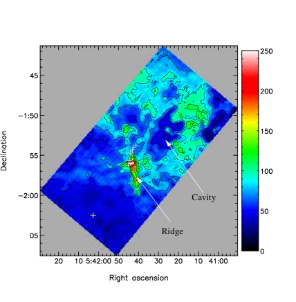
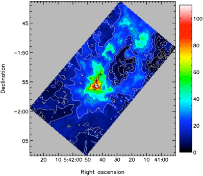
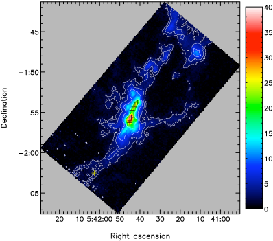
Figure 2: Integrated intensity images of ¹²CO (top), ¹³CO (middle) and C¹⁸O (bottom) towards NGC 2024. Crosses mark the positions of sources FIR1–7, and an isolated continuum source to the far south. Contours are ¹²CO: from 30 K ${\rm km\,s}^{-1}$ with 20 K ${\rm km\,s}^{-1}$ steps; ¹³CO and C¹⁸O: from 2 K ${\rm km\,s}^{-1}$, with contour levels doubling at every step.

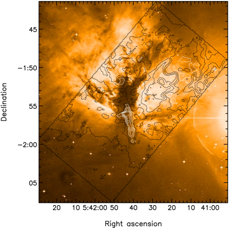
Figure 3: DSS infrared image of NGC 2024 overlaid with ¹²CO contours as in Fig. 2.

The ¹²CO spectra show evidence of several velocity components along the line of sight. Fig. 4 shows the spectra from a single pixel at the peak of C¹⁸O emission, from the three isotopologues. Also shown is a composite spectrum averaged over the observed region. The high-resolution ¹²CO spectrum shows four distinct peaks, at 4.6 ${\rm km\,s}^{-1}$, 8.3 ${\rm km\,s}^{-1}$, 11.2 ${\rm km\,s}^{-1}$and 13.0 ${\rm km\,s}^{-1}$. The ¹³CO spectrum has components at 4.2 ${\rm km\,s}^{-1}$, 8.7 ${\rm km\,s}^{-1}$ and 11.3 ${\rm km\,s}^{-1}$, while the C¹⁸O line has a main component at 11.0 ${\rm km\,s}^{-1}$, with a shoulder extension at 9.2 ${\rm km\,s}^{-1}$. These line profiles suggest self absorption in the ¹²CO line at 9.6 ${\rm km\,s}^{-1}$and 11.9 ${\rm km\,s}^{-1}$. Previous observations have also found several velocity components towards NGC 2024 (e.g. Emprechtinger et al., 2009). At 9 ${\rm km\,s}^{-1}$, the dense ridge, thought to be in the foreground, is seen as a separate component in C¹⁸O and ¹³CO, while there is a dip in the ¹²CO spectrum. This supports the suggestion that emission from the blue-side of the ¹²CO line is being absorbed by foreground material in the dense ridge (Emprechtinger et al., 2009; Graf et al., 1993). The main ¹³CO and C¹⁸O components peak near 11 ${\rm km\,s}^{-1}$, the velocity of the extended molecular cloud in the background (e.g. Barnes et al., 1989), and we also see a ¹²CO component at this velocity. The dip in the ¹²CO spectrum at 11.9 ${\rm km\,s}^{-1}$, which is part of the main component of the ¹³CO and C¹⁸O emission, suggests that there may be a further foreground component at this velocity which is absorbing the ¹²CO emission. The self-absorption of the ¹²CO emission undoubtedly causes its different peak position to the isotopologues tracing higher column density material. The multiple line-of-sight components are not clearly seen in spectra averaged over the whole region, and demonstrate the importance of high-spectral and spatial resolution observations in understanding the kinematics of star formation/molecular clouds, especially in clustered regions.

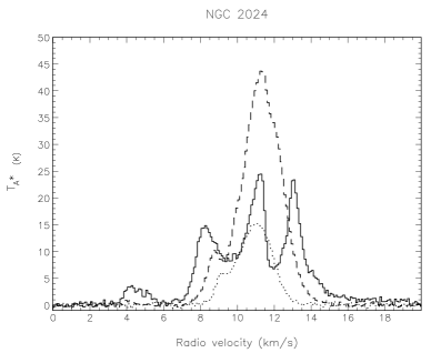
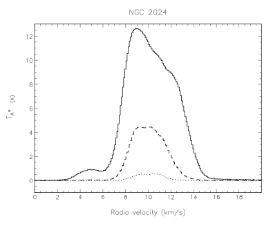
Figure 4: Spectra from a single pixel position (5^h41^m44^s.6 -1${}^{\hbox{${}^{\circ}$}}$55${}^{\hbox{${}^{\prime}$}}$33${}^{\hbox{${}^{\prime\prime}$}}$, top) and averaged over the whole cloud (bottom) of ¹²CO (solid line) ¹³CO (dashed line) and C¹⁸O (dotted line) towards the C¹⁸O peak in NGC 2024. All of the spectra have been observed at high-resolution, and binned to 0.1 ${\rm km\,s}^{-1}$.

Fig. 5 shows position-velocity (PV) diagrams of the three isotopologues across a large section of NGC 2024. The integrated intensity image in the left is marked with two lines showing the right ascension and declination cuts used. In the ¹²CO map, we can see a velocity gradient running north-south, from $\sim$13.0 ${\rm km\,s}^{-1}$ in the south to $\sim$10.0 ${\rm km\,s}^{-1}$ in the north. High-velocity material is seen as extended filaments across much of the PV diagrams, with the brightest high-velocity material seen associated with the ridge in the declination cut. The cavity previously described is labelled in the right ascension cut, at two velocity intervals straddling the main bulk of the molecular cloud at 11.0 ${\rm km\,s}^{-1}$. From 12.0–14.0 ${\rm km\,s}^{-1}$ the cavity shows a distinct velocity gradient along its edge, and is narrower than the outline seen at velocities 8.0–10.0 ${\rm km\,s}^{-1}$. The lower-velocity component of the cavity does not have the same velocity gradient along the edge. The very high-velocity outflow material is only clearly seen in the ¹²CO PV diagrams, but emission from ¹³CO shows extensions in velocity that suggest it is associated with outflow material. Both the ¹²CO and ¹³CO show compact clumps of emission at blue-shifted velocities near 4 ${\rm km\,s}^{-1}$, one of the components revealed in the spectra (Fig. 4). The ¹²CO PV diagrams show filaments extending between the clumps and the bulk of the emission, suggesting these clumps could be physically associated with the cloud, possibly through wind-driven activity. The emission at red-shifted velocities, from 12–14 ${\rm km\,s}^{-1}$, shows a much smoother distribution than the blue-shifted emission. The C¹⁸O emission is very compact in velocity, tracing the bulk of the dense material in the ridge, and no longer contains the component at 4 ${\rm km\,s}^{-1}$.

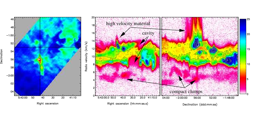
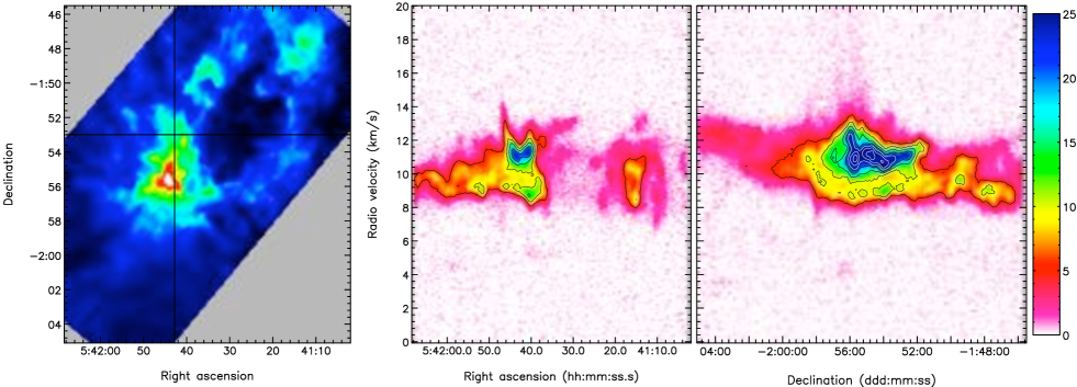
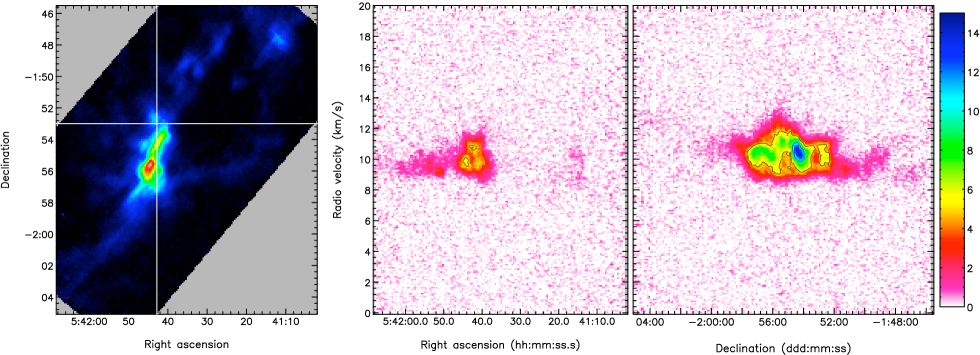
Figure 5: Position velocity maps of NGC 2024 in ¹²CO, ¹³CO and C¹⁸O, through the positions shown in horizontal and vertical lines in the integrated intensity image on the left.

3.1.2 NGC 2071

Fig. 6 shows total integrated intensity images across the full width of the emission lines for ¹²CO 3$\to$2 (-20.0–35.0 ${\rm km\,s}^{-1}$), ¹³CO 3$\to$2 (-3.0–18.0 ${\rm km\,s}^{-1}$) and C¹⁸O 3$\to$2 (5.0–12.0 ${\rm km\,s}^{-1}$) towards NGC 2071. The ¹²CO emission is dominated by a curved filament of emission, surrounding a compact, bright, optical emission region. Fig. 7 shows the DSS infrared image overlaid with ¹²CO contours towards NGC 2071, showing the ¹²CO emission nearly surrounding the bright nebula. The ¹³CO and C¹⁸O emission peaks along the compact ridge, but both show a different spatial structure to the ¹²CO emission at the southern end of the ridge, at the position of the optical nebula. In ¹³CO and C¹⁸O, the emission to the south, where the ¹²CO integrated intensity falls off, displays separate arcs.

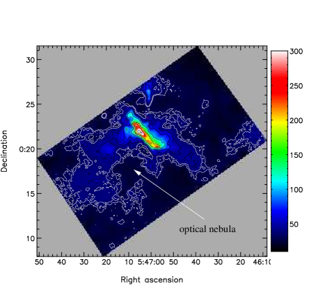
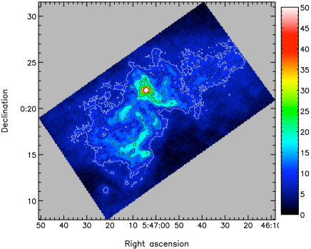
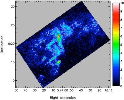
Figure 6: Integrated intensity images of ¹²CO (top), ¹³CO (middle) and C¹⁸O (bottom) towards NGC 2071. Contours are ¹²CO: 30,35 (white) and 45,65,105,185,345 (black) K ${\rm km\,s}^{-1}$; ¹³CO 7,9 (white) and 11,15,21,29,39 (black) K ${\rm km\,s}^{-1}$; C¹⁸O: 2 (white) and 4,7 (black) K ${\rm km\,s}^{-1}$. The first C¹⁸O contour is at 5$\sigma$.

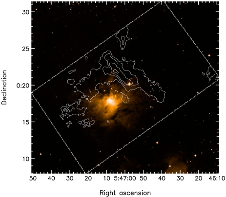
Figure 7: DSS infrared image of NGC 2071 overlaid with ¹²CO contours as in Fig. 6.

The spectra towards individual positions in NGC 2071 are shown in Fig. 8. At the systemic velocity of the cloud, around 10 ${\rm km\,s}^{-1}$, the ¹²CO is heavily self-absorbed, even in the low-density regions near the optical nebula (Fig. 8, top). Towards the peak of emission from C¹⁸O (Fig. 8, middle), emission from ¹³CO is also self-absorbed. The absorption dip in ¹²CO emission is also clear in the spectra averaged across the whole cloud (Fig. 8, bottom).

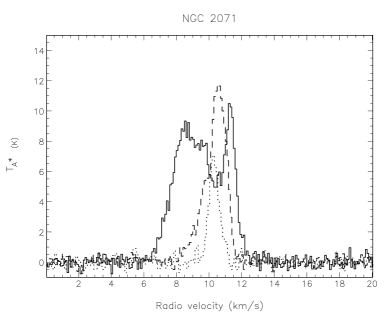
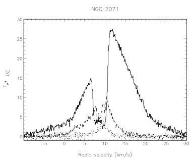
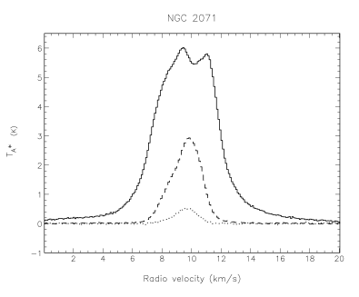
Figure 8: Spectra from single pixel positions; (top) 5^h47^m04^s.4 +0${}^{\hbox{${}^{\circ}$}}$14${}^{\hbox{${}^{\prime}$}}$53${}^{\hbox{${}^{\prime\prime}$}}$ towards the optical nebula; (middle) 5^h47^m04^s.0 +0${}^{\hbox{${}^{\circ}$}}$21${}^{\hbox{${}^{\prime}$}}$53${}^{\hbox{${}^{\prime\prime}$}}$, towards the C¹⁸O peak; and averaged over the whole cloud (bottom) of ¹²CO (solid line) ¹³CO (dashed line) and C¹⁸O (dotted line) in NGC 2071.

Fig. 9 shows the PV diagrams for NGC 2071, as for Fig. 5. We see high-velocity material from ¹²CO and ¹³CO, and evidence for the C¹⁸O emission tracing lower-velocity outflow material. There is no clear velocity gradient through the cloud. The ¹²CO and ¹³CO PV diagrams along a cut in right ascension suggest that there may be a second component along the line of sight to the west, or that the cloud is more extended in velocity in this region. In contrast to NGC 2024, towards NGC 2071, we do not see any clear features in the ¹²CO PV diagram that may be associated with cavities or bubbles carving out to the cloud edges through activity within the cloud. The C¹⁸O emission shows a compact, clumpy structure in the PV diagrams.

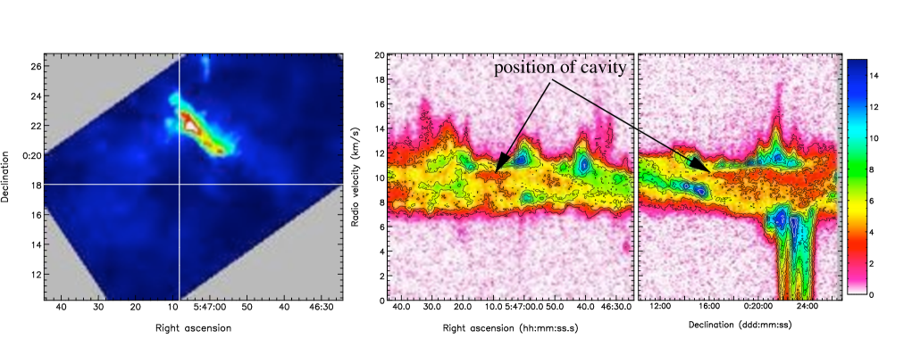
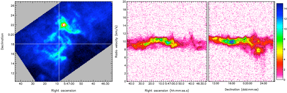
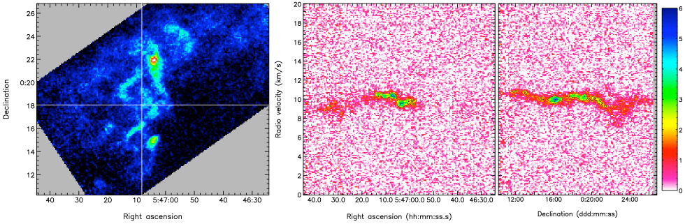
Figure 9: Position velocity maps of NGC 2071 in ¹²CO, ¹³CO and C¹⁸O, as for Fig. 5.

3.2 High-velocity material

Figs. 10 and 11 show false colour red, green and blue images of the average intensity across the ¹²CO line profile towards NGC 2024 and NGC 2071, where the emission near the systemic velocity of the clouds is shown in green, and the red- and blue-shifted gas is shown in the corresponding colour.

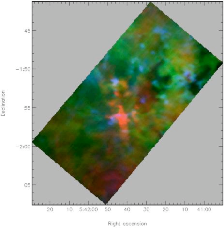
Figure 10: False colour image of the average ¹²CO emission towards NGC 2024 in red (13.2–19.2 ${\rm km\,s}^{-1}$), green (7.2–13.2 ${\rm km\,s}^{-1}$) and blue (1.2–7.2 ${\rm km\,s}^{-1}$) velocity channels.

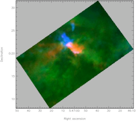
Figure 11: False colour image of the average ¹²CO emission towards NGC 2071 in red (13.1–19.1 ${\rm km\,s}^{-1}$), green (7.1–13.1 ${\rm km\,s}^{-1}$) and blue (1.1–7.1 ${\rm km\,s}^{-1}$) velocity channels.

Towards NGC 2024, a single region dominates the high-velocity red-shifted material, associated with an extended outflow from FIR5 and a compact outflow from FIR6 (Richer et al., 1989). Additionally, more diffuse components are seen throughout the map, which probably indicate different components along the line-of-sight, rather than protostellar outflows. However, there are two regions to the north, and several regions in the centre of the map where the relative position of red and blue emission, and the shape of the emission, suggest there are embedded outflow sources. The PV diagrams (Fig. 5) show several filamentary structures in velocity that may be associated with outflows that are less extensive in velocity than the obvious extremely high-velocity flows.

Fig. 12 shows contours of blue- and red-shifted emission overlaid on the integrated C¹⁸O intensity map for the main NGC 2024 outflow source. In the ¹²CO $J=3\rightarrow$2 emission, we see the high-velocity blue-shifted lobe is spatially compact, although extended in velocity. This is the only region in NGC 2024 where such high-velocity emission is detected.

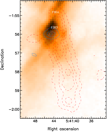
Figure 12: NGC 2024 high-velocity red- and blue-shifted ¹²CO emission. Red contours show emission from 14.5 to 40.0 ${\rm km\,s}^{-1}$, and blue contours show emission from -20.0 to 4.0 ${\rm km\,s}^{-1}$, both starting at 5 K ${\rm km\,s}^{-1}$, in steps of 20 K ${\rm km\,s}^{-1}$. The image shows the integrated C¹⁸O intensity. The suspected driving sources FIR5 and FIR6 have been labelled.

NGC 2071 is dominated by a high-velocity outflow, previously identified as one of the most energetic and collimated outflows ever discovered (e.g. Stojimirovic et al., 2008). The false colour image shows there are at least two more outflows, as suggested by Stojimirovic et al. (2008). The PV diagrams (Fig. 9) suggest how powerful this outflow is, with small extensions in velocity showing in the C¹⁸O emission. Again, the velocity-extended filamentary structures in this large-scale PV diagram suggest that there may be several protostellar outflows embedded within the cloud. In Sec. 4.5, we investigate the energy injection from outflows in these regions. Fig 13 shows the blue- and red-shifted contours overlaid on the C¹⁸O emission for the main NGC 2071 outflow region, overlaid with SCUBA sources (J06). Red- and blue-shifted outflow lobes can be identified, for at least three, and possibly five sources.

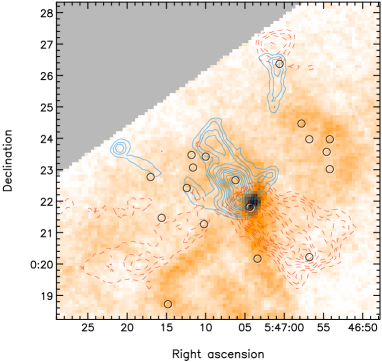
Figure 13: NGC 2071 high-velocity red- and blue-shifted ¹²CO emission. Red contours, show emission from 14.5 to 35.0 ${\rm km\,s}^{-1}$, blue contours show emission from -25.0 to 0.5 ${\rm km\,s}^{-1}$, contour levels at 5,10,15,25,45,65,85,105,125,145 K ${\rm km\,s}^{-1}$. The image shows the integrated C¹⁸O intensity. Black circles denote positions of SCUBA cores (J06).

3.3 Low density material

Towards both regions, a cavity is seen in emission from ¹²CO, associated with an optically-bright Hii region. However the behaviour of the less abundant isotopologues, and the velocity structure of these regions is different towards the two clouds.

Towards NGC 2024, emission from all of the CO isotopologues falls off in this region, as can be seen in the integrated intensity maps (Fig. 2). The cavity is coincident with the bright optical emission, and it may be that we are seeing the CO disassociated by an Hii region. Fig. 14 shows the SCUBA 850 $\mu$m continuum image (Di Francesco et al., 2008) overlaid with C¹⁸O integrated intensity contours. The C¹⁸O emission closely follows the structure seen in the dust, and the clumpiness of both the dust and the C¹⁸O emission suggest that cores are present in a region surrounding the cavity. We present an analysis of all the ¹³CO condensations in Sec. 5.

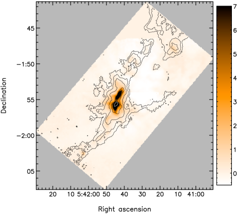
Figure 14: NGC 2024 SCUBA 850 $\mu$m maps (Di Francesco et al., 2008), overlaid with C¹⁸O integrated intensity contours. Contour levels are as Fig. 2.

In the NGC 2024 ¹²CO PV diagram (Fig. 5), the cavity can clearly be seen, and shows a different spatial structure at high and low velocities. There is an abrupt cut-off in emission across the lower velocities, from 8.0 to 10.0 ${\rm km\,s}^{-1}$. At the higher velocities, from 12.0 to 14.0 ${\rm km\,s}^{-1}$, there is a velocity gradient, and the eastern edge has a higher gradient in velocity than the western edge. If we are seeing an Hii region, then the different morphologies between the gas at low velocities and at high velocities may be giving information on the three-dimensional spatial structure. The low velocities, tracing material at the front of the cloud, have an abrupt cut-off to the emission because at this point, the material has broken out of the molecular cloud, and there is no more material entrained in the boundary layers. At higher velocities, if tracing material deeper into the cloud, the eastern edge is pushing into the dense molecular ridge seen in the C¹⁸O emission, while the western edge is pushing into more clumpy and fragmented material. This would account for the different velocity gradients seen in the PV diagrams, and supports the three-dimensional models suggested for this region (Emprechtinger et al., 2009; Barnes et al., 1989).

Fig. 15 shows the NGC 2071 SCUBA 850 $\mu$m map (Di Francesco et al., 2008), overlaid with C¹⁸O integrated intensity contours. The C¹⁸O emission does not follow the structure seen in the dust as closely as in NGC 2024, and it is in the region co-incident with the optical nebula that we see the most discrepancy. In the PV diagrams (Fig. 9), we see that the ¹³CO and C¹⁸O emission is clumpy and fragmented, both spatially, and in velocity, while the ¹²CO emission has a lower intensity region near the systemic cloud velocity, embedded within material at much higher velocities.

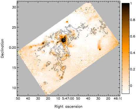
Figure 15: NGC 2071 SCUBA 850 $\mu$m map (Di Francesco et al., 2008), overlaid with C¹⁸O integrated intensity contours. Contour levels are as in Fig. 6.

4 Analysis of Cloud Parameters

4.1 Opacity

We calculate the gas opacity based on the line peak ratios of ¹²CO/¹³CO and ¹³CO/C¹⁸O. The intensity ratio is related to the opacity through:

$$R_{\rm 1318} = \frac{T_{\rm A}^{*}(^{13}{\rm CO})}{T_{\rm A}^{*}({\rm C^{18}O})}=\frac{1-\exp(-\tau_{13})}{1-\exp(-\tau_{18})}$$ (1)

$$R_{\rm 1213} = \frac{T_{\rm A}^{*}(^{12}{\rm CO})}{T_{\rm A}^{*}({\rm C^{13}O})}=\frac{1-\exp(-\tau_{12})}{1-\exp(-\tau_{13})}$$ (2)

This method makes several assumptions about emission from the isotopologues (see, for example Myers, Linke & Benson, 1983; Ladd, Fuller & Deane, 1998, for details). In particular that the beam efficiency, filling factor, and excitation temperature are the same for all the isotopologues, and that the ratio of line widths to the line of sight extent of the emitting gas is the same for all isotopologues.

Where the lines are optically thin, the ratio $R$ should tend to the abundance ratios, X[¹³CO/C¹⁸O]=8.4 and X[¹²CO/¹³CO]=70 for ¹³CO/C¹⁸O and ¹²CO/¹³CO respectively (Frerking, Langer & Wilson, 1982; Wilson, 1999). The ¹²CO/¹³CO intensity ratio maps for each source are shown in Fig. 16.

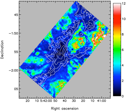
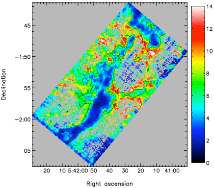
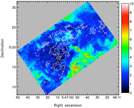
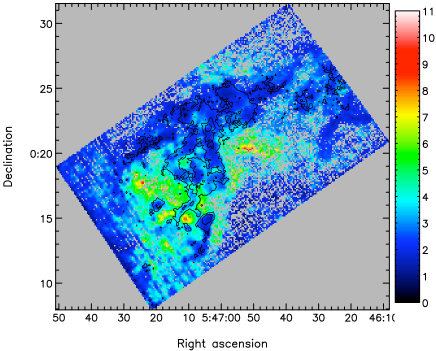
Figure 16: The ¹²CO/¹³CO (left) and ¹³CO/C¹⁸O (right) peak intensity ratios for regions with detections $<$3$\sigma$ towards NGC 2024 (top) and NGC 2071 (bottom), overlaid with C¹⁸O integrated intensity contours. The ¹³CO/C¹⁸O ratio data has been smoothed by a Gaussian with 12 arcsec FWHM to make the features more visible in these images.

From the ratio maps, we can estimate the abundance ratios from the values the ratios tend to towards the edge of detected emission regions, where we expect the lines to be optically thin. At the edges of the C¹⁸O emission regions, $R_{\rm 1318}$ tends to 8–12 in NGC 2024, and we therefore adopt X[¹³CO/C¹⁸O]=10 for NGC 2024. For NGC 2071, $R_{\rm 1318}$ tends to 6–9, so we similarly adopt X[¹³CO/C¹⁸O]=7.5. We detect ¹²CO and ¹³CO across the full extent of the mapped region, and the integrated intensity ratio does not approach the expected abundance ratio of $\sim$70. The highest ratios that we detect are $\sim$20, suggesting that ¹²CO is optically thick in the line core everywhere in both clouds, and so we use X[¹²CO/¹³CO]=70. Using the above equations and abundance ratios, mean opacities in the clouds are $\bar{\tau}$(¹²CO) $\sim$119, $\bar{\tau}$(¹³CO) $\sim$1.7, and $\bar{\tau}$(C¹⁸O) $\sim$0.17 in NGC 2024, while $\bar{\tau}$(¹²CO) $\sim$157, $\bar{\tau}$(¹³CO) $\sim$2.24, and $\bar{\tau}$(C¹⁸O) $\sim$0.3 in NGC 2071. These values suggest that C¹⁸O is generally optically thin, while ¹³CO is marginally optically thick, and ¹²CO is optically thick throughout both clouds. Note that self-absorption in the line profiles, which we see towards the densest regions, means that the opacity will be over-estimated for ¹²CO, and to a lesser extent for ¹³CO.

4.2 Temperature

Assuming local thermodynamic equilibrium (LTE), the excitation temperature ($T_{\rm ex}$) of the gas can be calculated from line peak temperature ($T_{\rm max}$) using the standard radiative transfer relation in an isothermal slab. Also assuming that the ¹²CO emission is optically thick ($\tau\rightarrow\infty$) and fills the beam in the line core across the cloud, then (e.g. Pineda, Caselli & Goodman, 2008):

$$T_{\rm ex}(3\rightarrow 2)=\frac{16.59{\rm K}}{{\rm ln}\left[1+16.59{\rm K}/\left(T_{\rm max}({\rm{}^{12}CO)}+0.036{\rm K}\right)\right]},$$ (3)

for regions where the ¹²CO line is not self-absorbed. We can identify the regions where there is self-absorption by comparison of the ¹²CO line profile with that of the ¹³CO line profile. Where the ¹²CO is optically thick and self-absorbed, the ¹³CO line peak temperature is higher than the ¹²CO line peak temperature. Towards these regions, ¹³CO is optically thick, and we use the equivalent form of Eq. 3 to calculate $T_{\rm ex}$ from ¹³CO. Fig. 17 shows $T_{\rm ex}$ across NGC 2024 (top) and NGC 2071 (bottom), calculated using both ¹²CO and ¹³CO.

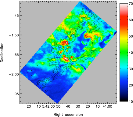
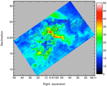
Figure 17: Excitation temperature (in K) for NGC 2024 (top) and NGC 2071 (bottom). To indicate regions where the ¹²CO may be self-absorbed, and so underestimating the excitation temperature, the contours show C¹⁸O integrated intensity.

NGC 2024 generally reaches higher excitation temperatures than NGC 2071. Towards NGC 2024, the mean excitation temperature is 31.8 K, which increases to $\ga$50 K in the dense regions, and $\sim$70 K in regions which are known to contain energetic outflows. Towards NGC 2071, the mean excitation temperature is 19.6 K, which increases to $\ga$30 K in the dense regions, and $\sim$50 K in the regions associated with energetic outflows.

Towards the dense cores of Orion B, kinetic temperatures have been published using line ratios of H₂CO, a molecule known to trace gas kinetic temperatures extremely well (Mangum & Wootten, 1993; Tothill & Mitchell, 2001; Mangum et al., 1999). Although only a few of these sources overlap with the regions we have observed, the excitation temperatures calculated from CO agree well with those calculated from H₂CO, except towards NGC 2024 FIR5, the probable driving source of the energetic outflow seen as a large red-shifted outflow lobe (Fig. 12). Average values for the small number of H₂CO dense cores, with the exception of NGC 2024 FIR5, are 44 K from H₂CO, and 39 K from CO. Given that the H₂CO transitions have a critical density of $\geq$3.9$\times$10⁶ cm^-3, while the critical density of the ¹²CO transition is $\sim$3.5$\times$10⁴ cm^-3, and that the velocity structure of these regions is relatively complex, this is surprising, and suggests the combination of ¹²CO and ¹³CO is a relatively good tracer of excitation conditions in dense regions. We have also compared our CO excitation temperatures with those derived from dust temperatures towards SCUBA cores in both clouds by J01, J06. Fig. 18 shows the integrated intensity maps of ¹²CO, overlaid with contours of C¹⁸O, and marked with the positions of the SCUBA dust cores from J01, J06. The cores are marked in green if $T_{\rm ex}(^{12}$CO)/$T_{\rm dust}$ $\leq$1.5, and in red if the ratio is $>$1.5. For the small number of cores that also have H₂CO measurements, the average dust temperature is 41 K, similar to the H₂CO and CO values. Towards NGC 2071, all of the SCUBA cores have CO and dust temperatures ratios $\leq$1.5, while towards NGC 2024, the ratio is $\leq$1.5 only towards the high column density regions of NGC 2024, along the molecular ridge. Towards NGC 2024, the cores where dust temperatures are similar to temperatures derived from CO are spatially grouped towards the highest column density regions. In NGC 2024, the differences in $T_{\rm ex}(^{12}$CO) and $T_{\rm dust}$ towards the lower column density regions may be evidence of sub-thermal excitation of CO. Given the complex velocity structure of these regions, and the complications that opacity adds to the line profile, observations utilizing all CO isotopologues so that opacity corrections can be made appear to be relatively good tracers of the gas and dust temperatures in energetic, densely clustered regions.

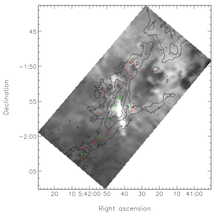
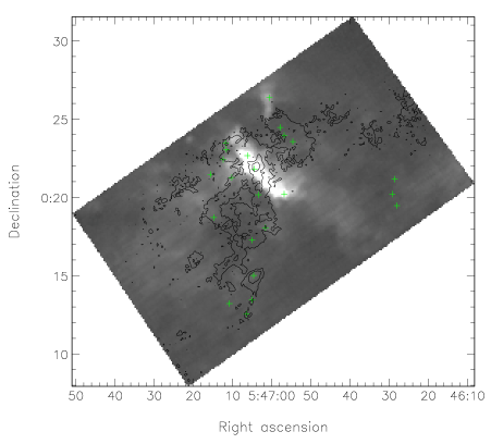
Figure 18: ¹²CO integrated intensity maps for NGC 2024 (top) and NGC 2071 (bottom), overlaid with C¹⁸O contours. SCUBA cores from J01, J06 are marked in green where the ratio $T_{\rm ex}$(¹²CO)/$T_{\rm dust}$ $\leq$1.5 and in red otherwise.

4.3 Mass and energetics

Since we have isotopic data, we can calculate the mass in the large-scale cloud, using the ¹²CO and ¹³CO data, which we detect everywhere. In the dense molecular ridge, where ¹²CO and ¹³CO line profiles are affected by self-absorption, we can use the C¹⁸O data, assuming LTE conditions. We compute the masses assuming $T_{\rm ex}$ is the same for all three isotopologues, and equal to the mean ¹²CO excitation temperature (Sec. 4.2). We correct for optical depth effects in the ¹²CO and ¹³CO data using the mean opacities $\bar{\tau}(^{13}\rm CO)$, and $\bar{\tau}(^{12}\rm CO)$ (Sec. 4.1). Following Garden et al. (1991) :

$$\rm N(C^{18}O) = 8.26\times 10^{13}\exp\left(\frac{15.81}{T_{\rm ex}}\right)$$ (4)

$$\times \frac{T_{\rm ex}+0.88}{1-\exp(\frac{-15.81}{T_{\rm ex}})}\int\tau{\rm\,dv}~{}{\rm cm^{-2}}$$

$$\rm N(^{13}CO) = 8.28\times 10^{13}\exp\left(\frac{15.87}{T_{\rm ex}}\right)$$ (5)

$$\times \frac{T_{\rm ex}+0.88}{1-\exp(\frac{-15.87}{T_{\rm ex}})}\int\tau{\rm\,dv}~{}{\rm cm^{-2}}$$

$$\rm N(^{12}CO) = 7.96\times 10^{13}\exp\left(\frac{16.6}{T_{\rm ex}}\right)$$ (6)

$$\times \frac{T_{\rm ex}+0.92}{1-\exp(\frac{-16.6}{T_{\rm ex}})}\int\tau{\rm\,dv}~{}{\rm cm^{-2}}$$

where we use the approximations:

$$\int\tau{\rm\,dv} = \frac{1}{\left[J(T_{\rm ex})-J(T_{\rm BG})\right]}\frac{\bar{\tau}}{1-e^{-\bar{\tau}}}\int T_{\rm mb}{\rm\,dv}~{}({\rm for}~{}\tau\geq 1)$$ (7)

$$\int\tau{\rm\,dv} = \frac{1}{\left[J(T_{\rm ex})-J(T_{\rm BG})\right]}\int T_{\rm mb}{\rm\,dv}~{}({\rm for}~{}\tau\ll 1)$$ (8)

$$J(T) = \frac{T_{0}}{\exp\left(\frac{T_{0}}{T}\right)-1}$$ (9)

$$T_{o} = \frac{h\nu}{k}$$ (10)

with $T_{\rm BG}$ = 2.7K. The mass is given by:

$$M_{\rm gas}=1.13\times 10^{-4}\mu_{H_{2}}m_{H}d^{2}\Delta\alpha\Delta\beta{\rm X}N({\rm CO})~{}~{}\hbox{M${}_{\odot}$}$$ (11)

where $\Delta\alpha\Delta\beta$ is the pixel area in arcsec², $d$ is the distance in pc, v is in ${\rm km\,s}^{-1}$and X is the isotopic abundance ratio of CO and its isotopologues relative to H₂. We adopt a mean molecular weight per H₂ molecule of $\mu_{H_{2}}$ = 2.72 to include helium, and X[¹²CO]=1.0$\times$10^-4, X[¹³CO]=1.4$\times$10^-6, X[C¹⁸O]=1.7$\times$10^-7 (Frerking et al., 1982; Wilson, 1999). The results are listed in Tab. 2. The masses that we find for optically thick ¹²CO are smaller than previous mapping observations of a 19 deg² region in Orion B, using a lower excitation transition, where a total mass of 8.3$\times 10^{4}$ M_⊙ was measured (Maddalena et al., 1986). The total mass we derive for NGC 2024 and NGC 2071, covering a region $\sim$100 times smaller in area and using optically thick ¹²CO, is 8.5$\times 10^{3}$ M_⊙. In ¹³CO, we find a total mass of 2.5$\times 10^{3}$ M_⊙. The total mass of gas that we detect in C¹⁸O towards both clouds is 1000 M_⊙. Emission from the optically thin isotopologue C¹⁸O traces a smaller region within the cloud, and does not suffer from the same uncertainties due to optical depth corrections. If the opacity corrections using mean values were accurate, we would perhaps expect the masses calculated from ¹²CO and ¹³CO emission to be similar to that calculated from C¹⁸O emission. However, the differences may be due to physical conditions within the clouds affecting the transitions differently. Towards NGC 2024 in particular, the many velocity components seen in the spectra indicate that a single excitation temperature and density along the line of sight may not be a good approximation of the conditions. The clouds may not be in LTE, and emission from the isotopologues subthermally excited. As suggested by Pineda et al. (2008), the shielding of material within the cloud leads to physical and chemical properties which can affect ¹²CO and ¹³CO differently to the rarer isotopologue C¹⁸O. We find a total mass of 1111 M_⊙ using ¹³CO data, if we assume that ¹³CO emission is also optically thin. The total mass calculated from ¹²CO under the assumption of optically thin emission is 65 M_⊙, indicating that emission from this isotopologue is, as calculated above, very optically thick, and tracing only the surface regions of the clouds. NGC 2024 contains more mass than NGC 2071, measured in all of the isotopologues.

The gravitational potential energy, $W$, of the cloud can be calculated assuming a density distribution $\rho~{}\propto r^{a}$ (MacLaren, Richardson & Wolfendale, 1988; Williams, de Geus & Blitz, 1994; Bertoldi & McKee, 1992). The kinetic energy, $E_{\rm kin}$, can be calculated by estimating the three-dimensional velocity dispersion, $\sigma_{v,3D}^{2}$, from the one-dimensional velocity dispersion of the average spectrum, $\sigma_{{}^{12}{\rm CO}}$, $\sigma_{{}^{13}{\rm CO}}$ or $\sigma_{\rm C^{18}{\rm O}}$:

$$W = -\frac{3}{5}\gamma\frac{GM_{\rm gas}^{2}}{R}$$ (12)

$$\gamma = \frac{1+a/3}{1+2a/5}$$ (13)

$$E_{\rm kin} = \frac{1}{2}M_{\rm gas}v^{2}$$ (14)

$$v^{2} = \sigma_{v,3D}^{2}=3\left[\sigma_{{\rm CO}}^{2}+\frac{kT}{m_{H}}\left(\frac{1}{\mu}-\frac{1}{m_{\rm CO}}\right)\right]$$ (15)

where $G$ is the gravitational constant, $k$ is Boltzmann’s constant, $T$ is the kinetic temperature of the gas, which we have taken to be equal to the mean ¹²CO excitation temperature and $m_{{\rm CO}}$ is the atomic mass of ¹²CO, ¹³CO, or C¹⁸O. We assume the clouds follow $\rho\propto r^{-2}$ density distributions, yielding $\gamma=5/3$. The LTE masses, kinetic and gravitational potential energies of both clouds are listed in Tab. 2.

Table 2: Table of masses and energetics

Cloud	LTE mass ($\times 10^{3}$ /M⊙)			$E_{\rm kin}$ ($\times 10^{40}$ /J)			$-W$ ($\times 10^{40}$ /J)
	12CO	13CO	C18O	12CO	13CO	C18O	12CO	13CO	C18O
NGC 2024	4.8	1.6	0.6	37.5	5.9	1.6	9.5	1.1	0.2
NGC 2071	3.7	0.9	0.4	24.5	1.6	0.4	5.7	0.3	0.1

NGC 2024, as well as containing more mass than NGC 2071, has greater kinetic and gravitational potential energies. The gravitational potential energy calculated from ¹²CO and ¹³CO is larger than the kinetic energy in both regions, implying that these clouds are both gravitationally bound. The emission from C¹⁸O, tracing much smaller regions containing all of the currently active outflows, has more kinetic energy. The line profiles and PV diagrams of ¹²CO and ¹³CO indicate that both of these isotopologues are tracing some of the high-velocity, presumably outflowing, material. In Sec. 4.5, we compare these values to the energetics in the high-velocity material.

4.4 Cloud kinematics

Fig. 19 shows the velocity at the line peak of the optically-thin gas. This has been created from the ¹³CO and C¹⁸O data, using ¹³CO in regions where the C¹⁸O line peak falls below the 3$\sigma$ level. Towards NGC 2024, a velocity gradient runs across the image, from 8 ${\rm km\,s}^{-1}$ in the north, to 10 ${\rm km\,s}^{-1}$ in the south, with the molecular ridge in the south seen in emission at 11.5 ${\rm km\,s}^{-1}$. The dust cavity is seen in material at $\ga$11.5 ${\rm km\,s}^{-1}$, surrounded by material at 8.0–10.0 ${\rm km\,s}^{-1}$, with a further higher velocity band to the northwest. In the southernmost part of the map, a band of high-velocity material appears, which is the tip of the NGC 2023 region. The velocity gradient can also be clearly seen in the ¹²CO PV diagram (Fig. 5). Towards NGC 2071, there is no obvious underlying velocity gradient. All of the velocity variations seen in the NGC 2071 map appear to be associated with current star forming activity in the cloud. In the south, there is a large region that is clearly red-shifted with respect to the rest of the cloud, which is in the same direction as the very energetic red-shifted outflow lobes seen towards NGC 2071 (Fig. 13)

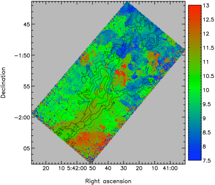
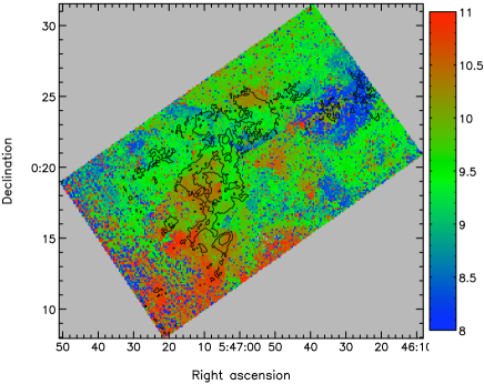
Figure 19: NGC 2024 map of the velocity at the line peak (in ${\rm km\,s}^{-1}$) for C¹⁸O where emission is above the 3$\sigma$ level, and ¹³CO at all other regions (top). ¹³CO is detected above the 3$\sigma$ level at all points in the map. The same Fig. for NGC 2071 (bottom).

Fig. 20 shows the equivalent width ($\int Tdv/T_{peak}$) for the optically thin emission towards the two regions. The exterior edges of the molecular ridge towards NGC 2024, traced by the outer contours of C¹⁸O, have lower velocity dispersions than the material within which it is embedded, and the energetic region near the FIR sources. Towards NGC 2071, the material with a lower velocity dispersion is perpendicular to the outflow direction. In the regions extending along the outflow, a cone-shape of higher velocity dispersion material can be seen.

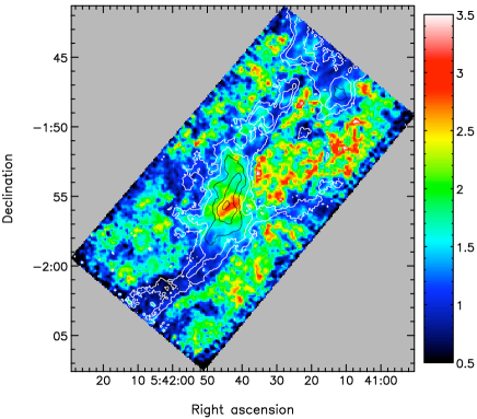
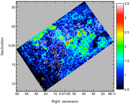
Figure 20: NGC 2024 map of equivalent width (in ${\rm km\,s}^{-1}$) for C¹⁸O where emission is above the 3$\sigma$ level, and ¹³CO at all other regions (top). ¹³CO is detected above the 3$\sigma$ level at all points in the map. The same Fig. for NGC 2071 (bottom). Data has been smoothed by a Gaussian with 12 arcsec FWHM to make the features more visible in these images.

4.5 Mass and energetics of the high-velocity material

Using the line centre of the average C¹⁸O spectrum to identify the velocity of the cloud, we calculate the total mass in the high-velocity material generated from the outflows using ¹²CO emission, with red- and blue-velocity extents across the line profile. We assume that the high-velocity emission is optically thin, and at a similar excitation temperature to the bulk of the gas, given by the mean ¹²CO excitation temperature, following the method in Sec. 4.3. We obtain masses of a few $\times$ 1 M_⊙. This is much lower than found using lower excitation transitions of ¹²CO and ¹³CO (e.g. Snell et al., 1984; Stojimirovic et al., 2008, although these authors used a combination of isotopologues across the velocity range for their calculation). For ¹³CO, where the assumption that the emission is optically thin in the line wings is more likely to be correct, we obtain masses $\sim$ a few $\times$ 10 M_⊙, in better agreement with those previously found, which suggests the optically thin assumption for ¹²CO line wings produced in outflows is not valid.

From the ¹³CO emission, we calculate the energy and momentum of this high velocity material using :

$$P = MV_{\rm char}$$ (16)

$$E_{k} = \frac{1}{2}MV_{\rm char}^{2}$$ (17)

where $V_{\rm char}$ is a characteristic velocity estimated as the difference between the maximum velocity with detectable emission in ¹²CO emission and the cloud velocity identified from the line centre velocity of a Gaussian fit to the average C¹⁸O line profile. For this reason, and since we do not account for the inclination to the line of sight for any outflows, the calculated values are upper limits. The mass, momentum and energy values for the red- and blue-shifted emission for both clouds are listed in Tab. 3.

Table 3: Mass and energetics of high-velocity material

Cloud	Velocity	Vchar	12CO Mass	13CO Mass	Energy	Momentum
		${\rm km\,s}^{-1}$	M⊙	M⊙	$\times 10^{40}$J	M⊙ ${\rm km\,s}^{-1}$
NGC 2024	red	32.3	4.50	19.64	2.03	634
NGC 2024	blue	25.2	3.38	14.59	0.92	367
NGC 2071	red	43.0	6.75	37.34	6.86	1604
NGC 2071	blue	39.2	5.66	28.01	4.29	1099

The total energy of the high-velocity material within the cloud is 100 times more than that calculated by investigating individual flows. Towards NGC 2071, Stojimirovic et al. (2008) found a total energy in the red and blue outflow lobes of 9.67$\times 10^{45}$ ergs, compared to our value of 11.15$\times 10^{47}$ ergs. The values we calculate are likely to be over-estimated, since we have used a maximum estimate for the characteristic velocity. Comparing these values to the kinetic energy of the cloud as measured from ¹³CO emission, the high-velocity material accounts for very little of the total kinetic energy in NGC 2024, while the high-velocity material dominates the kinetic energy in NGC 2071.

5 Analysis of the gaseous condensations

The structure of molecular clouds has been characterized in numerous ways in the literature, including identifying discrete objects in the emission (often termed clumps). By studying the properties of such clumps we hope to explore the properties of the cores, harboured by some of the clumps, which will go on to form stars. Frequently, automated clump-finding routines have been used, to look for clumps in an unbiased manner, in both spectral-line and dust continuum datasets. In this section, we undertake a statistical decomposition of the structure of the ¹³CO $J=3\to 2$ emission using the clumpfind algorithm (Williams et al., 1994), implemented in Starlink’s new CUPID package (Berry et al., 2007). The optically-thin C¹⁸O $J=3\to 2$ data will be a better tracer of the mass in the star-forming cores, where the ¹³CO line is saturated. Here we explore the ¹³CO $J=3\to 2$ bulk cloud emission. Many different terminologies have been used to name clumps in molecular clouds, here we call any individual object identified using clumpfind a ‘condensation’, to emphasize that it may not collapse to form a star.

The data were smoothed to 0.25 ${\rm km\,s}^{-1}$ spectrally to improve the signal to noise ratio but still maintain sufficient resolution to identify condensations with the narrowest anticipated line widths. At our assumed cloud temperatures (50 and 30 K for NGC 2024 and NGC 2071 respectively) the ¹³CO line widths expected from thermal broadening alone ($\sqrt{kT/m_{H}m_{CO}})$ are 0.4 ${\rm km\,s}^{-1}$ for NGC 2024 and 0.3 ${\rm km\,s}^{-1}$ for NGC 2071. At this resolution, the mean RMS noise across the map is reduced to 0.14 and 0.20 K for NGC 2024 and NGC 2071 respectively. We ran clumpfind using a level spacing of $2\sigma_{\rm RMS}$ (the value recommended by Williams et al. (1994) to reduce the contamination by noise) and a lowest level of $2\sigma_{\rm RMS}$, which ensures the minimum peak intensity of a condensation is $4\sigma_{\rm RMS}$. Additionally, condensations were rejected if they touched any edge of the data array, contained fewer than 16 (3D) pixels or were smaller than the beam size. These parameters resulted in a catalogue of 1561 and 1399 condensations in NGC 2024 and NGC 2071 respectively.

Previous studies of the clump distribution in the dust continuum emission of Orion B have identified a factor of $\sim 10$ fewer condensations than we do from the ¹³CO emission (J01, J06). This is probably because the SCUBA observations are not sensitive to flux on large-scales whereas the ¹³CO gas should trace this more ambient emission, which can account for the ¹³CO condensations identified which are not spatially associated with a dust clump. Additionally, the spectral information in the ¹³CO data may break up multiple condensations at distinct velocities along the line of sight, which may be superposed in continuum data. For each dust clump identified by J01 and J06 in our observing fields, we found the mean number of ¹³CO condensations whose peak lies within the radii of the dust clumps to be $\sim 7.4$ for NGC 2024 and $\sim 3.7$ for NGC 2071.

5.1 Condensation properties

In the catalogue generated by CUPID, the ‘size’ of each condensation along each axis (right ascension, declination, velocity) is given by the standard deviation of the pixel co-ordinate values about the centroid position, weighted by the pixel values, then corrected to remove the effect of instrumental smoothing. We define the radius of a condensation as the geometric mean of the size along axes 1 and 2 ($R_{1}$ and $R_{2}$):

$$R=\sqrt{R_{1}R_{2}}\mathrm{,}$$ (18)

where $R_{1}$ and $R_{2}$ have been already been deconvolved with the beam size.

For NGC 2024 the condensation radii range from $1.3\times 10^{-3}$ pc to 0.053 pc with a mean value of $0.018\pm 0.009$ pc. For NGC 2071 the values are similar; the radii range from $1.3\times 10^{-3}$ pc to 0.075 pc with a mean value of $0.017\pm 0.008$ pc.

We estimate the three-dimensional velocity dispersion of each condensation from the one-dimensional ¹³CO velocity dispersion, $\sigma_{{}^{13}{\rm CO}}$ (the size along axis 3 calculated by CUPID), as described in Sec. 4.3. For NGC 2024, the velocity dispersions range from 0.66 to 2.0 ${\rm km\,s}^{-1}$, with a mean value of $0.99\pm$0.23 ${\rm km\,s}^{-1}$. Again the values are similar for NGC 2071, ranging from 0.50 to 2.5 ${\rm km\,s}^{-1}$ with a mean of $0.88\pm$0.19${\rm km\,s}^{-1}$.

Assuming the clouds are in LTE and the ¹³CO $J=3\to 2$ transition is optically thin, the masses of the ¹³CO clumps can be derived following Sec. 4.3. At moderately high densities (which we expect the ¹³CO $J=3\to 2$ transition to probe, given its critical density) the cloud gas and dust should be coupled and at the same temperature (Burke & Hollenbach, 1983). The mean temperatures of the dust clumps associated with our ¹³CO condensations, computed by J06 and J01, are $45\pm 11$ K and $26\pm 8$ K for NGC 2024 and NGC 2071 respectively. We therefore adopt excitations temperatures of $T_{\rm ex}=50$ and 30 K for NGC 2024 and NGC 2071 respectively in our mass calculations, which are also consistent with the temperatures we derived in Sec. 4.2 (see Fig. 17).

In NGC 2024, we find the masses of the condensations range from $2.6\times 10^{-3}~{}\hbox{M${}_{\odot}$}$ to $13~{}\hbox{M${}_{\odot}$}$, with a mean value of $0.52\pm 1.2~{}\hbox{M${}_{\odot}$}$. For NGC 2071 the condensations are less massive, ranging from $3.4\times 10^{-3}~{}\hbox{M${}_{\odot}$}$ to $5.3~{}\hbox{M${}_{\odot}$}$, with a mean value of $0.22\pm 0.34~{}\hbox{M${}_{\odot}$}$. These masses are much less that those derived from the dust analysis of J06 and J01, who found clumps as massive as $90~{}\hbox{M${}_{\odot}$}$ in NGC 2024 and $30~{}\hbox{M${}_{\odot}$}$ in NGC 2071. As mentioned above, this could be because there are several ¹³CO condensations associated with each dust clump. Furthermore, opacity effects and freeze-out of CO in dense regions could reduce the observed intensity and hence the mass estimate.

The virial mass of a spherical condensation with a density profile of $\rho\propto r^{a}$ is calculated using (MacLaren et al., 1988; Williams et al., 1994):

$$M_{\rm vir}=\frac{5R\sigma_{v,3D}^{2}}{3\gamma G}$$ (19)

where $R$ is the radius of the condensation, $\sigma_{v,3D}$ is the three dimensional velocity dispersion (Eq.15) and $G$ is the gravitational constant. Assuming the condensations have density distributions of $\rho\propto r^{-2}$, $\gamma=5/3$. The virial masses for NGC 2024 range from 0.21 to 30 M_⊙ with a mean of $5.1\pm 4.6~{}\hbox{M${}_{\odot}$}$, while for NGC 2071 $M_{\rm vir}$ ranges from 0.13 to 32 M_⊙ with a mean, $3.4\pm 2.7~{}\hbox{M${}_{\odot}$}$. The virial masses are much higher than the LTE masses for every condensation, but this is partly because the LTE masses are underestimates.

5.2 Correlation between the condensation properties

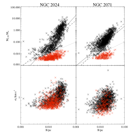
Figure 21: $M_{\rm LTE}-R$ (top panels) and $\sigma_{\rm v}-R$ (bottom panels) relations for NGC 2024 (left) and NGC 2071 (right). Condensations with $M_{\rm LTE}/\hbox{M${}_{\odot}$}<R/{\rm pc}$ are plotted in red because they appear to form a separate population. In the top panels the dotted lines show $M_{\rm LTE}/\hbox{M${}_{\odot}$}=R/{\rm pc}$, the dashed lines show $M_{\rm LTE}\propto R^{2}$ (Larson’s Law), and the solid lines show the lines of best fit: $M_{\rm LTE}\propto R^{2.6}$ for NGC 2024 and $\propto R^{1.7}$ for NGC 2071.

In Fig. 21 we plot the $M_{\rm LTE}-R$ and $\sigma_{\rm v}-R$ relations for both clouds. In the plots of $M_{\rm LTE}$ versus $R$, there appears to be a separate population of low-mass condensations. These low-mass condensations are roughly separated by the line $M_{\rm LTE}/\hbox{M${}_{\odot}$}=R/{\rm pc}$ and are plotted in red. The remaining condensations (plotted in black) appear to have a strong correlation between mass and radius, with correlation coefficients of 0.8 for both clouds. The linear regression coefficient ($s_{xy}/s_{xx}$) of $\log(M_{\rm LTE}/\hbox{M${}_{\odot}$})$ versus $\log(R/{\rm pc})$ is 2.6 for NGC 2024 and 1.7 for NGC 2071, implying that the mass-radius relationship is of the form $M_{\rm LTE}/\hbox{M${}_{\odot}$}\propto(R/{\rm pc})^{\sim 2.6}$ and $\propto(R/{\rm pc})^{\sim 1.7}$ for NGC 2024 and NGC 2071 respectively. Given the scatter in the plots and the uncertainties in the values of $M_{\rm LTE}$ and $R$, the relation for both clouds is consistent with the one found by Kramer, Stutzki & Winnewisser (1996) for their ¹³CO condensations in the southern part of Orion B, which had a power law index of 2.2. The relations are also consistent with Larson’s Law relating mass and radius, which is of the form $M_{\rm LTE}\propto R^{2}$ (Larson, 1981). In Fig. 21 the linear regression fits are shown with the solid black line, and the Larson relation is shown with the broken line.

The distinct population of low-mass condensations, on the other hand, only have a weak correlation between mass and radius (with correlation coefficients of 0.5 in both clouds). Since these populations have such low masses and behave differently to the rest of the condensations it is possible they have some contamination from noise or they may be a population of transient objects in the ambient cloud, not related to the active star formation.

The plots of the velocity dispersion against radius in Fig. 21 do not show an obvious correlation. This is reflected in the low values of the correlation coefficients (0.2 for each cloud). In these plots the populations of low-mass condensations mentioned above are also plotted in red, but here they are not distinct from the other condensations. Several other surveys have also found very weak or no correlation between $\sigma_{\rm v}$ and $R$ for condensations in molecular clouds (e.g. Kramer et al., 1996; Onishi et al., 2002). For a larger range of molecular cloud sizes, Larson (1981) found that $\sigma_{\rm v}\propto R^{\sim 0.4}$. The lack of correlation found here could be because of the small range in $R$ and $\sigma_{\rm v}$ and the large scatter in the values.

Fig. 22 shows the relationship between $M_{\rm vir}$ and $M_{\rm LTE}$. Again, the low-mass condensations identified above are plotted in red, and they appear as a distinct population in this plot. The rest of the condensations are relatively well-correlated, with correlation coefficients of 0.9 for NGC 2024 and 0.8 for NGC 2071. The plots appear to be well-fitted with a power law (solid line), $M_{\rm vir}\propto M_{\rm LTE}^{\beta}$, with $\beta=0.4$ for NGC 2024 and 0.6 for NGC 2071, calculated from the regression coefficient in log-log space. Ikeda, Kitamura & Sunada (2009) found $M_{\rm vir}/M_{\rm LTE}\propto M_{\rm LTE}^{-0.33}$ for H¹³CO⁺ condensations in Orion B (i.e. $\beta=0.67$), which is very close to our value for NGC 2071. The dotted line on each plot shows where the condensations are in approximate equipartition ($M_{\rm vir}=M_{\rm LTE}$). The condensation virial masses are in fact all much higher than their LTE masses, implying that the condensations are unbound. However, there are large uncertainties in both the virial and LTE masses (because of, for example, uncertainties in the distances to the cloud, the fractional abundance of ¹³CO, the excitation temperature, and the assumed density profile), therefore we cannot make any definite conclusions about the fate of any particular condensation from this plot. However, the relative positions of the condensations to each other should be more robust and suggests that condensations from the low-mass population (in red) are in general less bound than the rest (i.e. they have higher $M_{\rm vir}/M_{\rm LTE}$ ratios).

5.3 Condensation mass function

The differential condensation (or core) mass function (CMF) is usually fitted by the power law

$$\frac{dN}{dM}\propto M^{-\alpha}.$$ (20)

If these condensations are the direct precursors of stars, the form of the CMF may provide insights into the origin of the stellar initial mass function (IMF), which is described by Equation 20 with $\alpha=2.35$ (Salpeter, 1955) over a large range of environments. For instance the similarity of the CMF to the IMF for the earliest stages of protostellar evolution, may rule out models of star formation where the shape of the CMF is set at later stages (e.g. Bate & Bonnell, 2005).

Fig. 23 compares the plots of $dN/dM$ versus $M_{\rm LTE}$ for both clouds. The crosses mark the mass function including all of the condensations and the diamonds mark the mass function with the population of low-mass condensations, discussed in Sec. 5.2, removed. The errors plotted show the statistical uncertainties of $\sqrt{N}$, where $N$ is the sample number in each mass bin. The two mass functions for each cloud are the same for $M_{\rm LTE}\ga 0.02~{}\hbox{M${}_{\odot}$}$. Below this mass, the total mass function continues to increase with decreasing mass, whereas the mass function with the low-mass population removed has a turning point and begins to decrease with decreasing mass. Due to the increasing incompleteness in the mass function at these low masses arising from our detection thresholds, we have only attempted to fit the mass function for $M_{\rm LTE}\ga 0.02~{}\hbox{M${}_{\odot}$}$.

Reduced-squared fitting of a single power law mass function to NGC 2024 gives $\alpha\sim 1.3$ for $M_{\rm LTE}\ga 0.02~{}\hbox{M${}_{\odot}$}$ (plotted with the dashed line on Figure 23). The data suggest that there is a break in the power law at $M_{\rm LTE}\sim 2.0~{}\hbox{M${}_{\odot}$}$. Fitting a double power law gives $\alpha_{\rm low}\sim 1.0$ for $0.02<M_{\rm LTE}/\hbox{M${}_{\odot}$}<2.0$ and $\alpha_{\rm high}\sim 2.6$ for $M_{\rm LTE}>2~{}\hbox{M${}_{\odot}$}$.

For NGC 2071, a single power law gives $\alpha\sim 1.7$ for $M_{\rm LTE}\ga 0.02~{}\hbox{M${}_{\odot}$}$, but it is clear that the mass function flattens off for $0.02<M_{\rm LTE}/\hbox{M${}_{\odot}$}<0.12$. Fitting a double power law gives $\alpha_{\rm low}\sim 0.06$ for $0.02<M_{\rm LTE}/\hbox{M${}_{\odot}$}<0.12$ and $\alpha_{\rm high}\sim 2.3$ for $M_{\rm LTE}>2\hbox{M${}_{\odot}$}$. The data suggest there could be another break in the power law at $M_{\rm LTE}\sim 1.0~{}\hbox{M${}_{\odot}$}$.

The single power law values for $\alpha$ are similar to the values of $1.6-1.8$ derived using isotopologues of CO by Kramer et al. (1998) for seven molecular clouds, including Orion B South. For the double power law fits, the values of $\alpha_{\rm high}$ are similar to those derived by J01 for the dust condensation of Orion B North and by Ikeda et al. (2009) for the H¹³CO⁺ condensations of Orion B, which had values of ranging from 2.3 to 3.0. These values are also very similar to the slope of the initial mass function ($\alpha=2.35$), which has been interpreted as evidence for a physical link between the CMF and IMF.

Ikeda et al. (2009) also found $\alpha_{\rm low}\sim 0.06$, just as we have found for NGC 2071. They suggested the flattening could be a confusion effect where low-mass cores are misidentified as parts of high-mass cores. The turnover point found by Ikeda et al. (2009) was much higher however, at $6~{}\hbox{M${}_{\odot}$}$, compared to our value of $0.12~{}\hbox{M${}_{\odot}$}$. Again this could be because the ¹³CO LTE masses are underestimated due to opacity and freeze-out.

From our analysis on the ¹³CO condensations in NGC 2024 and NGC 2071, we have found that NGC 2024 has a wider mass range than NGC 2071 (with masses up to $\sim 13~{}\hbox{M${}_{\odot}$}$ for NGC 2024, compared to $\sim 5~{}\hbox{M${}_{\odot}$}$ for NGC 2071). Compared to the virial masses and condensation masses derived from other tracers, the ¹³CO mass estimates appear to be underestimated, possibly due to optical depth and freeze-out effects. The relationships between the condensation properties are similar to those seen in previous surveys of condensations of CO isotopologues and H¹³CO⁺. The slopes of the CMF at the high-mass ends ($\sim 2.6$ for NGC 2024 and $\sim 2.3$ for NGC 2071) are very similar to the slope of the initial mass function.

Figure 22: Plots of virial mass versus LTE mass for NGC 2024 (left) and NGC 2071 (right). Condensations with $M_{\rm LTE}/\hbox{M${}_{\odot}$}<R/{\rm pc}$ are plotted in red. The solid lines on each plot show the lines of best fit ($M_{\rm vir}\propto M_{\rm LTE}^{0.4}$ for NGC 2024 and $\propto M_{\rm LTE}^{0.6}$ for NGC 2071) and the dotted lines show $M_{\rm vir}=M_{\rm LTE}$.

Figure 23: The differential mass functions of ¹³CO condensations in NGC 2024 (left) and NGC 2071 (right). The crosses mark the mass function including all of the condensations and the diamonds mark the mass function with condensations with $M_{\rm LTE}/\hbox{M${}_{\odot}$}<R/{\rm pc}$ removed. The errors plotted show the statistical uncertainties of $\sqrt{N}$, where $N$ is the sample number in each mass bin. The dashed lines show the single power law fits ($\alpha=1.3$ for NGC 2024 and $\alpha=1.7$ for NGC 2071), and the solid lines show the double power law fits ($\alpha_{\rm low}=1.0$ for $0.02<M_{\rm LTE}/\hbox{M${}_{\odot}$}<2.0$ and $\alpha_{\rm high}=2.6$ for $M_{\rm LTE}>2\hbox{M${}_{\odot}$}$ for NGC 2024 and $\alpha_{\rm low}=0.06$ for $0.02<M_{\rm LTE}/\hbox{M${}_{\odot}$}<0.12$ and $\alpha_{\rm high}=2.3$ for $M_{\rm LTE}>2\hbox{M${}_{\odot}$}$ for NGC 2071).

6 Summary

We have offered a first look at the data on Orion B being collected by HARP/ACSIS on the JCMT for the Gould Belt Legacy Survey. Our observations of CO, ¹³CO and C¹⁸O $J=3\rightarrow 2$ provide a comprehensive determination of the characteristic physical properties and dynamics of star forming regions. We have observed two large regions in Orion B, (10.8$\times$22.5) arcmin² in NGC 2024, and (13.5$\times$21.6) arcmin² in NGC 2071. Towards NGC 2024, ¹²CO and ¹³CO are detected throughout the region, while C¹⁸O is detected in an extended ridge, which follows the dust emission, and also in a fragmented ring surrounding a bright optical nebula. The ¹²CO line profiles indicate multiple line of sight components. Comparisons of the intensity ratios of the three isotopologues indicate that the ¹²CO is optically thick throughout the cloud, and also in the lower-velocity outflow material, while the C¹⁸O is generally optically thin. These opacity results also apply to NGC 2071.

Towards NGC 2071, the molecular gas is concentrated in a region almost completely surrounding a bright optical nebula. The ¹²CO emission is heavily self-absorbed, and ¹³CO also shows self-absorption in the densest regions. The main outflow is very energetic, and is seen to produce extended wings even in the C¹⁸O line profiles.

Both clouds show a complex clumpy and filamentary structure. In the regions traced by C¹⁸O, the equivalent widths suggest the bulk of the quiescent material has a lower velocity dispersion than the material in which it is embedded, increasing only in the regions of current star formation. The energetic outflow activity is contributing a few percent of the kinetic energy of NGC 2024, while the outflows dominate the kinetic energy towards NGC 2071. Towards NGC 2024, the low-velocity red-shifted material is extended and filamentary, while the low-velocity blue-shifted material is clumpy and compact.

A CLUMPFIND analysis on the ¹³CO data finds multiple ¹³CO condensations spatially associated with SCUBA dust cores, $\sim$7.4 towards NGC 2024, and $\sim$3.7 towards NGC 2071. The condensations in NGC 2024 have higher LTE and virial masses than in NGC 2071, and towards both clouds, $M_{\rm vir}\geq M_{\rm LTE}$. The slopes of the condensations’ mass function at the high-mass ends are in agreement with the slope of the initial mass function. Towards NGC 2024, we also detect a group of condensations that appear to be less bound, which may be tracing transient clumps that do not go on to form stars.

These data are still being collected, and the Gould Belt Survey has a final 1$\sigma$ noise requirement of of 0.3 K in 1.0 ${\rm km\,s}^{-1}$ for ¹²CO, and 0.3 K in 0.1 ${\rm km\,s}^{-1}$ for C¹⁸O per 7.5 arcsec pixel. ¹³CO is obtained simultaneously with C¹⁸O, and the C¹⁸O requirement sets a 1$\sigma$ noise level of 0.25 K in 0.1 ${\rm km\,s}^{-1}$ for ¹³CO. When the full HARP data set has been obtained, we will carry out more detailed analyses of the individual cores and outflow properties in the Orion B clouds. The completeness limit for the ¹³CO results will be improved, although overall condensation masses, and the slope of the condensations’ mass function will not be significantly affected. With datasets of the same sensitivity, the properties of the Orion B clouds will be compared to the other star-forming clouds being observed by the GBS. This data set will be highly complementary to the SCUBA-2 and POL-2 observations planned as part of this survey, and to planned Herschel key programmes.

References

- Anthony-Twarog (1982) Anthony-Twarog B.J., 1982, AJ, 87, 1213
- Aspin et al. (1992) Aspin C., Sandell G., Walther D.M., 1992, MNRAS, 258, 684
- Bally (2009) Bally J., 2009, in Reiputh B., ed, Handbook of Star Forming Regions Vol. I: The Northern Sky, p. 459
- Barnes et al. (1989) Barnes P.J., Crutcher R.M., Bieging J.H. et al. 1989, ApJ, 342, 883
- Barnes & Crutcher (1990) Barnes P.J., Crutcher R.M., 1990, ApJ, 351, 176
- Bastien et al. (2005) Bastien P., Jenness T., Molnar J., 2005, in Adamson A., Aspin C., Davis C.J., Fujiyoshi T., eds, ASP Conf. Ser. Vol. 343, Astron. Polarimetry: Current Status and Future Directions p.69
- Bate & Bonnell (2005) Bate M.R., Bonnell I.A., 2005, MNRAS, 356, 1201
- Berry et al. (2007) Berry D.S., Reinhold K., Jenness T., Economou F., 2007, in Shaw R.A., Hill F., Bell D.J., eds, ASP Conf. Ser. Vol. 376, Astron. Data Analysis Software and Systems XVI p. 425
- Bertoldi & McKee (1992) Bertoldi F., McKee C.F., 1992, ApJ, 395, 140
- Bik et al. (2003) Bik A., Lenorzer A., Kaper L. et al., 2003, A&A, 404, 249
- Buckle et al. (2009) Buckle J.V., Hills R.E., Smith H. et al., 2009, MNRAS, accepted
- Burke & Hollenbach (1983) Burke J.R., Hollenbach D. J., 1983, ApJ, 265, 223
- Burton et al. (1989) Burton M.G., Geballe T.R., Brand P.W.J.L., 1989, MNRAS, 238, 1513
- Butner et al. (1990) Butner H.M., Evans N.J., Harvey P.M., Mundy L.G., Natta A., Randich M.S., 1990, ApJ, 364, 164
- Chernin & Masson (1992) Chernin L.M., Masson C.R., 1992, ApJ, 396, L35
- Chernin & Welch (1995) Chernin L.M., Welch W.J., 1995, ApJ, 440, L21
- Chernin (1996) Chernin L.W., 1996, ApJ, 460, 711
- Comerón et al. (1996) Comerón F., Rieke G.H., Rieke M.J., 1996, ApJ, 473, 294
- Currie et al. (2008) Currie, M.J., Draper, P.W., Berry D.S., Jenness T., Cavanagh B., Economou F., 2008, in Argyle R.W., Bunclark P.S., Lewis J.R., eds, ASP Conf. Ser. Vol. 394, Astron. Data Analysis Software and Systems p. 650
- Curtis et al. (2009) Curtis E.I., Richer J.S., Buckle J.V., 2009, MNRAS, submitted
- Dent et al. (2000) Dent W., Duncan W., Ellis M. et al. 2000, in Mangum J.G., Radford S.J.E., eds, ASP Conf. Ser. Vol. 217, Imaging at Radio through Submillimeter Wavelengths p. 33
- Dobashi et al. (2005) Dobashi K., Uehara H., Kandori R., Sakurai T., Kaiden M., Umemoto T., Sato F., 2005, PASJ, 57, 1
- Dotson et al. (2000) Dotson J.L., Davidson J., Dowell C.D., Schleuning D.A., Hildebrand R.H., 2000, ApJS, 128, 335
- Di Francesco et al. (2008) Di Francesco J., Johnstone D., Kirk H., MacKenzie T., Ledwosinska E., 2008, ApJS, 175, 277
- Eislöffel (2000) Eislöffel J., 2000, A&A, 354, 236
- Emprechtinger et al. (2009) Emprechtinger M., Wiedner M.C., Simon R. et al., 2009, A&A, 496, 731
- Flaherty & Muzerolle (2008) Flaherty K.M., Muzerolle J., 2008, AJ, 135, 966
- Frerking et al. (1982) Frerking M.A., Langer W.D., Wilson R.W., 1982, ApJ, 262, 590
- Garden et al. (1990) Garden R.P., Russell A.P.G., Burton M.G., 1990, ApJ, 354, 232
- Garden et al. (1991) Garden R. P., Hayashi M., Hasegawa T., Gatley I., Kaifu N., 1991, ApJ, 374, 540
- Giannini et al. (2000) Giannini T., Nisini B., Lorenzetti D. et al., 2000, A&A, 358, 310
- Gibb (2009) Gibb A.G., 2009, in Reiputh B., ed, Handbook of Star Forming Regions Vol. I: The Northern Sky, p. 693
- Graf et al. (1993) Graf U.U, Eckart A., Grenzel R., Harris A.I., Poglitsch A., Russell A.P.G., Stutzki J., 1993, ApJ, 405, 249
- Greaves et al. (2001) Greaves J.S., Holland W.S., Ward-Thompson D., 2001, ApJ, 546, L53
- Haisch et al. (2000) Haisch K.E., Lada E.A., Lada C.J., 2000, AJ, 120, 1396
- Hildebrand et al. (1995) Hildebrand R.H., Dotson J.L., Dowell C.D., Platt S.R., Schleuning D., Davidson J.A., Novak G., 1995, in Haas M.R., Davidson J.A., Erickson E.F., eds, ASP Conf. Ser. Vol. 73, Airborne Astron. Symp. on the Galactic Ecosystem: From Gas to Stars to Dust p. 97
- Holland et al. (2006) Holland W.S., MacIntosh M., Fairley A. et al., 2006, in Zmuidzinas J., Holland W. S., Withington S. Duncan W.D., eds, Proc. SPIE Vol. 6275, SCUBA-2: a 10,000-pixel submillimeter camera for the James Clerk Maxwell Telescope, SPIE, Bellingham, p. 45
- Houde et al. (2001) Houde M., Phillips T.G., Bastien P., Peng R., Yoshida H., 2001, ApJ, 547, 311
- Ikeda et al. (2009) Ikeda N., Kitamura Y., Sunada K., 2009, ApJ, 691,1560
- Jenness et al. (2008) Jenness T., Cavanagh B., Economou F., Berry D.S., 2008, in Argyle R.W., Bunclark P.S., Lewis J.R., eds, ASP Conf. Ser. Vol. 394, Astron. Data Analysis Software and Systems p. 565
- Johnstone et al. (2001) Johnstone D., Fich M., Mitchell G.F., Moriarty-Schieven G., 2001, ApJ, 559, 307 (J01)
- Johnstone et al. (2006) Johnstone D., Matthews H., Mitchell G.F., 2006, ApJ, 639, 259 (J06)
- Kandori et al. (2007) Kandori R., Tamura M., Kusakabe N. et al., 2007, PASJ, 59, 487
- Kitamura et al. (1990) Kitamura Y., Kawabe R., Yamashita T., Hayashi M., 1990, ApJ, 363, 180
- Kramer et al. (1998) Kramer C., Stutzki J., Rohrig R., Corneliussen U., 1998, A&A, 329, 249
- Kramer et al. (1996) Kramer C., Stutzki J., Winnewisser G., 1996, A&A, 307, 915
- Krügel et al. (1982) Krügel E., Thum C., Pankonin V., Martin-Pintado J., 1982, A&AS, 48, 345
- Kutner & Ulich (1981) Kutner M.L., Ulich B.L., 1981, ApJ, 250, 341
- Kutner et al. (1977) Kutner M.L., Tucker K.D., Chin G., Thaddeus P., 1977, ApJ, 215, 521.
- Lada et al. (1991) Lada E.A., Bally J., Stark A.A., 1991, ApJ, 368, 432
- Lada et al. (1991) Lada E.A., DePoy D.L., Evans N.J., Gatley I., 1991, ApJ, 371, 1
- Ladd et al. (1998) Ladd E.F., Fuller G.A., Deane J.R., 1998, ApJ, 495, 871
- Lane & Bally (1986) Lane A.P., Bally J., 1986, ApJ, 310, 820
- Larson (1981) Larson, R. B., 1981, MNRAS, 194, 809
- Lis et al. (1999) Lis D.C., Menten K., Zylka R., 1999, ApJ, 527, 856
- MacLaren et al. (1988) MacLaren I., Richardson K.M., Wolfendale A.W., 1988, ApJ, 333, 821
- Maddalena et al. (1986) Maddalena R.J., Morris M., Moscowitz J., Thaddeus P., 1986, ApJ, 303, 375
- Mangum et al. (1999) Mangum J.G., Wootten A., Barsony M,. 1999, ApJ, 526, 845
- Mangum & Wootten (1993) Mangum J.G., Wootten A., 1993, ApJS, 89, 123
- Margulis & Snell (1989) Margulis M., Snell R.L., 1989, ApJ, 343, 779
- Matthews et al. (2002) Matthews B.C., Fiege J.D., Moriarty-Schieven G., 2002, ApJ, 569, 304
- Menten et al. (2007) Menten K.M., Reid M.J., Forbrich J., Brunthaler A., 2007, A&A, 474, 515
- Meyer (2009) Meyer M., 2009, in Reiputh B., ed, Handbook of Star Forming Regions Vol. I: The Northern Sky, p. 662
- Mezger et al. (1988) Mezger P.G., Chini R., Kreysa E., Wink J.E., Salter C.J., 1988, A&A, 191, 44
- Mezger et al. (1992) Mezger P.G., Sievers A.W., Haslam C.G.T., Kreysa E., Lemke R., Mauersberger R., Wilson T.L., 1992, A&A, 256, 631
- Mitchell et al. (2001) Mitchell G.F., Johnstone D., Moriarty-Schieven G., Fich M., Tothill N.F.H., 2001, ApJ, 556, 215
- Moriarty-Schieven et al. (1989) Moriarty-Schieven G.H., Hughes V.A., Snell R.L., 1989, ApJ, 347, 358
- Motte et al. (2001) Motte F., André P., Ward-Thompson D., Bontemps S., 2001, A&A, 372, L41
- Myers et al. (1983) Myers P.C., Linke R.A., Benson P.J., 1983, ApJ, 264, 517
- Onishi et al. (2002) Onishi T., Mizuno A., Kawamura A., Tachihara K., Fukui Y., 2002, ApJ, 575, 950
- Persson et al. (1981) Persson S.E., Geballe T.R., Simon T. et al. 1981, ApJ, 251, L85
- Pineda et al. (2008) Pineda J.E., Caselli P., Goodman A.A., 2008, ApJ, 679, 481
- Phillips et al. (1982) Phillips J.P., White G.J., Ade P.A.R., 1982, A&A, 116, 130
- Phillips et al. (1988) Phillips J.P., White G.J., Rainey R. et al. 1988, A&A, 190, 289
- Richer et al. (1989) Richer J.S., Hills R.E., Padman R., Russell A.P.G., 1989, MNRAS, 241, 231
- Richer et al. (1992) Richer J.S., Hills R.E., Padman R., 1992, MNRAS, 254, 525
- Rodríguez et al. (2003) Rodríguez L.F., Gómez Y., Reipurth B., 2003, ApJ, 598, 1100
- Scoville et al. (1986) Scoville N.Z., Sargent A.I., Sanders D.B., Claussen M.J., Masson C.R., Lo K.Y., Phillips T.G., 1986, ApJ, 303, 416
- Salpeter (1955) Salpeter E.E., 1955, ApJ, 121, 161
- Seth et al. (2002) Seth A.C., Greenhill L.J., Holder B.P., 2002, ApJ, 581, 325
- Smith et al. (2003) Smith H., Hills R.E., Withington S. et al., 2003, in Phillips T.G., Zmuidzinas J. eds, Proc. SPIE Vol. 4855, Millimeter and Submillimeter Detectors for Astronomy, SPIE, Bellingham, p. 338
- Smith et al. (2008) Smith H., Buckle J.V., Hills R.E. et al. 2008, in Duncan W.D., Holland W.S., Withington S., Zmuidzinas J., eds, Proc. SPIE Vol.7020, HARP: a submillimetre heterodyne array receiver operating on the James Clerk Maxwell Telescope, SPIE, Bellingham, p. 24
- Smith & Beck (1994) Smith H.A., Beck S.C., 1994, ApJ, 420, 643
- Snell & Bally (1986) Snell R.L., Bally J., 1986, ApJ, 303, 683
- Snell et al. (1984) Snell R.L., Scoville N.Z., Sanders D.B., Erickson N.R., 1984, ApJ, 284, 176
- Snell et al. (2000) Snell R.L., Howe J.E., Ashby M.L.N. et al., 2000, ApJ, 539, L101.
- Stojimirovic et al. (2008) Stojimirovic I., Snell R.L., Narayanan G. 2008, ApJ, 679, 557
- Tothill & Mitchell (2001) Tothill N.F.H., Mitchell G.F., 2001, in Pilbratt, G. L. et al., eds., The Promise of the Herschel Space Observatory, ESA-SP 460, p. 503
- Torrelles et al. (1998) Torrelles J.M., Gómez J.F., Rodríguez L.F., Curiel S., Anglada G., Ho P.T.P., 1998, ApJ, 505, 756
- Tucker et al. (1973) Tucker K.D., Kutner M.L., Thaddeus P., 1973, ApJ, 186, L13
- Visser et al. (1998) Visser A.E., Richer J.S., Chandler C.J., Padman R., 1998, MNRAS, 301, 585
- Walther et al. (1993) Walther D.M., Robson E.I., Aspin C., Dent W.R.F., 1993, ApJ, 418, 310
- Ward-Thompson et al. (2007) Ward-Thompson D., Di Francesco J., Hatchell J. et al., 2007, PASP, 119, 855
- Watt et al. (1979) Watt G.D., White G.J., Cronin N.J., van Vliet A.H.F., 1979, MNRAS, 189, 287
- White & Phillips (1981) White G.J., Phillips J.P., 1981, MNRAS, 194, 947
- White et al. (1981) White G.J., Phillips J.P., Watt G.D., 1981, MNRAS, 197, 745
- Williams et al. (1994) Williams J.P., de Geus E.J., Blitz L., 1994, ApJ, 428, 693
- Wilson (1999) Wilson T.L. 1999, Rep. Prog. Phys., 62, 143
- Wilson et al. (2005) Wilson B. A., Dame T. M., Masheder M.R.W., Thaddeus P., 2005, ApJ, 430, 523