Primordial Non-Gaussianities from the Trispectra in Multiple Field Inflationary Models

Abstract:

We investigate the primordial non-Gaussianities from the trispectra in multi-field inflation models, which can be seen as generalization of multi-field $k$-inflation and multi-DBI inflation. We derive the full fourth-order perturbation action for the inflaton fields and evaluate the four-point correlation functions for the perturbations in the limit $c_{\textrm{a}}\ll 1$ and $c_{\textrm{e}}\ll 1$. There are three types of momentum-dependent shape functions which arise from three types of four-point interaction vertices. The final trispectrum of the curvature perturbation can be expressed in terms of the deformations and permutations of these three shape functions, and is determined by $c_{\textrm{a}}$, $c_{\textrm{e}}$, $\lambda$ , $\Pi$ which depend on the non-linear structure of the model and also the transfer function $T_{\mathcal{R}\mathcal{S}}$. We also discuss the parameter space for the trispectrum and plot the shape diagrams for the trispectrum both for visualization and for distinguishing different shapes from each other.

1 Introduction

Current observational data support cosmological inflation greatly [1], in which primordial perturbations assumed responsible for Cosmic Microwave Background anisotropies and Large-Scale Structure formation are generated from quantum fluctuations and stretched to superhorizon scales during inflation (see e.g. [3] for a review). Actually, inflation itself is not a single model, but rather a theoretical framework. One of the most robust predictions of inflation is the almost scale-invariant, Gaussian and adiabatic primordial fluctuation. However, from the point of view of power spectrum (i.e., Fourier transformation of the tree-level two-point equal-time correlation function) of the cosmological perturbation, many inflation models are “degenerate”. The theory and observation of power spectrum do not give us an unique theory of inflation. Phenomena beyond linear-order have been extensively investigated over the past several years.

The most significant progress beyond power spectrum is the investigation of statistical non-Gaussianities of CMB anisotropies and primordial fluctuations [2] (see e.g. [9] for a nice review). From the field theoretical point of view, non-Gaussianity describes interactions among perturbations, which will cause non-vanishing higher-order correlation functions. Such interactions are mandatory in any realistic inflationary models, which come from both the non-linear nature of gravitation and the self-interactions of inflation field(s). In standard slow-roll inflation scenario, however, the non-Gaussianities have been proved too small to be detected [7] (see also [8]), even with PLANCK satellite [10]. Thus, any detection of non-Gaussianities would not only rule out the simplest inflation models but also give us valuable insight into fundamental physics of inflation [11, 12, 13, 14, 15, 16, 17, 18, 19].

Generally speaking, primordial non-Gaussianities can be large, if one or more of the following four conditions are violated: 1) slow-roll conditions, 2) canonical kinetic terms, 3) single field and 4) Bunch-Davies vacuum [9]. For single-field models, for example, various possibilities have been investigated in order to generate large non-Gaussianities by introducing complicated kinetic terms [20, 21, 22, 23, 24, 25, 26, 27, 28, 29, 30, 31, 32] which belong to the more general class of $k$-inflation models [44, 45], in which the small-speed of sound $c_{s}\ll 1$ enhances the derivative-coupling of perturbations, or other mechanisms which enhance the interactions during inflation or non-linearities during superhorizon evolution [33, 34, 35, 36, 37, 38, 39, 40, 41, 42, 43].

From the point of view of data analysis, there are two typical types of non-Gaussianities which are most interesting: the so-called “local” type and the “equilateral” type. The former describes the strength of modulations of short wavelength perturbation modes by long wavelength modes, while the later describes the correlations among modes with similar wavelengthes. It has been clear from the studies of non-Gaussianities in single-field models that, single-field inflationary models with non-canonical kinetic terms can have large “equilateral”-type non-Gaussianities, since the “derivative-coupled” interactions among different modes are enhanced by the non-canonical structure of the kinetic term. While single-field models can never generate large “local”-type non-Gaussianities, unless the generalized slow-roll conditions are abandoned.

Multiple field inflationary models provide us with more possibilities to generate large non-Gaussianities during inflation [57, 58, 59, 60, 61, 62, 63, 64, 65, 55, 56, 67, 68, 69, 70, 71, 72, 73, 74, 86, 87]. It has been shown that multi-inflaton models with non-canonical kinetic terms are also mainly characterized by equilateral-type non-Gaussianities rather than local-type. Local-type non-Gaussianities can be generated during superhorizon evolution of cosmological perturbations, for example in inhomogeneous “end-of-inflation” models [75, 76, 77, 79, 78] or curvaton scenario [94, 95, 96, 97, 98, 99, 100, 101].

In this work, we investigate primordial non-Gaussianities from the trispectra (i.e. Fourier transformation of equal-time four-point correlation functions) of cosmological perturbations in general multiple field models. We consider the model with general scalar-fields Lagrangian of the form $P(X^{IJ},\phi^{I})$. This form of Lagrangian was first investigated in [58, 62]. It includes single-field models with non-canonical kinetic term [44, 45], multi-field k-inflation [73, 60] and multi-field DBI models [57, 58, 61, 64] as special cases, and thus deserves detailed studies. Bispectrum in general multi-field models with small speed of sound has been investigated in [57, 58, 60, 62]. Trispectra in single-field models have been investigated by various author [22, 26, 27, 28, 29, 30, 31, 32] and in multi-field models until very recently [61, 64, 65, 66].

We start from the the full fourth-order action for the scalar perturbations and then evaluate the leading-order four-point functions around sound-horizon crossing in the approximation $c_{\textrm{a}}\ll 1$ and $c_{\textrm{e}}\ll 1$, where $c_{\textrm{a}}$ and $c_{\textrm{e}}$ are propagation speeds of adiabatic and entropy modes respectively. In this work we restrict the calculations to the contributions from the so-called “contact interaction”, i.e. the contributions from the “four-point direct interaction vertices”. As in the case in general single-field models, in the leading-order, we find three fundamental shape functions $A_{1}(k_{1},k_{2},k_{3},k_{4})$, $A_{2}(k_{1},k_{2};\bm{k}_{1},\bm{k}_{2})$ and $A_{3}(\bm{k}_{1},\bm{k}_{2};\bm{k}_{3},\bm{k}_{4})$, corresponding to three different types of four-point interaction vertices. Moreover, in addition to the pure adiabatic four-point function $\left\langle Q_{\sigma}Q_{\sigma}Q_{\sigma}Q_{\sigma}\right\rangle$, there also exist pure entropy four-point function $\left\langle Q_{s}Q_{s}Q_{s}Q_{s}\right\rangle$ and one mixed contribution $\left\langle Q_{\sigma}Q_{\sigma}Q_{s}Q_{s}\right\rangle$ (we denote $Q_{\sigma}$ and $Q_{s}$ as the adiabatic and entropy modes respectively). The four-point correlation functions $\left\langle Q_{\sigma}Q_{\sigma}Q_{\sigma}Q_{\sigma}\right\rangle$, $\left\langle Q_{\sigma}Q_{\sigma}Q_{s}Q_{s}\right\rangle$ and $\left\langle Q_{s}Q_{s}Q_{s}Q_{s}\right\rangle$ can be generally written in terms of various deformations and permutations of these three types of shape functions. Since the observable is the curvature perturbation $\mathcal{R}$, we also investigate the trispectrum of the curvature perturbation $\left\langle\mathcal{R}\mathcal{R}\mathcal{R}\mathcal{R}\right\rangle$ on large scales.

In this work, we assume the propagation speeds of adiabatic mode and entropy modes be different: $c_{\textrm{a}}\neq c_{\textrm{e}}$. Thus, unlike the multi-field DBI models [57, 58, 61, 64] where $c_{\textrm{a}}=c_{\textrm{e}}=c_{s}$ and we can abstract common shape functions for both $\left\langle Q_{\sigma}Q_{\sigma}Q_{\sigma}\right\rangle$ and $\left\langle Q_{\sigma}Q_{s}Q_{s}\right\rangle$, in this work we will see that $c_{\textrm{a}}$, $c_{\textrm{e}}$ enter the definition of the shape function intrinsically. More precisely, as we will see, the trispectrum of the curvature perturbation is determined by four parameters $c_{\textrm{a}}$, $c_{\textrm{e}}$, $\lambda$, $\Pi$ which arise from the non-linear structure of the theory and also $T_{\mathcal{R}\mathcal{S}}$ which characterizes the transfer from entropy modes to adiabatic modes during superhorizon evolution.

This paper is organized as follows. In section 2, we describe the model and set up the perturbation theory in spatially-flat gauge, then we briefly review the linear perturbation and the power spectra in section 3. In section 4, we give the full fourth-order perturbation action and derive the interaction Hamiltonian in the interaction picture. And we calculate the four-point functions and the trispectra in section 5. In section 6, we give a general discussion on characterizing the trispectrum and we plot the shape diagrams and investigate the non-linear parameters. In the end we make a conclusion and discuss some related issues.

In this paper, we choose $c=\hbar=M_{\textrm{pl}}\equiv\frac{1}{8\pi G}=1$.

2 Basic Setup

2.1 Model and Background

In this work we consider a general class of multi-field models containing $\mathcal{N}$ scalar fields coupled to Einstein gravity. The action takes the form

$${}S=\int d^{4}x\,\sqrt{-g}\left[\frac{R}{2}+P\left(X^{IJ},\phi^{I}\right)\right]\,,$$ (1)

where $\phi^{I}$ ($I=1,2,\cdots,\mathcal{N}$) are scalar fields acting as inflaton fields, and

$$X^{IJ}\equiv-\frac{1}{2}g^{\mu\nu}\partial_{\mu}\phi^{I}\partial_{\nu}\phi^{J}\,,$$ (2)

is the kinetic term (matrix), $g_{\mu\nu}$ is the spacetime metric tensor with signature $(-,+,+,+)$. “$I,J$”-indices are raised, lowered and contracted by $\mathcal{N}$-dimensional field-space metric $G_{IJ}=G_{IJ}(\phi^{I})$. This form of Lagrangian includes multi-field k-inflation and multi-DBI models as special cases.

Modern “action approach” of cosmological perturbations is based on the ADM formalism of gravitation, in which spacetime metric is written as

$$ds^{2}=-N^{2}dt^{2}+h_{ij}(dx^{i}+N^{i}dt)(dx^{j}+N^{j}dt)\;,$$ (3)

with $N=N(t,\bm{x})$ is the lapse function and $N_{i}=N_{i}(t,\bm{x})$ is the shift vector, $h_{ij}$ is the spatial metric on constant time hypersurfaces. The ADM formalism is convenient because the equations of motion for $N$ and $N^{i}$ are exactly the energy and momentum constraints which are easy to solve. Under the ADM formalism, the action (1) can be written as (up to total derivative terms)

$${}S=\int dtd^{3}x\,\sqrt{h}N\left(\frac{1}{2}R^{(3)}+\frac{1}{2N^{2}}\left(E_{ij}E^{ij}-E^{2}\right)\right)+\int dtd^{3}x\,\sqrt{h}N\,P\,,$$ (4)

where $h\equiv\det h_{ij}$ and the symmetric tensor

$$E_{ij}\equiv\frac{1}{2}\left(\dot{h}_{ij}-\nabla_{i}N_{j}-\nabla_{j}N_{i}\right)\,,$$ (5)

with $\nabla_{i}$ is the spatial covariant derivative defined with spatial metric $h_{ij}$ and $E\equiv\mathrm{tr}E_{ij}=h^{ij}E_{ij}$. $R^{(3)}$ is the three-dimensional Ricci scalar which is computed from the spatial metric $h_{ij}$. In ADM formalism, spatial indices are raised and lowered using $h_{ij}$ and $h^{ij}$.

In ADM formalism, the kinetic matrix $X^{IJ}$ can be written as

$$X^{IJ}=-\frac{1}{2}h^{ij}\partial_{i}\phi^{I}\partial_{j}\phi^{J}+\frac{1}{2N^{2}}v^{I}v^{J}\,,$$ (6)

where

$$v^{I}\equiv\dot{\phi}^{I}-N^{i}\nabla_{i}\phi^{I}\,.$$ (7)

2.1.1 Equations of Motion

The equations of motion for the scalar fields are

$$\nabla_{\mu}\left(P_{,\langle IJ\rangle}\partial^{\mu}\phi^{I}\right)+P_{,J}=0\,,$$ (8)

where $\nabla_{\mu}$ is the four-dimensional covariant derivative. Here and in what follows, we denote

$$P_{,\langle IJ\rangle}\equiv\frac{\partial P}{\partial X^{IJ}}\,,\qquad P_{,\langle IJ\rangle\langle KL\rangle}\equiv\frac{\partial^{2}P}{\partial X^{IJ}\partial X^{KL}}\,,$$ (9)

for shorthand.

The equations of motion for $N$ and $N_{i}$ are Hamiltonian and momentum constraints respectively,

$${}R^{(3)}+2P-\frac{2}{N^{2}}P_{,\langle IJ\rangle}v^{I}v^{J}-\frac{1}{N^{2}}\left(E_{ij}E^{ij}-E^{2}\right) =0\,,$$ (10)

$$\nabla_{j}\left(\frac{1}{N}\left(E^{j}_{i}-E\delta^{j}_{i}\right)\right)-\frac{P_{,\langle IJ\rangle}}{N}v^{I}\nabla_{i}\phi^{J} =0\,.$$

2.1.2 Background

In this work, we investigate scalar perturbations around a flat FRW background, the background spacetime metric takes the form

$$ds^{2}=-dt^{2}+a^{2}(t)\delta_{ij}dx^{i}dx^{j}\,,$$ (11)

where $a(t)$ is the so-called scale-factor. The Friedmann equation and the continuity equation are

$$H^{2} =\frac{\rho}{3}\equiv\frac{1}{3}\left(2X^{IJ}P_{,\langle IJ\rangle}-P\right)\,,$$ (12)

$$\dot{\rho} =-3H(\rho+P)\,.$$

In the above equations, all quantities are background values. From the above two equations we can also get another convenient equation

$${}\dot{H}=-X^{IJ}P_{,\langle IJ\rangle}\,.$$ (13)

The background equations of motion for the scalar fields are

$$P_{,\langle IJ\rangle}\ddot{\phi}^{I}+\left(3HP_{,\langle IJ\rangle}+\dot{P}_{,\langle IJ\rangle}\right)\dot{\phi}^{I}-P_{,J}=0\,,$$ (14)

where $P_{,I}$ denotes derivative of $P$ with respect to $\phi^{I}$: $P_{,I}\equiv\frac{\partial P}{\partial\phi^{I}}$.

In this work, we investigate cosmological perturbations during an exponential inflation period. Thus, from (13) it is convenient to define a slow-roll parameter

$$\epsilon\equiv-\frac{\dot{H}}{H^{2}}=\frac{P_{,\langle IJ\rangle}\dot{\phi}_{0}^{I}\dot{\phi}_{0}^{J}}{2H^{2}}\,.$$ (15)

2.2 Perturbation Theory in Spatially-flat Gauge

The scalar metric fluctuations about our background can be written as (see [5, 6] for nice review of the theory of cosmological perturbations)

$$\delta N =\alpha\,,$$ (16)

$$\delta N_{i} =\partial_{i}\beta\,,$$

$$\delta g_{ij} =-2a^{2}\bigl{(}\psi\delta_{ij}-\partial_{i}\partial_{j}E)\,$$

where $\alpha,\beta,\psi$ and $E$ are functions of space and time. The scalar field perturbations are denoted by $\delta\phi^{I}\equiv Q^{I}$.

Before proceeding, we would like to analyze the (scalar) dynamical degrees of freedom in our system. In the beginning we have $\mathcal{N}+4$ apparent scalar degrees of freedom. The diffeomorphism of Einstein gravity eliminates two of them, leaving us $\mathcal{N}+2$ scalar degrees of freedom. Furthermore, two of these $\mathcal{N}+2$ degrees of freedom are non-dynamical. In ADM formalism, these are just the fluctuations $\delta N=\alpha$ and $\delta N_{i}=\partial_{i}\beta$. Thus, there are $\mathcal{N}$ propagating degrees of freedom in our system. As has been addressed, the diffeomorphism invariance allows us to choose convenient gauges to eliminate two degrees of freedom. In single-field models, there are two convenient gauge choices: comoving gauge corresponding to choosing $\delta\phi=E=0$ or spatially-flat gauge corresponding to $\psi=E=0$. In multi-field case, the comoving gauge loses its convenience since we cannot set $\delta\rho=0$ in multi-field case. Thus, in this work we use the spatially-flat gauge.

In the spatially-flat gauge, propagating degrees of freedom for scalar perturbations are the inflaton field perturbations $Q^{I}(t,\bm{x})$, while $\delta N$ and $\delta N_{i}$ are non-dynamical constraints. In this work, we focus on scalar perturbations. The perturbations take the form

$${}\phi^{I}(t,\bm{x}) =\phi_{0}^{I}(t)+Q^{I}(t,\bm{x})\,,$$ (17)

$$h_{ij} \equiv a^{2}\delta_{ij}\,$$

$$N =1+\alpha_{1}+\alpha_{2}+\cdots\,,$$

$$N_{i} =\partial_{i}(\beta_{1}+\beta_{2}+\cdots)+\theta_{1i}+\theta_{2i}+\cdots\,,$$

where $\phi_{0}^{I}(t)$ is the background value, and $\alpha_{n},\beta_{n},\theta_{ni}$ are of order $\mathcal{O}(Q^{n})$.

The next step is to solve the constraints $\alpha_{n}$, $\beta_{n}$ and $\theta_{ni}$ in terms of $Q^{I}$. Fortunately, in order to expand the action to fourth-order in $Q^{I}$, the solutions for the constraints up to the second-order are adequate. In general, we need the solutions for constraints $N$ and $N_{i}$ up to $\mathcal{O}(Q^{[n/2]})$ order ($[n/2]$ means the largest integer $\leq n/2$), if we want to expand the action to $\mathcal{O}(Q^{n})$ order and to calculate the $n$-point correlation functions.

2.2.1 Solving the Constraints

At the first-order in $Q^{I}$, a particular solution for equations (10) is:

$${}\alpha_{1} =\frac{1}{2H}P_{,\langle IJ\rangle}\dot{\phi}^{I}Q^{J}\,,$$ (18)

$$\beta_{1} =\frac{a^{2}}{2H}\partial^{-2}\left[\left(P_{,\langle IJ\rangle}+2\,X^{KL}P_{,\langle IJ\rangle\langle KL\rangle}\right)\left(\frac{X^{IJ}}{H}P_{,\langle KL\rangle}\dot{\phi}^{K}Q^{L}-\dot{\phi}^{I}\dot{Q}^{J}\right)\right.$$

$$\qquad\qquad\qquad\qquad\left.-3HP_{,\langle IJ\rangle}\dot{\phi}^{I}Q^{J}-P_{,\langle IJ\rangle K}Q^{K}2X^{IJ}+P_{,I}Q^{I}\right]\,,$$

$$\theta_{1i} =0\,.$$

Here and in what follows, repeated lower indices are contracted using $\delta_{ij}$, and $\partial^{2}\equiv\partial_{i}\partial_{i}$. $\partial^{-2}$ is a formal notation and should be understood in fourier space.

Similarly, at the second-order, we have

$${}\alpha_{2} =\alpha_{1}^{2}+\frac{1}{2H}\partial^{-2}\partial_{i}\Gamma_{i}\,,$$ (19)

$$\beta_{2} =\frac{a^{2}}{4H}\partial^{-2}\left\{\left[-P_{,\langle IJ\rangle}\dot{\phi}_{0}^{I}\dot{\phi}_{0}^{J}-P_{,\langle IJ\rangle\langle KL\rangle}\dot{\phi}_{0}^{I}\dot{\phi}_{0}^{J}\dot{\phi}_{0}^{K}\dot{\phi}_{0}^{L}+6H^{2}\right](3\alpha_{1}^{2}-2\alpha_{2})\right.$$

$$\qquad\qquad\qquad\left.+2\,\Omega-\frac{1}{a^{4}}\left[\partial_{i}\partial_{j}\beta_{1}\partial_{i}\partial_{j}\beta_{1}-\left(\partial^{2}\beta_{1}\right)^{2}\right]+\frac{8H\alpha_{1}}{a^{2}}\partial^{2}\beta_{1}\right\}$$

$$\theta_{2i} =2a^{2}\left(\frac{\partial_{i}\partial_{j}}{\partial^{4}}-\frac{\delta_{ij}}{\partial^{2}}\right)\Gamma_{j}\,,$$

with

$$\Gamma_{i} \equiv-\frac{\partial_{j}\alpha_{1}}{a^{2}}\left[\partial_{i}\partial_{j}\beta_{1}-\partial^{2}\beta_{1}\delta_{ij}\right]$$ (20)

$$\qquad\qquad+\left[\left(P_{,\langle IJ\rangle\langle KL\rangle}\left(\dot{\phi}_{0}^{(K}\dot{Q}^{L)}-\alpha_{1}\,\dot{\phi}_{0}^{K}\dot{\phi}_{0}^{L}\right)+P_{,\langle IJ\rangle K}Q^{K}-\alpha_{1}P_{,\langle IJ\rangle}\right)\dot{\phi}_{0}^{I}+P_{,\langle IJ\rangle}\dot{Q}^{I}\right]\partial_{i}Q^{J}\,,$$

and

$$\Omega \equiv\left(P_{,\langle IJ\rangle}-P_{,\langle IJ\rangle\langle KL\rangle}\dot{\phi}_{0}^{K}\dot{\phi}_{0}^{L}\right)\left\{-\frac{1}{2a^{2}}\partial_{i}Q^{I}\partial_{i}Q^{J}+\frac{1}{2}\left[\left(\dot{Q}^{I}\dot{Q}^{J}-2\,\dot{\phi}_{0}^{(I}N^{i}_{1}\partial_{i}Q^{J)}\right)-4\alpha_{1}\,\dot{\phi}_{0}^{(I}\dot{Q}^{J)}\right]\right\}$$ (21)

$$\qquad+\frac{1}{2}\left(P_{,\langle KL\rangle\langle MN\rangle}-\dot{\phi}_{0}^{I}\dot{\phi}_{0}^{J}P_{,\langle IJ\rangle\langle KL\rangle\langle MN\rangle}\right)\left(\dot{\phi}_{0}^{(K}\dot{Q}^{L)}-\alpha_{1}\,\dot{\phi}_{0}^{K}\dot{\phi}_{0}^{L}\right)\left(\dot{\phi}_{0}^{(M}\dot{Q}^{N)}-\alpha_{1}\,\dot{\phi}_{0}^{M}\dot{\phi}_{0}^{N}\right)$$

$$\qquad+\left(P_{,\langle KL\rangle M}-\dot{\phi}_{0}^{I}\dot{\phi}_{0}^{J}P_{,\langle IJ\rangle\langle KL\rangle M}\right)Q^{M}\left(\dot{\phi}_{0}^{(K}\dot{Q}^{L)}-\alpha_{1}\,\dot{\phi}_{0}^{K}\dot{\phi}_{0}^{L}\right)$$

$$\qquad+\frac{1}{2}\left(P_{,KL}-\dot{\phi}_{0}^{I}\dot{\phi}_{0}^{J}P_{,\langle IJ\rangle KL}\right)Q^{K}Q^{L}+2\alpha_{1}\left[P_{,\langle IJ\rangle\langle KL\rangle}\left(\dot{\phi}_{0}^{(K}\dot{Q}^{L)}-\alpha_{1}\,\dot{\phi}_{0}^{K}\dot{\phi}_{0}^{L}\right)+P_{,\langle IJ\rangle K}Q^{K}\right]\dot{\phi}_{0}^{I}\dot{\phi}_{0}^{J}$$

$$\qquad\qquad-\left[P_{,\langle IJ\rangle\langle KL\rangle}\left(\dot{\phi}_{0}^{(K}\dot{Q}^{L)}-\alpha_{1}\,\dot{\phi}_{0}^{K}\dot{\phi}_{0}^{L}\right)+P_{,\langle IJ\rangle K}Q^{K}-2\alpha_{1}P_{,\langle IJ\rangle 0}\right]2\,\dot{\phi}_{0}^{(I}\dot{Q}^{J)}$$

$$\qquad-P_{,\langle IJ\rangle}\left(\dot{Q}^{I}\dot{Q}^{J}-2\,\dot{\phi}_{0}^{(I}N^{i}_{1}\partial_{i}Q^{J)}\right)\,.$$

It is useful to compare our above results with previously known results [26, 27, 57, 62, 29], which the above results reduce to in various limits.

3 Linear Perturbations

3.1 Instantaneous Adiabatic/entropy Modes Decomposition

In multi-field inflation models, it is convenient to decompose perturbations into instantaneous adiabatic and entropy perturbations [80, 81]. The “adiabatic direction” corresponds to the direction of the “background inflaton velocity”

$$e^{I}_{1}\equiv\frac{\dot{\phi}^{I}}{\sqrt{P_{,\langle JK\rangle}\dot{\phi}^{J}\dot{\phi}^{K}}}\equiv\frac{\dot{\phi}^{I}}{\dot{\sigma}}\,,$$ (22)

where we define $\dot{\sigma}$

$${}\dot{\sigma}\equiv\sqrt{P_{,\langle JK\rangle}\dot{\phi}^{J}\dot{\phi}^{K}}\,,$$ (23)

which is the generalization of the background inflaton velocity. Actually $\dot{\sigma}$ is essentially a short notation and has nothing to do with any concrete field. Note that $\dot{\sigma}$ is related to the slow-roll parameter $\epsilon$ as $\dot{\sigma}^{2}=2H^{2}\epsilon$.

We introduce $(\mathcal{N}-1)$ basis $e^{I}_{n}$, ($n=2,\cdots,\mathcal{N}$) which are orthogonal with $e^{I}_{1}$ and also with each other. The orthogonal condition can be defined as

$${}P_{,\langle IJ\rangle}e^{I}_{m}e^{J}_{n}\equiv\delta_{mn}\,.$$ (24)

Thus the scalar-field perturbation $Q^{I}$ can be decomposed into instantaneous adiabatic/entropy basis:

$$Q^{I}\equiv e^{I}_{m}Q^{m}\,,\qquad m=1,\cdots\mathcal{N}\,.$$ (25)

Up to now our discussion is rather general, without further restriction on the structure of $P(X^{IJ},\phi^{I})$. In this work, we consider a general class of two-field model, with the Lagrangian for the scalar fields as the following form:

$${}P(X^{IJ},\phi^{I})=P(X,Y,\phi^{I})\,,$$ (26)

with $X\equiv X^{I}_{I}=G_{IJ}X^{IJ}$ and $Y\equiv X^{I}_{J}X^{J}_{I}$. This form of Lagrangian not only is the most general Lagrangian for two-field models and thus deserves detailed investigations, but also can make our discussions on the non-Gaussianities in two-field models in a more general background. For two-field case, higher contractions among $X_{IJ}$ can be expressed in terms of $X$ and $Y$, e.g.,

$$X^{I}_{J}X^{J}_{K}X^{K}_{I} =-\frac{X^{3}}{2}+\frac{3}{2}XY\,,$$

$$X^{I}_{J}X^{J}_{K}X^{K}_{L}X^{L}_{I} =-\frac{1}{2}X^{4}+X^{2}Y+\frac{1}{2}Y^{2}\,,$$

etc. The model (26) includes multi-field $k$-inflation and two-field DBI model as special cases. For example, in multi-DBI model the Lagrangian is $P=-\frac{1}{f(\phi^{I})}\left(\sqrt{\mathcal{D}}-1\right)-V(\phi^{I})$ with

$$\mathcal{D} \equiv\det\left(G^{I}_{J}-2fX^{I}_{J}\right)$$ (27)

$$=1-2fG_{IJ}X^{IJ}+4f^{2}X^{[I}_{I}X^{J]}_{J}-8f^{3}X^{[I}_{I}X^{J}_{J}X^{K]}_{K}+16f^{4}X^{[I}_{I}X^{J}_{J}X^{K}_{K}X^{L]}_{L}\,.$$

This expression for determinant $\mathcal{D}$ is general. In this work, we focus on two-field case, thus the last two terms exactly vanish, leaving as effectively $\mathcal{D}\equiv 1-2fG_{IJ}X^{IJ}+4f^{2}X^{[I}_{I}X^{J]}_{J}$. In terms of (26), this is $\mathcal{D}=1-2fX+2f^{2}\left(X^{2}-Y\right)$.

At this point, it is convenient to introduce two parameters:

$${}\lambda \equiv X^{2}P_{,XX}+\frac{2}{3}X^{3}P_{,XXX}+2\left(YP_{Y}+6Y^{2}P_{,YY}+\frac{8}{3}Y^{3}P_{,YYY}\right)$$ (28)

$$\qquad+4\left(X^{2}YP_{,XXY}+2XYP_{,XY}+2XY^{2}P_{,XYY}\right)\,,$$

$$\Pi \equiv X^{3}P_{,XXX}+\frac{2}{5}X^{4}P_{,XXXX}+\frac{4}{5}\left(21Y^{2}P_{,YY}+34Y^{3}P_{,YYY}+8Y^{4}P_{,YYYY}\right)$$

$$\qquad+\frac{16}{5}X^{3}YP_{,XXXY}+\frac{54}{5}X^{2}YP_{,XXY}+\frac{48}{5}X^{2}Y^{2}P_{,XXYY}+6XYP_{,XY}$$

$$\qquad+\frac{156}{5}XY^{2}P_{,XYY}+\frac{64}{5}XY^{3}P_{,XYYY}\,,$$

where all quantities are background values, and we have used $Y=X^{2}$. As we will see later, although the $X$,$Y$-dependences of $P(X,Y,\phi^{I})$ in general can be complicated, the non-linear structures of $P$ affect the trispectra through the above specific combinations of derivatives of $P$.

3.2 Quantization and the Power Spectra

After instantaneous adiabatic/entropy modes decomposition, at the leading-order, the second-order action for the perturbations takes the form

$${}S_{2}^{\textrm{(main)}}=\int dtd^{3}x\,a^{3}\left(\frac{1}{2}\mathcal{K}_{mn}\dot{Q}_{m}\dot{Q}_{n}-\frac{1}{2a^{2}}\delta_{mn}\partial_{i}Q_{m}\partial_{i}Q_{n}\right)\,,\\$$ (29)

with

$${}\mathcal{K}_{mn} \equiv\delta_{mn}+\left(P_{,\langle MN\rangle}\dot{\phi}^{M}\dot{\phi}^{N}\right)P_{,\langle IK\rangle\langle JL\rangle}e^{I}_{1}e^{K}_{n}e^{J}_{1}e^{L}_{m}\,,$$ (30)

$$=\delta_{mn}+\left(\frac{1}{c_{\textrm{a}}^{2}}-1\right)\delta_{1m}\delta_{1n}+\left(\frac{1}{c_{\textrm{e}}^{2}}-1\right)\left(\delta_{mn}-\delta_{1m}\delta_{1n}\right)\,,$$

where we introduce

$${}c_{\textrm{a}}^{2} \equiv\frac{P_{,X}+2XP_{,Y}}{P_{,X}+2X\left(P_{,XX}+4XP_{,XY}+3P_{,Y}+4X^{2}P_{,YY}\right)}\,,$$ (31)

$$c_{\textrm{e}}^{2} \equiv\frac{P_{,X}}{P_{,X}+2XP_{,Y}}\,,$$

which are the propagation speeds of adiabatic perturbation and entropy perturbation respectively. It is useful to note that $\mathcal{K}_{mn}$ is diagonal, $\mathcal{K}_{11}=1/c_{\textrm{a}}^{2}$, $\mathcal{K}_{22}=1/c_{\textrm{e}}^{2}$ and $\mathcal{K}_{12}=\mathcal{K}_{21}=0$, as a sequence of adiabatic/entropy decomposition. $c_{\textrm{a}}\neq c_{\textrm{e}}$ is a generic feature in multi-field models, this can also be seen explicitly from the definitions in (31), the speed of sound for adiabatic mode and entropy mode(s) have different dependence of $P$-derivatives.

Obviously, $Q_{\sigma}$ and $Q_{s}$ themselves are not properly normalized for canonical quantization. We may introduce new variables

$$\tilde{Q}_{\sigma}\equiv\frac{a}{c_{\textrm{a}}}Q_{\sigma}\,,\qquad\qquad\tilde{Q}_{s}\equiv\frac{a}{c_{\textrm{e}}}Q_{s}\,,$$ (32)

which are canonically normalized variables, since after changing into comoving time defined by $dt=ad\eta$, the quadratic action takes the form

$${}S_{2}=\int d\eta d^{3}x\,\frac{1}{2}\left[\tilde{Q}^{\prime 2}_{\sigma}+\left(\mathcal{H}^{2}+\mathcal{H}^{\prime}\right)\tilde{Q}_{\sigma}^{2}-c_{\textrm{a}}^{2}(\partial\tilde{Q}_{\sigma})^{2}+\tilde{Q}^{\prime 2}_{s}+\left(\mathcal{H}^{2}+\mathcal{H}^{\prime}\right)\tilde{Q}_{s}^{2}-c_{\textrm{e}}^{2}(\partial\tilde{Q}_{s})^{2}\right]\,.$$ (33)

The action (29) or (33) describes a free theory, which is easy to quantize. In canonical quantization, we write

$$\tilde{Q}_{\sigma}(\bm{k},\eta)\equiv a_{\bm{k}}\tilde{u}_{k}(\eta)+a^{{\dagger}}_{-\bm{k}}\tilde{u}^{\ast}_{k}(\eta)\,,\qquad\qquad\tilde{Q}_{s}(\bm{k},\eta)\equiv a_{\bm{k}}\tilde{v}_{k}(\eta)+a^{{\dagger}}_{-\bm{k}}\tilde{v}^{\ast}_{k}(\eta)\,,$$ (34)

where $\tilde{u}_{k}(\eta)$ and $\tilde{v}_{k}(\eta)$ are the mode functions, which satisfy the corresponding classical equations of motion

$${}\tilde{u}^{\prime\prime}_{k}+\left[c_{\textrm{a}}^{2}k^{2}-(\mathcal{H}^{2}+\mathcal{H}^{\prime})\right]\tilde{u}_{k}=0\,,\qquad\qquad\tilde{v}^{\prime\prime}_{k}+\left[c_{\textrm{e}}^{2}k^{2}-(\mathcal{H}^{2}+\mathcal{H}^{\prime})\right]\tilde{v}_{k}=0\,,$$ (35)

and can be easily solved in de Sitter approximation ($a(\eta)=-\frac{1}{H\eta}$):

$$\tilde{u}_{k}(\eta)=\frac{1}{\sqrt{2c_{\textrm{a}}k}}e^{-ic_{\textrm{a}}k\eta}\left(1-\frac{i}{c_{\textrm{a}}k\eta}\right)\,,\qquad\qquad\tilde{v}_{k}(\eta)=\frac{1}{\sqrt{2c_{\textrm{e}}k}}e^{-ic_{\textrm{e}}k\eta}\left(1-\frac{i}{c_{\textrm{e}}k\eta}\right)\,.$$ (36)

Note that the mode functions are chosen so that when the modes are deep in the sound horizon, or equivalently $\eta\rightarrow-\infty$, they behave as free harmonic oscillators in Minkowski spacetime, i.e.

$$\tilde{u}_{k}(\eta)\xrightarrow[]{\eta\rightarrow-\infty}\frac{1}{\sqrt{2c_{\textrm{a}}k}}e^{-ic_{\textrm{a}}k\eta}\,,\qquad\qquad\tilde{v}_{k}(\eta)\xrightarrow[]{\eta\rightarrow-\infty}\frac{1}{\sqrt{2c_{\textrm{e}}k}}e^{-ic_{\textrm{e}}k\eta}\,.$$

Moreover, $\tilde{u}_{k}(\eta)$ and $\tilde{v}_{k}(\eta)$ are normalized with Wronskian

$$\tilde{u}_{k}(\eta)\tilde{u}^{\prime\ast}_{k}(\eta)-\tilde{u}^{\ast}_{k}(\eta)\tilde{u}^{\prime}_{k}(\eta)\equiv\tilde{v}_{k}(\eta)\tilde{v}^{\prime\ast}_{k}(\eta)-\tilde{v}^{\ast}_{k}(\eta)\tilde{v}^{\prime}_{k}(\eta)\equiv i\,,$$ (37)

which is the condition for canonical quantization.

Finally, what we are interested in are the tree-level two-point functions for $Q_{\sigma}$ and $Q_{s}$, defined as

$$\left\langle Q_{\sigma}(\bm{k}_{1},\eta_{1})Q_{\sigma}(\bm{k}_{2},\eta_{2})\right\rangle=(2\pi)^{3}\delta^{2}(\bm{k}_{1}+\bm{k}_{2})G_{k_{1}}(\eta_{1},\eta_{2})\,,$$ (38)

$$\left\langle Q_{s}(\bm{k}_{1},\eta_{1})Q_{s}(\bm{k}_{2},\eta_{2})\right\rangle=(2\pi)^{3}\delta^{2}(\bm{k}_{1}+\bm{k}_{2})F_{k_{1}}(\eta_{1},\eta_{2})\,,$$

with

$$G_{k}(\eta_{1},\eta_{2})\equiv u_{k}(\eta_{1})u^{\ast}_{k}(\eta_{2})\,,\qquad\qquad F_{k}(\eta_{1},\eta_{2})\equiv v_{k}(\eta_{1})v^{\ast}_{k}(\eta_{2})\,,$$ (39)

where $u_{k}(\eta)$ and $v_{k}(\eta)$ are the mode functions for adiabatic perturbation and entropy perturbation respectively:

$$u_{k}(\eta) =\frac{i\,H}{\sqrt{2c_{\textrm{a}}k^{3}}}\left(1+ic_{\textrm{a}}k\eta\right)e^{-ic_{\textrm{a}}k\eta}\,,$$ (40)

$$v_{k}(\eta) =\frac{i\,H}{\sqrt{2c_{\textrm{e}}k^{3}}}\left(1+ic_{\textrm{e}}k\eta\right)e^{-ic_{\textrm{e}}k\eta}\,.$$

The so-called “power spectra” for adiabatic perturbation and entropy perturbation are defined as $P_{\sigma}(k)\equiv G_{k}(\eta_{\ast},\eta_{\ast})$ and $P_{s}(k)\equiv F_{k}(\eta_{\ast},\eta_{\ast})$, where $\eta_{\ast}$ can be chosen as the time when the modes cross the sound-horizon, i.e. at $c_{\textrm{a}}k\equiv aH$ for adiabatic mode and $c_{\textrm{e}}k\equiv aH$ for entropy mode(s). We have

$$P_{\sigma\ast}(k)=\frac{H^{2}}{2c_{\textrm{a}}k^{3}}\,,\qquad\qquad P_{s\ast}(k)=\frac{H^{2}}{2c_{\textrm{e}}k^{3}}\,.$$ (41)

In the so-called comoving gauge, the perturbation $Q_{\sigma}$ is directly related to the three-dimensional curvature of the constant time space-like slices. This gives the gauge-invariant quantity referred to as the “comoving curvature perturbation”:

$$\mathcal{R}\equiv\frac{H}{\dot{\sigma}}Q_{\sigma}\,,$$ (42)

where $\dot{\sigma}$ is defined in (23). The entropy perturbation $Q_{s}$ is automatically gauge-invariant by construction. It is also convenient to introduce a renormalized “isocurvature perturbation” defined as

$$\mathcal{S}\equiv\frac{H}{\dot{\sigma}}Q_{s}\,.$$ (43)

In the cosmological context, it is also convenient to define the dimensionless power spectra for comoving curvature perturbation and isocurvature perturbation respectively:

$${}\mathcal{P}_{\mathcal{R}\ast} =\frac{H^{2}}{\dot{\sigma}^{2}}\mathcal{P}_{\sigma\ast}\equiv\frac{H^{2}}{\dot{\sigma}^{2}}\frac{k^{3}}{2\pi^{2}}P_{\sigma\ast}(k)=\frac{1}{2\epsilon c_{\textrm{a}}}\left(\frac{H}{2\pi}\right)^{2}\,,$$ (44)

$$\mathcal{P}_{\mathcal{S}\ast} =\frac{H^{2}}{\dot{\sigma}^{2}}\mathcal{P}_{s\ast}\equiv\frac{H^{2}}{\dot{\sigma}^{2}}\frac{k^{3}}{2\pi^{2}}P_{s\ast}(k)=\frac{1}{2\epsilon c_{\textrm{e}}}\left(\frac{H}{2\pi}\right)^{2}\,.$$

In the above results, all quantities are evaluated around the sound-horizon crossing. $\mathcal{P}_{\mathcal{R}}$ in (44) recovers the well-known result for single-field models [44, 45, 21]. In the case when $c_{\textrm{a}}=c_{\textrm{e}}$, the above results reduce to those in multi-field DBI model which has been investigated in [57, 58, 62].

3.3 Superhorizon Evolution

Actually, the inflaton fields perturbation, or $Q_{\sigma}$ and $Q_{s}$ themselves are not directly observable. What we are interested in is the curvature perturbation. In single-field inflation models, this has no particular difficulties since the comoving curvature perturbation $\mathcal{R}$ is conserved on superhorizon scales [102, 103, 104]. Thus, it is sufficient to evaluate the correlation functions for $\zeta$, i.e. the curvature perturbation on uniform density hypersurfaces which coincides with $-\mathcal{R}$ on superhorizon scales, at the time of horizon-crossing.

However, in contrast with the single-field models, in multi-field models, the curvature perturbation in general evolves after the horizon-crossing [107] (see also [109]). This is due to the fact that, in superhorizon scales adiabatic perturbation can be sourced by entropy perturbation(s) and there is a transfer between adiabatic/entropy modes. This can be clearly seen if we take the time derivative of the curvature perturbation [80] (see [73] for a recent investigation), in our model it is

$$\dot{\mathcal{R}}\equiv\frac{H}{\dot{H}}\frac{c_{\textrm{a}}^{2}k^{2}}{a^{2}}\Psi+\tilde{\xi}\mathcal{S}\,,$$ (45)

where

$${}\tilde{\xi}\equiv\frac{(1+c_{\textrm{a}}^{2})\tilde{P}_{,s}-c_{\textrm{a}}^{2}\dot{\sigma}^{2}\tilde{P}_{,Ys}}{\dot{\sigma}c_{\textrm{a}}\tilde{P}_{,Y}}$$ (46)

Due to the presence of isocurvature perturbation $\mathcal{S}$, even on superhorizon scales $|c_{\textrm{a}}k/a|\ll 1$, $\dot{\mathcal{R}}\approx\tilde{\xi}\mathcal{S}\neq 0$, that is $\mathcal{R}$ will evolve. In general, on superhorizon scales, the evolution of curvature/isocurvature perturbations can be approximately described by

$$\dot{\mathcal{R}}\approx\alpha H\mathcal{S}\,,\qquad\qquad\dot{\mathcal{S}}\approx\beta H\mathcal{S}\,.$$ (47)

The above equations have formal solutions

$$\left(\begin{array}[]{c}\mathcal{R}\\ \mathcal{S}\end{array}\right)=\left(\begin{array}[]{cc}1&T_{\mathcal{R}\mathcal{S}}\\ 0&T_{\mathcal{S}\mathcal{S}}\end{array}\right)\left(\begin{array}[]{c}\mathcal{R}\\ \mathcal{S}\end{array}\right)_{\ast}\,,$$ (48)

with

$$T_{\mathcal{S}\mathcal{S}}(t,t_{\ast})=e^{\int_{t_{\ast}}^{t}dt^{\prime}\,\beta(t^{\prime})H(t^{\prime})}\,,\qquad T_{\mathcal{R}\mathcal{S}}(t,t_{\ast})=\int_{t_{\ast}}^{t}dt^{\prime}\,\alpha(t^{\prime})T_{\mathcal{S}\mathcal{S}}(t^{\prime},t_{\ast})H(t^{\prime})\,,$$ (49)

where $t_{\ast}$ is the time of horizon-crossing and $t$ is some later time. Thus on superhorizon scales, the (time-dependent) power spectra for the curvature perturbation, isocurvature perturbation and also the cross-correlation between the two can be formally expressed as

$${}\mathcal{P}_{\mathcal{R}}(t) =\mathcal{P}_{\mathcal{R}\ast}+T^{2}_{\mathcal{R}\mathcal{S}}(t,t_{\ast})\mathcal{P}_{\mathcal{S}\ast}\,,$$ (50)

$$\mathcal{P}_{\mathcal{S}}(t) =T^{2}_{\mathcal{S}\mathcal{S}}(t,t_{\ast})\mathcal{P}_{\mathcal{S}\ast}\,,$$

$$\mathcal{C}_{\mathcal{R}\mathcal{S}}(t) \equiv\left\langle\mathcal{R}\mathcal{S}\right\rangle=T_{\mathcal{R}\mathcal{S}}(t,t_{\ast})T_{\mathcal{S}\mathcal{S}}(t,t_{\ast})\mathcal{P}_{\mathcal{S}\ast}\,.$$

4 Non-linear Perturbations

In this section, we derive the fourth-order action for the perturbations and the fourth-order interaction Hamiltonian (in the interaction picture). In the next section, we evaluate the four-point correlation functions for the perturbations.

4.1 Fourth-order Perturbation Action

From (4), Taylor expansion gives the fourth-order perturbation action from the gravity sector

$$S^{g}_{4} =\int dtd^{3}x\,\frac{a^{3}}{2}\left\{-6H^{2}\left(\alpha_{1}^{4}-3\alpha_{1}^{2}\alpha_{2}+\alpha_{2}^{2}\right)+\left(-\alpha_{1}^{3}+2\alpha_{1}\alpha_{2}\right)\left(\frac{4H}{a^{2}}\partial^{2}\beta_{1}\right)\right.$$ (51)

$$\qquad\qquad+\left(\alpha_{1}^{2}-\alpha_{2}\right)\left(\frac{4H}{a^{2}}\partial^{2}\beta_{2}+\frac{1}{a^{4}}\left[\partial_{i}\partial_{j}\beta_{1}\partial_{i}\partial_{j}\beta_{1}-\left(\partial^{2}\beta_{1}\right)^{2}\right]\right)$$

$$\qquad\qquad\left.-\frac{2\alpha_{1}}{a^{4}}\left[(\partial_{i}\partial_{j}\beta_{1})\left(\partial_{i}\partial_{j}\beta_{2}+\partial_{(i}\theta_{2j)}\right)-\partial^{2}\beta_{1}\partial^{2}\beta_{2}\right]+\frac{1}{a^{4}}\left[2\,\partial_{i}\partial_{j}\beta_{2}\,\partial_{i}\theta_{2j}+\partial_{i}\theta_{2j}\partial_{(i}\theta_{2j)}\right]\right\}\,.$$

The scalar field sector is more complicated,

$$S^{\phi}_{4}\equiv\int dtd^{3}x\,a^{3}\left(P_{4}+\alpha_{1}P_{3}+\alpha_{2}P_{2}\right)\,,$$ (52)

where $P_{n}$’s are the corresponding parts in the expansion of $P$ which are order $\mathcal{O}(Q^{n})$ respectively, which we do not wrtie explicitly here for clarity, and can be found in Appendix B.

4.1.1 Fourth-order Action at the Leading-order

In this work, we focus on the dominant contributions to the non-Gaussianities from the trispectra for $c_{\textrm{a}}\ll 1$ and $c_{\textrm{e}}\ll 1$. In the case of bispectrum, in this limit, contributions from the gravity sector $S^{g}_{3}$ and the metric perturbations themselves $\alpha_{1}$, $\beta_{1}$ can be neglected in the leading order [57]. However, this is no longer the case for the fourth-order calculation. The orders of various quantities can be read from (18)-(19) and are summarized in Tab.1.

$\alpha_{1}$	$\beta_{1}$	$\theta_{1i}$	$\alpha_{2}$	$\beta_{2}$	$\theta_{2i}$
$\mathcal{O}(\sqrt{\epsilon})$	$\mathcal{O}(\sqrt{\epsilon}/c_{s}^{2})$	-	$\mathcal{O}(1/c_{s}^{2})$	$\mathcal{O}(1/c_{s}^{2})$	$\mathcal{O}(1/c_{s}^{2})$

Table 1: Summary of the order of constraints. $c_{s}$ denotes both $c_{\textrm{a}}$ and $c_{\textrm{e}}$.

Moreover, in the slow-roll limit, the fourth-order action from the gravity sector can be approximately neglected, since $\frac{\mathcal{L}^{g}_{4}}{\mathcal{L}^{\phi}_{4}}\sim\epsilon$. Thus, at leading-order in slow-roll, the fourth-order perturbation action reads

$${}S_{4}^{\textrm{(main)}} =\int dtd^{3}x\,a^{3}\left[\frac{1}{2}P_{,\langle IJ\rangle\langle KL\rangle}X^{IJ}_{2}X^{KL}_{2}+\frac{1}{2}P_{,\langle IJ\rangle\langle KL\rangle\langle MN\rangle}X^{IJ}_{2}X^{KL}_{1}X^{MN}_{1}\right.$$ (53)

$$\qquad\qquad\qquad\qquad\left.+\frac{1}{24}P_{,\langle IJ\rangle\langle KL\rangle\langle MN\rangle\langle PQ\rangle}X^{IJ}_{1}X^{KL}_{1}X^{MN}_{1}X^{PQ}_{1}\right]$$

$$\simeq\int dtd^{3}x\,a^{3}\left\{\Gamma_{IJKL}\,\dot{Q}^{I}\dot{Q}^{J}\dot{Q}^{K}\dot{Q}^{L}-\Theta_{IJKL}\,\frac{1}{4a^{2}}\dot{Q}^{I}\dot{Q}^{J}\,\partial_{i}Q^{K}\partial_{i}Q^{L}\right.$$

$$\qquad\qquad\qquad\qquad\left.+P_{,\langle IJ\rangle\langle KL\rangle}\frac{1}{8a^{4}}\partial_{i}Q^{I}\partial_{i}Q^{J}\,\partial_{j}Q^{K}\partial_{j}Q^{L}\right\}\,,$$

where

$$\Gamma_{IJKL} \equiv\frac{1}{8}P_{,\langle IJ\rangle\langle KL\rangle}+\frac{1}{4}P_{,\langle IJ\rangle\langle MK\rangle\langle NL\rangle}\dot{\phi}_{0}^{M}\dot{\phi}_{0}^{N}+\frac{1}{24}P_{,\langle MI\rangle\langle NJ\rangle\langle PK\rangle\langle QL\rangle}\dot{\phi}_{0}^{M}\dot{\phi}_{0}^{N}\dot{\phi}_{0}^{P}\dot{\phi}_{0}^{Q}\,,$$ (54)

$$\Theta_{IJKL} \equiv P_{,\langle IJ\rangle\langle KL\rangle}+P_{,\langle KL\rangle\langle MI\rangle\langle NJ\rangle}\dot{\phi}_{0}^{M}\dot{\phi}_{0}^{N}\,,$$

for simplicity. The explicit expression for $X^{IJ}_{2}$ can be found in Appendix B.

After adiabatic/entropy decomposition, the fourth-order action (53) can be written as

$${}S_{4}^{\textrm{(main)}}\simeq\int dtd^{3}x\,a^{3}\left[\Gamma_{mnpq}\,\dot{Q}_{m}\dot{Q}_{n}\dot{Q}_{p}\dot{Q}_{q}-\frac{1}{4a^{2}}\Theta_{mnpq}\,\dot{Q}_{m}\dot{Q}_{n}\partial_{i}Q_{p}\partial_{i}Q_{q}+\frac{1}{8a^{4}}\Omega_{mnpq}\,\partial_{i}Q_{m}\partial_{i}Q_{n}\partial_{j}Q_{p}\partial_{j}Q_{q}\right]\,,$$ (55)

where

$$\Gamma_{mnpq} =\frac{1}{8}P_{,\langle IJ\rangle\langle KL\rangle}\,e^{I}_{m}e^{J}_{n}e^{K}_{p}e^{L}_{q}+\frac{1}{4}\left(P_{,\langle PQ\rangle}\dot{\phi}^{P}\dot{\phi}^{Q}\right)P_{,\langle IJ\rangle\langle MK\rangle\langle NL\rangle}e^{M}_{1}e^{N}_{1}\,e^{I}_{m}e^{J}_{n}e^{K}_{p}e^{L}_{q}$$ (56)

$$\qquad\qquad+\frac{1}{24}\left(P_{,\langle UV\rangle}\dot{\phi}^{U}\dot{\phi}^{V}\right)^{2}P_{,\langle MI\rangle\langle NJ\rangle\langle PK\rangle\langle QL\rangle}e^{M}_{1}e^{N}_{1}e^{P}_{1}e^{Q}_{1}\,e^{I}_{m}e^{J}_{n}e^{K}_{p}e^{L}_{q}\,,$$

$$\Theta_{mnpq} =P_{,\langle IJ\rangle\langle KL\rangle}\,e^{I}_{m}e^{J}_{n}e^{K}_{p}e^{L}_{q}+\left(P_{,\langle PQ\rangle}\dot{\phi}^{P}\dot{\phi}^{Q}\right)P_{,\langle KL\rangle\langle MI\rangle\langle NJ\rangle}e^{M}_{1}e^{N}_{1}e^{I}_{m}e^{J}_{n}e^{K}_{p}e^{L}_{q}\,,$$

$$\Omega_{mnpq} =P_{,\langle IJ\rangle\langle KL\rangle}\,e^{I}_{m}e^{J}_{n}e^{K}_{p}e^{L}_{q}\,.$$

4.2 Interacting Hamiltonian

In the operator formalism of quantization, interaction Hamiltonian is needed. The interactions of cosmological perturbation are in general contain time derivatives, which are different form ordinary field theory where interactions are local products of fields. Thus, in order to get the corresponding Hamiltonian, we should use its definition

$$\mathcal{H}\equiv\pi_{I}\dot{Q}^{I}-\mathcal{L}\,,$$ (57)

where $\mathcal{L}$ is the Lagrangian containing 2nd, 3rd and 4th-order terms. The 2nd-order part is given in (29). The 3rd-order part has been derived in [62]:

$${}S_{3}^{\textrm{(main)}} =\int dtd^{3}x\,a^{3}\left(\frac{1}{2}\Xi_{mnl}\dot{Q}_{m}\dot{Q}_{n}\dot{Q}_{l}-\frac{1}{2a^{2}}\Upsilon_{mnl}\,\dot{Q}_{m}\partial_{i}Q_{n}\partial_{i}Q_{l}\right)\,,$$ (58)

with

$$\Xi_{mnl} \equiv\sqrt{P_{,\langle MN\rangle}\dot{\phi}^{M}\dot{\phi}^{N}}\left[P_{,\langle IK\rangle\langle JL\rangle}e^{I}_{1}e^{K}_{m}e^{J}_{n}e^{L}_{\ell}+\frac{1}{3}\left(P_{,\langle MN\rangle}\dot{\phi}^{M}\dot{\phi}^{N}\right)P_{,\langle IK\rangle\langle JL\rangle\langle PQ\rangle}e^{I}_{1}e^{K}_{m}e^{J}_{1}e^{L}_{n}e^{P}_{1}e^{Q}_{l}\right]\,,$$ (59)

$$\Upsilon_{mnl} \equiv\sqrt{P_{,\langle MN\rangle}\dot{\phi}^{M}\dot{\phi}^{N}}\,P_{,\langle IK\rangle\langle JL\rangle}\,e^{I}_{1}e^{K}_{m}e^{J}_{n}e^{L}_{l}\,.$$

From (29), (55) and (58), through a straightforward but rather tedious calculation, we get

$${}\mathcal{H}_{4} =\dot{Q}_{m}\dot{Q}_{n}\dot{Q}_{p}\dot{Q}_{q}\left[\frac{9}{8}\mathcal{K}^{-1}_{rs}\Xi_{rmn}\,\Xi_{spq}-\Gamma_{mnpq}\right]+\frac{1}{a^{2}}\dot{Q}_{m}\dot{Q}_{n}\partial_{i}Q_{p}\partial_{i}Q_{q}\left(\frac{1}{4}\Theta_{mnpq}-\frac{3}{4}\mathcal{K}^{-1}_{rs}\Upsilon_{rpq}\,\Xi_{smn}\right)$$ (60)

$$\qquad+\frac{1}{a^{4}}\partial_{i}Q_{m}\partial_{i}Q_{n}\partial_{j}Q_{p}\partial_{j}Q_{q}\left(\frac{1}{8}\mathcal{K}^{-1}_{rs}\Upsilon_{rmn}\,\Upsilon_{spq}-\frac{1}{8}\Omega_{mnpq}\right)\,.$$

See Appendix C for detailed derivations.

After a straightforward calculation and changing into comoving time $\eta$ defined by $dt=a\,d\eta$, we get the leading-order 4th-order (interaction picture) interaction Hamiltonian in terms of $Q_{\sigma}$ and $Q_{s}$, for the model (26):

$${}H_{4}(\eta)\equiv\int d\eta d^{3}x\,\left(\mathcal{H}_{4}^{\sigma}+\mathcal{H}_{4}^{\sigma}+\mathcal{H}_{4}^{c}\right)\,,$$ (61)

with

$$\mathcal{H}^{\sigma}_{4} =\Gamma_{\sigma}\,Q_{\sigma}^{\prime 4}+\Theta_{\sigma}\,Q_{\sigma}^{\prime 2}\left(\partial Q_{\sigma}\right)^{2}+\Omega_{\sigma}\,\left(\partial_{i}Q_{\sigma}\partial_{i}Q_{\sigma}\right)^{2}\,,$$ (62)

$$\mathcal{H}_{4}^{s} =\Gamma_{s}\,Q_{s}^{\prime 4}+\Theta_{s}\,Q_{s}^{\prime 2}\left(\partial Q_{s}\right)^{2}+\Omega_{s}\,\left(\partial_{i}Q_{s}\partial_{i}Q_{s}\right)^{2}\,,$$ (63)

$$\mathcal{H}_{4}^{c} =\Gamma_{c}\,Q_{\sigma}^{\prime 2}Q_{s}^{\prime 2}+\Theta_{\sigma s}\,Q_{\sigma}^{\prime 2}\left(\partial Q_{s}\right)^{2}+\Theta_{s\sigma}\,Q_{s}^{\prime 2}\left(\partial Q_{\sigma}\right)^{2}+\Theta_{c}\,Q_{\sigma}^{\prime}Q_{s}^{\prime}\left(\partial_{i}Q_{\sigma}\partial_{i}Q_{s}\right)$$

$$\qquad+\Omega_{\sigma s}\,\left(\partial Q_{\sigma}\right)^{2}\left(\partial Q_{s}\right)^{2}+\Omega_{c}\,\left(\partial_{i}Q_{\sigma}\partial_{i}Q_{s}\right)^{2}\,,$$ (64)

where the various coefficients can be found in Appendix D. It can be seen directly from (61)-(64) that there are three types of four-point interaction vertices, one involving four temporal derivatives, one involving four spatial derivatives and one involving two temporal and two spatial derivatives. This is similar to the case in general single field inflation. Actually as we will see below, the four-point functions can be grouped into three types which correspond to three fundamental momentum-dependent shape functions. Moreover, there are 4$Q_{\sigma}$, 4$Q_{s}$ and 2$Q_{\sigma}$2$Q_{s}$ interactions. Thus the corresponding non-vanishing four-point correlation functions are $\left\langle Q_{\sigma}Q_{\sigma}Q_{\sigma}Q_{\sigma}\right\rangle$, $\left\langle Q_{\sigma}Q_{\sigma}Q_{s}Q_{s}\right\rangle$ and $\left\langle Q_{s}Q_{s}Q_{s}Q_{s}\right\rangle$.

5 The Trispectra

In this work, we focus on the tree-level four-point correlation functions from direct four-point interactions. In the cosmological context, correlation functions are conveniently calculated by using the so-called “in-in” formalism (see Appendix A for a brief review). For our purpose, the tree-level four-point functions are evaluated in the following form

$${}\left\langle\mathcal{O}(\eta_{\ast})\right\rangle=-2\,\Re\left[i\,\int^{\eta_{\ast}}_{{-\infty}}d\eta^{\prime}\,\left\langle 0\left|\mathcal{O}(\eta_{\ast})\,H_{4}(\eta^{\prime})\right|0\right\rangle\right]\,,$$ (65)

where $\mathcal{O}$ denotes product of four fields, e.g. $Q_{\sigma}Q_{\sigma}Q_{\sigma}Q_{\sigma}$ etc., and $H_{4}$ is given in (61). Although we do not write down them explicitly, we should keep in mind that, all quantities in (65) are “interaction-picture” quantities, and thus $|0\rangle$ is the free vacuum.

5.1 Four-point functions of the inflaton fields

Since there is no tree-level two-point cross correlation between $Q_{\sigma}$ and $Q_{s}$, i.e. $\left\langle Q_{\sigma}Q_{s}\right\rangle\equiv 0$, the tree-level four-point functions are directly related to the corresponding four-point interaction vertices. The various coefficients in (62)-(64) act as “effective couplings” of four-point interactions. From Appendix D, they are combinations of $H$, $\epsilon$, $c_{\textrm{a}}$, $c_{\textrm{e}}$, $\lambda$ and $\Pi$, thus in this work, we treat them as approximately constant.

5.1.1 $\left\langle Q_{\sigma}Q_{\sigma}Q_{\sigma}Q_{\sigma}\right\rangle$

There are three types of four-point adiabatic mode self-interaction vertices, as shown in fig.1.

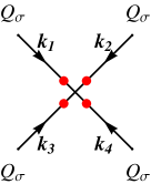
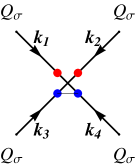
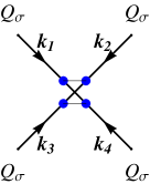
Figure 1: Diagrammatic representations of the four-point adiabatic mode self-interaction vertices. A “red dot” denotes derivative with respect to comoving time $\eta$. A blue dot denotes derivative with respect to spatial coordinates, or in Fourier space the spatial momentum. A line between two blue dots denotes “scalar-product”.

And it is easy to read the corresponding contributions according to the Feynman-diagram-like representations in fig.1:

$$\left\langle Q_{\sigma}Q_{\sigma}Q_{\sigma}Q_{\sigma}\right\rangle_{1} \equiv(2\pi)^{3}\delta^{3}(\bm{k}_{1234})\left(-2\,\Re\right)\left[24\,\Gamma_{\sigma}\,i\int_{-\infty}^{\eta_{\ast}}d\eta^{\prime}\,\frac{\textrm{d}}{\textrm{d}\eta}G_{k_{1}}(\eta_{\ast},\eta)\frac{\textrm{d}}{\textrm{d}\eta}G_{k_{2}}(\eta_{\ast},\eta)\frac{\textrm{d}}{\textrm{d}\eta}G_{k_{3}}(\eta_{\ast},\eta)\frac{\textrm{d}}{\textrm{d}\eta}G_{k_{4}}(\eta_{\ast},\eta)\right]$$ (66)

$$=(2\pi)^{3}\delta^{3}(\bm{k}_{1234})\Gamma_{\sigma}\left(-\frac{72H^{8}}{c_{a}\prod_{i}k_{i}^{3}}\right)\frac{\prod_{i}k_{i}^{2}}{K^{5}}\,,$$

where we define $K\equiv k_{1}+k_{2}+k_{3}+k_{4}$ for short.

$$\quad\;\left\langle Q_{\sigma}Q_{\sigma}Q_{\sigma}Q_{\sigma}\right\rangle_{2}$$ (67)

$$\equiv(2\pi)^{3}\delta^{3}(\bm{k}_{1234})\left(-2\,\Re\right)\left[4\,\Theta_{\sigma}\,\left(-\bm{k}_{3}\cdot\bm{k}_{4}\right)i\int_{-\infty}^{\eta_{\ast}}d\eta^{\prime}\,\frac{\textrm{d}}{\textrm{d}\eta}G_{k_{1}}(\eta_{\ast},\eta)\frac{\textrm{d}}{\textrm{d}\eta}G_{k_{2}}(\eta_{\ast},\eta)G_{k_{3}}(\eta_{\ast},\eta)G_{k_{4}}(\eta_{\ast},\eta)+\textrm{5perms }\right]$$

$$=(2\pi)^{3}\delta^{3}(\bm{k}_{1234})\Theta_{\sigma}\left(\frac{H^{8}}{c_{a}^{3}\prod_{i}k_{i}^{3}}\right)\left[\left(-\bm{k}_{3}\cdot\bm{k}_{4}\right)\frac{k_{1}^{2}k_{2}^{2}}{K^{3}}\left(1+12\frac{k_{3}k_{4}}{K^{2}}+3\frac{k_{3}+k_{4}}{K}\right)+\textrm{5perms}\right]\,,$$

where “5 perms” denotes other 5 possibilities of choosing two out of the four momenta $\bm{k}_{1}\cdots\bm{k}_{4}$ as scalar-products.

$$\quad\;\left\langle Q_{\sigma}Q_{\sigma}Q_{\sigma}Q_{\sigma}\right\rangle_{3}$$ (68)

$$\equiv(2\pi)^{3}\delta^{3}(\bm{k}_{1234})\left(-2\,\Re\right)\left[8\left(\bm{k}_{1}\cdot\bm{k}_{2}\right)\left(\bm{k}_{3}\cdot\bm{k}_{4}\right)\,\Omega_{\sigma}\,i\int_{-\infty}^{\eta_{\ast}}d\eta^{\prime}\,G_{k_{1}}(\eta_{\ast},\eta)G_{k_{2}}(\eta_{\ast},\eta)G_{k_{3}}(\eta_{\ast},\eta)G_{k_{4}}(\eta_{\ast},\eta)+2\textrm{perms}\right]$$

$$=(2\pi)^{3}\delta^{3}(\bm{k}_{1234})\Omega_{\sigma}\left(\frac{-2H^{8}}{c_{a}^{5}\prod_{i}k_{i}^{3}}\right)\left[\frac{\left(\bm{k}_{1}\cdot\bm{k}_{2}\right)\left(\bm{k}_{3}\cdot\bm{k}_{4}\right)}{K}\left(1+12\frac{\prod_{i}k_{i}}{K^{4}}+\frac{\prod_{i<j}k_{i}k_{j}}{K^{2}}+3\frac{\prod_{i}k_{i}}{K^{3}}\left(\sum_{i}\frac{1}{k_{i}}\right)\right)+2\textrm{perms}\right]\,,$$

where the other 2 permutations are combinations correspond to scalar-products $\left(\bm{k}_{1}\cdot\bm{k}_{3}\right)\left(\bm{k}_{2}\cdot\bm{k}_{4}\right)$ and $\left(\bm{k}_{1}\cdot\bm{k}_{4}\right)\left(\bm{k}_{2}\cdot\bm{k}_{3}\right)$.

It will prove convenient to define three fundamental shape functions:

$${}A_{1}(k_{1},k_{2};k_{3},k_{4}) \equiv\frac{\prod_{i}k_{i}^{2}}{K^{5}}\,,$$ (69)

$$A_{2}(k_{1},k_{2};\bm{k}_{3},\bm{k}_{4}) \equiv\left(-\bm{k}_{3}\cdot\bm{k}_{4}\right)\frac{k_{1}^{2}k_{2}^{2}}{K^{3}}\left(1+12\frac{k_{3}k_{4}}{K^{2}}+3\frac{k_{3}+k_{4}}{K}\right)\,,$$

$$A_{3}(\bm{k}_{1},\bm{k}_{2};\bm{k}_{3},\bm{k}_{4}) \equiv\frac{\left(\bm{k}_{1}\cdot\bm{k}_{2}\right)\left(\bm{k}_{3}\cdot\bm{k}_{4}\right)}{K}\left[1+12\frac{\prod_{i}^{4}k_{i}}{K^{4}}+\frac{\prod_{i<j}k_{i}k_{j}}{K^{2}}+3\frac{\prod_{i}^{4}k_{i}\left(\sum_{i}\frac{1}{k_{i}}\right)}{K^{3}}\right]\,.$$

It is useful to note two properties of these shape functions:

• permutation symmetries:
  $A_{1}(k_{1},k_{2};k_{3},k_{4})$ is completely symmetric with respect to the four momentum $k_{1}$, $k_{2}$, $k_{3}$ and $k_{4}$. $A_{2}(k_{1},k_{2};\bm{k}_{3},\bm{k}_{4})$ is symmetric under permutations $k_{1}\leftrightarrow k_{2}$ and $\bm{k}_{3}\leftrightarrow\bm{k}_{4}$. Similarly, $A_{3}(\bm{k}_{1},\bm{k}_{2};\bm{k}_{3},\bm{k}_{4})$ is symmetric under permutations of $\bm{k}_{1}\leftrightarrow\bm{k}_{2}$, $\bm{k}_{3}\leftrightarrow\bm{k}_{4}$ and $\left(\bm{k}_{1},\bm{k}_{2}\right)\leftrightarrow\left(\bm{k}_{3},\bm{k}_{4}\right)$.

• scaling properties:
  

  $$A_{1}\left(\lambda k_{1},\lambda k_{2};\lambda k_{3},\lambda k_{4}\right)=\lambda^{3}{A}_{1}\left(k_{1},k_{2},k_{3},k_{4}\right)\,,$$ (70)

  $${A}_{2}\left(\lambda k_{1},\lambda k_{2};\lambda\bm{k}_{3},\lambda\bm{k}_{4}\right)=\lambda^{3}{A}_{2}\left(k_{1},k_{2},\bm{k}_{3},\bm{k}_{4}\right)\,,$$

  $${A}_{3}\left(\lambda\bm{k}_{1},\lambda\bm{k}_{2};\lambda\bm{k}_{3},\lambda\bm{k}_{4}\right)=\lambda^{3}{A}_{3}\left(\bm{k}_{1},\bm{k}_{2},\bm{k}_{3},\bm{k}_{4}\right)\,.$$

  In other words, $A_{i}$’s have momentum dimension as $k^{3}$: $[A_{i}]=[k^{3}]$.

In terms of these three shape functions, we can write

$${}\left\langle Q_{\sigma}Q_{\sigma}Q_{\sigma}Q_{\sigma}\right\rangle_{1} =(2\pi)^{3}\delta^{3}(\bm{k}_{1234})\Gamma_{\sigma}\left(-\frac{72H^{8}}{c_{a}\prod_{i}k_{i}^{3}}\right){A}_{1}(k_{1},k_{2};k_{3},k_{4})$$ (71)

$$\equiv(2\pi)^{11}\delta^{3}(\bm{k}_{1234})\frac{\mathcal{P}_{\sigma\ast}^{4}}{\prod_{i}k_{i}^{3}}\left(-72\Gamma_{\sigma}\right){A}_{1}\left(c_{\textrm{a}}k_{1},c_{\textrm{a}}k_{2};c_{\textrm{a}}k_{3},c_{\textrm{a}}k_{4}\right)\,,$$

where we have used the scaling property ${A}_{1}\left(c_{\textrm{a}}k_{1},c_{\textrm{a}}k_{2},c_{\textrm{a}}k_{3},c_{\textrm{a}}k_{4}\right)=c_{\textrm{a}}^{3}{A}_{1}\left(k_{1},k_{2},k_{3},k_{4}\right)$. It will prove convenient to use the “sound speed dependent” (in the later we denote “$c_{s}$-dependent” for short) shape functions ${A}_{1}\left(c_{\textrm{a}}k_{1},c_{\textrm{a}}k_{2},c_{\textrm{a}}k_{3},c_{\textrm{a}}k_{4}\right)$, especially when the adiabatic mode and entropy mode have different sound speeds: $c_{\textrm{a}}\neq c_{\textrm{e}}$. Using the “$c_{s}$-dependent shape functions” not only makes the expressions simpler and more symmetric but also make the physical picture clear.

Similarly, we have

$${}\left\langle Q_{\sigma}Q_{\sigma}Q_{\sigma}Q_{\sigma}\right\rangle_{2} =(2\pi)^{11}\delta^{3}(\bm{k}_{1234})\frac{\mathcal{P}_{\sigma\ast}^{4}}{\prod_{i}k_{i}^{3}}\,\Theta_{\sigma}\frac{1}{c_{\textrm{a}}^{2}}\left[{A}_{2}(c_{\textrm{a}}k_{1},c_{\textrm{a}}k_{2};c_{\textrm{a}}\bm{k}_{3},c_{\textrm{a}}\bm{k}_{4})+\textrm{5 perms}\right]$$ (72)

$$\left\langle Q_{\sigma}Q_{\sigma}Q_{\sigma}Q_{\sigma}\right\rangle_{3} =(2\pi)^{11}\delta^{3}(\bm{k}_{1234})\frac{\mathcal{P}_{\sigma\ast}^{4}}{\prod_{i}k_{i}^{3}}\,\left(-2\Omega_{\sigma}\right)\frac{1}{c_{\textrm{a}}^{4}}\left[{A}_{3}(c_{\textrm{a}}\bm{k}_{1},c_{\textrm{a}}\bm{k}_{2};c_{\textrm{a}}\bm{k}_{3},c_{\textrm{a}}\bm{k}_{4})+\textrm{2 perms}\right]\,.$$

The whole contribution from $\left\langle Q_{\sigma}Q_{\sigma}Q_{\sigma}Q_{\sigma}\right\rangle$ is given by

$$\left\langle Q_{\sigma}Q_{\sigma}Q_{\sigma}Q_{\sigma}\right\rangle=\sum_{i}^{3}\left\langle Q_{\sigma}Q_{\sigma}Q_{\sigma}Q_{\sigma}\right\rangle_{i}\,.$$ (73)

5.1.2 $\left\langle Q_{\sigma}Q_{\sigma}Q_{s}Q_{s}\right\rangle$

There are six types of adiabatic/entropy four-point cross-interaction vertices, involving two adiabatic modes and two entropy modes, as shown in fig.2.

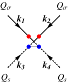
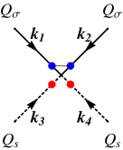
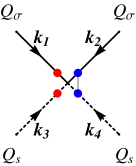
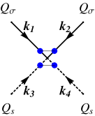
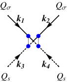
Figure 2: Diagrammatic representations of the four-point adiabatic/entropy modes cross-interaction vertices. A “red dot” denotes derivative wrt comoving time $\eta$. A blue dot donotes derivative wrt spatial coordinates, or in Fourier space the spatial momentum. A line between two blue dots denotes “scalar-product”.

$${}\left\langle Q_{\sigma}Q_{\sigma}Q_{s}Q_{s}\right\rangle_{1} \equiv(2\pi)^{3}\delta^{3}(\bm{k}_{1234})\left(-2\Re\right)\left[4\Gamma_{c}\,i\int_{-\infty}^{\eta_{\ast}}d\eta\,\frac{\textrm{d}}{\textrm{d}\eta}G_{k_{1}}(\eta_{\ast},\eta)\frac{\textrm{d}}{\textrm{d}\eta}G_{k_{2}}(\eta_{\ast},\eta)\frac{\textrm{d}}{\textrm{d}\eta}F_{k_{3}}(\eta_{\ast},\eta)\frac{\textrm{d}}{\textrm{d}\eta}F_{k_{4}}(\eta_{\ast},\eta)\right]$$ (74)

$$=(2\pi)^{3}\delta^{3}(\bm{k}_{1234})\Gamma_{c}\left(\frac{-12H^{8}}{\prod_{i}k_{i}^{3}}\right)\frac{c_{a}^{2}c_{e}^{2}\prod_{i}^{4}k_{i}^{2}}{\tilde{K}^{5}}\,.$$

where $\tilde{K}\equiv c_{\textrm{a}}\left(k_{1}+k_{2}\right)+c_{\textrm{e}}\left(k_{3}+k_{4}\right)$. In terms of the three fundamental shape functions (69), (74) can be written in a rather compact and convenient form:

$$\left\langle Q_{\sigma}Q_{\sigma}Q_{s}Q_{s}\right\rangle_{1}=(2\pi)^{11}\delta^{3}(\bm{k}_{1234})\frac{\mathcal{P}_{\sigma\ast}^{2}\mathcal{P}_{s\ast}^{2}}{\prod_{i}k_{i}^{3}}\left(-12\Gamma_{c}\right){A}_{1}\left(c_{\textrm{a}}k_{1},c_{\textrm{a}}k_{2};c_{\textrm{e}}k_{3},c_{\textrm{e}}k_{4}\right)\,,$$ (75)

where $\mathcal{P}_{\sigma}$ and $\mathcal{P}_{s}$ are the dimensionless power spectrum defined in (44). Similarly, we have (readers who are interested in their explicit expressions may refer to Appendix E)

$$\left\langle Q_{\sigma}Q_{\sigma}Q_{s}Q_{s}\right\rangle_{2} =(2\pi)^{11}\delta^{3}(\bm{k}_{1234})\frac{\mathcal{P}_{\sigma\ast}^{2}\mathcal{P}_{s\ast}^{2}}{\prod_{i}k_{i}^{3}}\,\frac{\Theta_{\sigma s}}{c_{\textrm{e}}^{2}}{A}_{2}\left(c_{\textrm{a}}k_{1},c_{\textrm{a}}k_{2};c_{\textrm{e}}\bm{k}_{3},c_{\textrm{e}}\bm{k}_{4}\right)\,,$$ (76)

$$\left\langle Q_{\sigma}Q_{\sigma}Q_{s}Q_{s}\right\rangle_{3} =(2\pi)^{11}\delta^{3}(\bm{k}_{1234})\frac{\mathcal{P}_{\sigma\ast}^{2}\mathcal{P}_{s\ast}^{2}}{\prod_{i}k_{i}^{3}}\,\frac{\Theta_{s\sigma}}{c_{\textrm{a}}^{2}}{A}_{2}\left(c_{\textrm{e}}k_{3},c_{\textrm{e}}k_{4};c_{\textrm{a}}\bm{k}_{1},c_{\textrm{a}}\bm{k}_{2}\right)\,,$$

$$\left\langle Q_{\sigma}Q_{\sigma}Q_{s}Q_{s}\right\rangle_{4} =(2\pi)^{11}\delta^{3}(\bm{k}_{1234})\frac{\mathcal{P}_{\sigma\ast}^{2}\mathcal{P}_{s\ast}^{2}}{\prod_{i}k_{i}^{3}}\,\frac{\Theta_{c}}{4\,c_{\textrm{a}}c_{\textrm{e}}}\left[{A}_{2}\left(c_{\textrm{a}}k_{1},c_{\textrm{e}}k_{3};c_{\textrm{a}}\bm{k}_{2},c_{\textrm{e}}\bm{k}_{4}\right)+{A}_{2}\left(c_{\textrm{a}}k_{1},c_{\textrm{e}}k_{4};c_{\textrm{a}}\bm{k}_{2},c_{\textrm{e}}\bm{k}_{3}\right)\right.$$

$$\qquad\qquad\qquad\qquad\qquad\qquad\qquad\left.+{A}_{2}\left(c_{\textrm{a}}k_{2},c_{\textrm{e}}k_{3};c_{\textrm{a}}\bm{k}_{1},c_{\textrm{e}}\bm{k}_{4}\right)+{A}_{2}\left(c_{\textrm{a}}k_{2},c_{\textrm{e}}k_{4};c_{\textrm{a}}\bm{k}_{1},c_{\textrm{e}}\bm{k}_{3}\right)\right]\,,$$

$$\left\langle Q_{\sigma}Q_{\sigma}Q_{s}Q_{s}\right\rangle_{5} =(2\pi)^{11}\delta^{3}(\bm{k}_{1234})\frac{\mathcal{P}_{\sigma\ast}^{2}\mathcal{P}_{s\ast}^{2}}{\prod_{i}k_{i}^{3}}\,\frac{\left(-\Omega_{\sigma s}\right)}{c_{\textrm{a}}^{2}c_{\textrm{e}}^{2}}\,{A}_{3}\left(c_{\textrm{a}}\bm{k}_{1},c_{\textrm{a}}\bm{k}_{2};c_{\textrm{e}}\bm{k}_{3},c_{\textrm{e}}\bm{k}_{4}\right)\,,$$

$$\left\langle Q_{\sigma}Q_{\sigma}Q_{s}Q_{s}\right\rangle_{6} =(2\pi)^{11}\delta^{3}(\bm{k}_{1234})\frac{\mathcal{P}_{\sigma\ast}^{2}\mathcal{P}_{s\ast}^{2}}{\prod_{i}k_{i}^{3}}\,\frac{\left(-\Omega_{c}\right)}{2c_{\textrm{a}}^{2}c_{\textrm{e}}^{2}}\left[{A}_{3}\left(c_{\textrm{a}}\bm{k}_{1},c_{\textrm{e}}\bm{k}_{3};c_{\textrm{a}}\bm{k}_{2},c_{\textrm{e}}\bm{k}_{4}\right)+{A}_{3}\left(c_{\textrm{a}}\bm{k}_{1},c_{\textrm{e}}\bm{k}_{4};c_{\textrm{a}}\bm{k}_{2},c_{\textrm{e}}\bm{k}_{3}\right)\right]\,.$$

For clarity and later convenience, we group these six contributions into three types, arising from ${A}_{1}$, ${A}_{2}$ and ${A}_{3}$ respectively. First we have,

$${}\left\langle Q_{\sigma}Q_{\sigma}Q_{s}Q_{s}\right\rangle_{{A}_{1}}\equiv\left\langle Q_{\sigma}Q_{\sigma}Q_{s}Q_{s}\right\rangle_{1}=(2\pi)^{11}\delta^{3}(\bm{k}_{1234})\frac{\mathcal{P}_{\sigma\ast}^{2}\mathcal{P}_{s\ast}^{2}}{\prod_{i}k_{i}^{3}}\left(-12\Gamma_{c}\right){A}_{1}\left(c_{\textrm{a}}k_{1},c_{\textrm{a}}k_{2};c_{\textrm{e}}k_{3},c_{\textrm{e}}k_{4}\right)\,,$$ (77)

While

$${}\left\langle Q_{\sigma}Q_{\sigma}Q_{s}Q_{s}\right\rangle_{{A}_{2}} \equiv\left\langle Q_{\sigma}Q_{\sigma}Q_{s}Q_{s}\right\rangle_{2}+\left\langle Q_{\sigma}Q_{\sigma}Q_{s}Q_{s}\right\rangle_{3}+\left\langle Q_{\sigma}Q_{\sigma}Q_{s}Q_{s}\right\rangle_{4}$$ (78)

$$=(2\pi)^{11}\delta^{3}(\bm{k}_{1234})\frac{\mathcal{P}_{\sigma\ast}^{2}\mathcal{P}_{s\ast}^{2}}{\prod_{i}k_{i}^{3}}\,\left\{\frac{\Theta_{\sigma s}}{c_{\textrm{e}}^{2}}{A}_{2}\left(c_{\textrm{a}}k_{1},c_{\textrm{a}}k_{2};c_{\textrm{e}}\bm{k}_{3},c_{\textrm{e}}\bm{k}_{4}\right)+\frac{\Theta_{s\sigma}}{c_{\textrm{a}}^{2}}{A}_{2}\left(c_{\textrm{e}}k_{3},c_{\textrm{e}}k_{4};c_{\textrm{a}}\bm{k}_{1},c_{\textrm{a}}\bm{k}_{2}\right)\right.$$

$$\qquad\qquad\qquad\qquad+\frac{\Theta_{c}}{4c_{\textrm{a}}c_{\textrm{e}}}\left[{A}_{2}\left(c_{\textrm{a}}k_{1},c_{\textrm{e}}k_{3};c_{\textrm{a}}\bm{k}_{2},c_{\textrm{e}}\bm{k}_{4}\right)+{A}_{2}\left(c_{\textrm{a}}k_{1},c_{\textrm{e}}k_{4};c_{\textrm{a}}\bm{k}_{2},c_{\textrm{e}}\bm{k}_{3}\right)\right.$$

$$\qquad\qquad\qquad\qquad\qquad\qquad\left.+{A}_{2}\left(c_{\textrm{a}}k_{2},c_{\textrm{e}}k_{3};c_{\textrm{a}}\bm{k}_{1},c_{\textrm{e}}\bm{k}_{4}\right)+{A}_{2}\left(c_{\textrm{a}}k_{2},c_{\textrm{e}}k_{4};c_{\textrm{a}}\bm{k}_{1},c_{\textrm{e}}\bm{k}_{3}\right)\right]\Big{\}}\,,$$

and

$${}\left\langle Q_{\sigma}Q_{\sigma}Q_{s}Q_{s}\right\rangle_{{A}_{3}} \equiv\left\langle Q_{\sigma}Q_{\sigma}Q_{s}Q_{s}\right\rangle_{5}+\left\langle Q_{\sigma}Q_{\sigma}Q_{s}Q_{s}\right\rangle_{6}$$ (79)

$$=(2\pi)^{11}\delta^{3}(\bm{k}_{1234})\frac{\mathcal{P}_{\sigma\ast}^{2}\mathcal{P}_{s\ast}^{2}}{\prod_{i}k_{i}^{3}}\,\left\{\frac{\left(-\Omega_{\sigma s}\right)}{c_{\textrm{a}}^{2}c_{\textrm{e}}^{2}}\,{A}_{3}\left(c_{\textrm{a}}\bm{k}_{1},c_{\textrm{a}}\bm{k}_{2};c_{\textrm{e}}\bm{k}_{3},c_{\textrm{e}}\bm{k}_{4}\right)\right.$$

$$\qquad\qquad\qquad\qquad\left.+\frac{\left(-\Omega_{c}\right)}{2c_{\textrm{a}}^{2}c_{\textrm{e}}^{2}}\left[\mathcal{A}_{3}\left(c_{\textrm{a}}\bm{k}_{1},c_{\textrm{e}}\bm{k}_{3};c_{\textrm{a}}\bm{k}_{2},c_{\textrm{e}}\bm{k}_{4}\right)+{A}_{3}\left(c_{\textrm{a}}\bm{k}_{1},c_{\textrm{e}}\bm{k}_{4};c_{\textrm{a}}\bm{k}_{2},c_{\textrm{e}}\bm{k}_{3}\right)\right]\right\}\,.$$

The whole contribution from $\left\langle Q_{\sigma}Q_{\sigma}Q_{s}Q_{s}\right\rangle$ is given by

$$\left\langle Q_{\sigma}(\bm{k}_{1},\eta_{\ast})Q_{\sigma}(\bm{k}_{2},\eta_{\ast})Q_{s}(\bm{k}_{3},\eta_{\ast})Q_{s}(\bm{k}_{4},\eta_{\ast})\right\rangle\equiv\left\langle Q_{\sigma}Q_{\sigma}Q_{s}Q_{s}\right\rangle_{{A}_{1}}+\left\langle Q_{\sigma}Q_{\sigma}Q_{s}Q_{s}\right\rangle_{{A}_{2}}+\left\langle Q_{\sigma}Q_{\sigma}Q_{s}Q_{s}\right\rangle_{{A}_{3}}\,.$$ (80)

5.1.3 $\left\langle Q_{s}Q_{s}Q_{s}Q_{s}\right\rangle$

There are also three types of $Q_{s}$ self-interaction four-point vertices, as shown in fig.3. $\left\langle Q_{s}Q_{s}Q_{s}Q_{s}\right\rangle$ are easily obtained by simply changing the corresponding “effective couplings” and $\mathcal{P}_{\sigma}\leftrightarrow\mathcal{P}_{s}$ and $c_{\textrm{a}}\leftrightarrow c_{\textrm{e}}$ in (71)-(72):

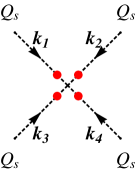
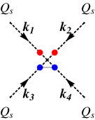
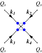
Figure 3: Diagrammatic representations of the four-point entropy mode self-interaction vertices. A “red dot” denotes derivative wrt comoving time $\eta$. A blut dot donotes derivative wrt spatial coordinates, or in fourier space the spatial momentum. A line between two blue dots denotes “scalar-product”.

$${}\left\langle Q_{s}Q_{s}Q_{s}Q_{s}\right\rangle_{1} =(2\pi)^{11}\delta^{3}(\bm{k}_{1234})\frac{\mathcal{P}_{s\ast}^{4}}{\prod_{i}^{4}k_{i}^{3}}\left(-72\Gamma_{s}\right){A}_{1}\left(c_{\textrm{e}}k_{1},c_{\textrm{e}}k_{2},c_{\textrm{e}}k_{3},c_{\textrm{e}}k_{4}\right)\,,$$ (81)

$$\left\langle Q_{s}Q_{s}Q_{s}Q_{s}\right\rangle_{2} =(2\pi)^{11}\delta^{3}(\bm{k}_{1234})\frac{\mathcal{P}_{s\ast}^{4}}{\prod_{i}^{4}k_{i}^{3}}\,\Theta_{s}\frac{1}{c_{\textrm{e}}^{2}}\left[{A}_{2}(c_{\textrm{e}}k_{1},c_{\textrm{e}}k_{2};c_{\textrm{e}}\bm{k}_{3},c_{\textrm{e}}\bm{k}_{4})+\textrm{5 perms}\right]$$

$$\left\langle Q_{s}Q_{s}Q_{s}Q_{s}\right\rangle_{3} =(2\pi)^{11}\delta^{3}(\bm{k}_{1234})\frac{\mathcal{P}_{s\ast}^{4}}{\prod_{i}^{4}k_{i}^{3}}\,\left(-2\Omega_{s}\right)\frac{1}{c_{\textrm{e}}^{4}}\left[{A}_{3}(c_{\textrm{e}}\bm{k}_{1},c_{\textrm{e}}\bm{k}_{2};c_{\textrm{e}}\bm{k}_{3},c_{\textrm{e}}\bm{k}_{4})+\textrm{2 perms}\right]\,.$$

The whole contribution from $\left\langle Q_{s}Q_{s}Q_{s}Q_{s}\right\rangle$ is given by

$$\quad\;\left\langle Q_{s}(\bm{k}_{1},\eta_{\ast})Q_{s}(\bm{k}_{2},\eta_{\ast})Q_{s}(\bm{k}_{3},\eta_{\ast})Q_{s}(\bm{k}_{4},\eta_{\ast})\right\rangle=\sum_{i}^{3}\left\langle Q_{s}Q_{s}Q_{s}Q_{s}\right\rangle_{i}\,.$$ (82)

5.2 Four-point Function of the Curvature Perturbation $\left\langle\mathcal{R}^{4}\right\rangle$

As we have addressed before, the scalar-field perturbations $Q_{\sigma}$ and $Q_{s}$ themselves are not directly observable. What we are eventually interested in is the curvature perturbation $\mathcal{R}$. As has been investigated in [57, 58, 62], this can be achieved by writing

$$\mathcal{R} \approx\mathcal{R}_{\ast}+T_{\mathcal{R}\mathcal{S}}\mathcal{S}_{\ast}=\left(\frac{H}{\dot{\sigma}}\right)_{\ast}Q_{\sigma\ast}+T_{\mathcal{R}\mathcal{S}}\left(\frac{H}{\dot{\sigma}}\right)_{\ast}Q_{s\ast}$$ (83)

$$\equiv\mathcal{N}_{\sigma}Q_{\sigma\ast}+\mathcal{N}_{s}Q_{s\ast}\,.$$

Note that $\mathcal{N}_{s}\equiv T_{\mathcal{R}\mathcal{S}}\mathcal{N}_{\sigma}$ is in general time-dependent. The four-point correlation function for comoving curvature perturbation $\mathcal{R}$ is given by

$$\quad\;\left\langle\mathcal{R}(\bm{k}_{1})\mathcal{R}(\bm{k}_{3})\mathcal{R}(\bm{k}_{2})\mathcal{R}(\bm{k}_{4})\right\rangle$$ (84)

$$=\mathcal{N}_{\sigma}^{4}\left\langle Q_{\sigma}(\bm{k}_{1})Q_{\sigma}(\bm{k}_{2})Q_{\sigma}(\bm{k}_{3})Q_{\sigma}(\bm{k}_{4})\right\rangle_{\ast}+\mathcal{N}_{\sigma}^{2}\mathcal{N}_{s}^{2}\left[\left\langle Q_{\sigma}(\bm{k}_{1})Q_{\sigma}(\bm{k}_{2})Q_{s}(\bm{k}_{3})Q_{s}(\bm{k}_{4})\right\rangle_{\ast}+\textrm{5 perms}\right]$$

$$\qquad\qquad+\mathcal{N}_{s}^{4}\left\langle Q_{s}(\bm{k}_{1})Q_{s}(\bm{k}_{2})Q_{s}(\bm{k}_{3})Q_{s}(\bm{k}_{4})\right\rangle_{\ast}\,,$$

where “5 perms” denotes other 5 possibilities of choosing two momenta for $Q_{\sigma}$ and two momenta for $Q_{s}$ out of the four momenta. In deriving (LABEL:4R_original), we have used the assumption that there is no cross-correlation between adiabatic and entropy modes around horizon-crossing, i.e. $\left\langle Q_{\sigma}Q_{s}\right\rangle_{\ast}\equiv 0$. This is indeed the case if we use the second-order perturbation action (29) as our starting point of canonical quantization.

It is also convenient to group the whole contributions to $\left\langle\mathcal{R}^{4}\right\rangle$ (LABEL:4R_original) into three types, which correspond to three different physical origins or more precisely three different types of four-point interaction vertices. From (71), (77) and (81), we have

$${}\left\langle\mathcal{R}^{4}\right\rangle_{1} \equiv(2\pi)^{11}\delta^{3}(\bm{k}_{1234})\frac{1}{\prod_{i}k_{i}^{3}}\left\{\mathcal{N}_{\sigma}^{4}\mathcal{P}_{\sigma\ast}^{4}\left(-12\Gamma_{\sigma}\right){A}_{1}\left(c_{\textrm{a}}k_{1},c_{\textrm{a}}k_{2};c_{\textrm{a}}k_{3},c_{\textrm{a}}k_{4}\right)\right.$$ (85)

$$\qquad\qquad+\mathcal{N}_{\sigma}^{2}\mathcal{N}_{s}^{2}\mathcal{P}_{\sigma\ast}^{2}\mathcal{P}_{s\ast}^{2}\,\left(-12\Gamma_{c}\right){A}_{1}\left(c_{\textrm{a}}k_{1},c_{\textrm{a}}k_{2};c_{\textrm{e}}k_{3},c_{\textrm{e}}k_{4}\right)$$

$$\qquad\qquad\left.+\mathcal{N}_{s}^{4}\mathcal{P}_{s\ast}^{4}\,\left(-12\Gamma_{s}\right){A}_{1}\left(c_{\textrm{e}}k_{1},c_{\textrm{e}}k_{2},c_{\textrm{e}}k_{3},c_{\textrm{e}}k_{4}\right)+\textrm{5 perms}\right\}$$

$$=(2\pi)^{11}\delta^{3}(\bm{k}_{1234})\frac{-12\mathcal{N}_{\sigma}^{4}\mathcal{P}_{\sigma\ast}^{4}}{\prod_{i}k_{i}^{3}}\bigg{\{}\Gamma_{\sigma}\,{A}_{1}\left(c_{\textrm{a}}k_{1},c_{\textrm{a}}k_{2};c_{\textrm{a}}k_{3},c_{\textrm{a}}k_{4}\right)$$

$$\qquad\qquad+\left(T_{\mathcal{R}\mathcal{S}}\frac{c_{\textrm{a}}}{c_{\textrm{e}}}\right)^{2}\,\Gamma_{c}\,{A}_{1}\left(c_{\textrm{a}}k_{1},c_{\textrm{a}}k_{2};c_{\textrm{e}}k_{3},c_{\textrm{e}}k_{4}\right)$$

$$\qquad\qquad\left.+\left(T_{\mathcal{R}\mathcal{S}}\frac{c_{\textrm{a}}}{c_{\textrm{e}}}\right)^{4}\,\Gamma_{s}\,{A}_{1}\left(c_{\textrm{e}}k_{1},c_{\textrm{e}}k_{2},c_{\textrm{e}}k_{3},c_{\textrm{e}}k_{4}\right)+\textrm{5 perms}\right\}\,,$$

where we have used $\mathcal{N}_{s}\equiv T_{\mathcal{R}\mathcal{S}}\mathcal{N}_{\sigma}$ and the fact that $\mathcal{P}_{s}/\mathcal{P}_{\sigma}=c_{\textrm{a}}/c_{\textrm{e}}$. “5 perms” denotes other 5 possibilities of choosing two out from the four momenta $k_{1},\cdots,k_{4}$ as the first two arguments of ${A}_{1}$ and the other two momenta as the last two arguments of ${A}_{1}$(obviously the differences only arise in ${A}_{1}\left(c_{\textrm{a}}k_{1},c_{\textrm{a}}k_{2};c_{\textrm{e}}k_{3},c_{\textrm{e}}k_{4}\right)$). Similarly, we have

$${}\left\langle\mathcal{R}^{4}\right\rangle_{2} =(2\pi)^{11}\delta^{3}(\bm{k}_{1234})\frac{\mathcal{N}_{\sigma}^{4}\mathcal{P}_{\sigma\ast}^{4}}{\prod_{i}k_{i}^{3}}\left\{\frac{\Theta_{\sigma}}{c_{\textrm{a}}^{2}}{A}_{2}(c_{\textrm{a}}k_{1},c_{\textrm{a}}k_{2};c_{\textrm{a}}\bm{k}_{3},c_{\textrm{a}}\bm{k}_{4})\right.$$ (86)

$$\qquad\qquad+\left(T_{\mathcal{R}\mathcal{S}}\frac{c_{\textrm{a}}}{c_{\textrm{e}}}\right)^{2}\left[\frac{\Theta_{\sigma s}}{c_{\textrm{e}}^{2}}{A}_{2}\left(c_{\textrm{a}}k_{1},c_{\textrm{a}}k_{2};c_{\textrm{e}}\bm{k}_{3},c_{\textrm{e}}\bm{k}_{4}\right)+\frac{\Theta_{s\sigma}}{c_{\textrm{a}}^{2}}{A}_{2}\left(c_{\textrm{e}}k_{3},c_{\textrm{e}}k_{4};c_{\textrm{a}}\bm{k}_{1},c_{\textrm{a}}\bm{k}_{2}\right)\right.$$

$$\qquad\qquad\qquad\qquad+\frac{\Theta_{c}}{4c_{\textrm{a}}c_{\textrm{e}}}\left[{A}_{2}\left(c_{\textrm{a}}k_{1},c_{\textrm{e}}k_{3};c_{\textrm{a}}\bm{k}_{2},c_{\textrm{e}}\bm{k}_{4}\right)+{A}_{2}\left(c_{\textrm{a}}k_{1},c_{\textrm{e}}k_{4};c_{\textrm{a}}\bm{k}_{2},c_{\textrm{e}}\bm{k}_{3}\right)\right.$$

$$\qquad\qquad\qquad\qquad\qquad\qquad\left.+{A}_{2}\left(c_{\textrm{a}}k_{2},c_{\textrm{e}}k_{3};c_{\textrm{a}}\bm{k}_{1},c_{\textrm{e}}\bm{k}_{4}\right)+{A}_{2}\left(c_{\textrm{a}}k_{2},c_{\textrm{e}}k_{4};c_{\textrm{a}}\bm{k}_{1},c_{\textrm{e}}\bm{k}_{3}\right)\right]\bigg{]}$$

$$\qquad\qquad+\left(T_{\mathcal{R}\mathcal{S}}\frac{c_{\textrm{a}}}{c_{\textrm{e}}}\right)^{4}\frac{\Theta_{s}}{c_{\textrm{e}}^{2}}{A}_{2}(c_{\textrm{e}}k_{1},c_{\textrm{e}}k_{2};c_{\textrm{e}}\bm{k}_{3},c_{\textrm{e}}\bm{k}_{4})+\textrm{5 perms}\bigg{\}}\,,$$

and

$${}\left\langle\mathcal{R}^{4}\right\rangle_{3} =(2\pi)^{11}\delta^{3}(\bm{k}_{1234})\frac{\mathcal{N}_{\sigma}^{4}\mathcal{P}_{\sigma\ast}^{4}}{\prod_{i}k_{i}^{3}}\left\{\frac{\left(-\Omega_{\sigma}\right)}{c_{\textrm{a}}^{4}}{A}_{3}(c_{\textrm{a}}\bm{k}_{1},c_{\textrm{a}}\bm{k}_{2};c_{\textrm{a}}\bm{k}_{3},c_{\textrm{a}}\bm{k}_{4})\right.$$ (87)

$$\qquad\qquad\qquad\qquad+\left(T_{\mathcal{R}\mathcal{S}}\frac{c_{\textrm{a}}}{c_{\textrm{e}}}\right)^{2}\left[\frac{\left(-\Omega_{\sigma s}\right)}{c_{\textrm{a}}^{2}c_{\textrm{e}}^{2}}\,{A}_{3}\left(c_{\textrm{a}}\bm{k}_{1},c_{\textrm{a}}\bm{k}_{2};c_{\textrm{e}}\bm{k}_{3},c_{\textrm{e}}\bm{k}_{4}\right)\right.$$

$$\qquad\qquad\qquad\qquad\qquad\qquad\left.+\frac{\left(-\Omega_{c}\right)}{2c_{\textrm{a}}^{2}c_{\textrm{e}}^{2}}\left[{A}_{3}\left(c_{\textrm{a}}\bm{k}_{1},c_{\textrm{e}}\bm{k}_{3};c_{\textrm{a}}\bm{k}_{2},c_{\textrm{e}}\bm{k}_{4}\right)+{A}_{3}\left(c_{\textrm{a}}\bm{k}_{1},c_{\textrm{e}}\bm{k}_{4};c_{\textrm{a}}\bm{k}_{2},c_{\textrm{e}}\bm{k}_{3}\right)\right]\right]$$

$$\qquad\qquad\qquad\qquad\left.+\left(T_{\mathcal{R}\mathcal{S}}\frac{c_{\textrm{a}}}{c_{\textrm{e}}}\right)^{4}\frac{\left(-\Omega_{s}\right)}{c_{\textrm{e}}^{4}}{A}_{3}(c_{\textrm{e}}\bm{k}_{1},c_{\textrm{e}}\bm{k}_{2};c_{\textrm{e}}\bm{k}_{3},c_{\textrm{e}}\bm{k}_{4})+\textrm{5 perms}\right\}\,.$$

It is convenient to define three new shape functions, which can be viewed as the generalizations of the three fundamental shapes (69).

$${}\mathcal{A}_{1}\left(k_{1},k_{2},k_{3},k_{3}\right) \equiv{A}_{1}\left(c_{\textrm{a}}k_{1},c_{\textrm{a}}k_{2};c_{\textrm{a}}k_{3},c_{\textrm{a}}k_{4}\right)+\left(T_{\mathcal{R}\mathcal{S}}\frac{c_{\textrm{a}}}{c_{\textrm{e}}}\right)^{2}\,\frac{\Gamma_{c}}{\Gamma_{\sigma}}\,{A}_{1}\left(c_{\textrm{a}}k_{1},c_{\textrm{a}}k_{2};c_{\textrm{e}}k_{3},c_{\textrm{e}}k_{4}\right)$$ (88)

$$\qquad\qquad+\left(T_{\mathcal{R}\mathcal{S}}\frac{c_{\textrm{a}}}{c_{\textrm{e}}}\right)^{4}\,\frac{\Gamma_{s}}{\Gamma_{\sigma}}\,{A}_{1}\left(c_{\textrm{e}}k_{1},c_{\textrm{e}}k_{2},c_{\textrm{e}}k_{3},c_{\textrm{e}}k_{4}\right)+\textrm{5 perms}\,,$$

$${}\mathcal{A}_{2}(\bm{k}_{1},\bm{k}_{2};\bm{k}_{3},\bm{k}_{4}) \equiv\frac{1}{c_{\textrm{a}}^{2}}{A}_{2}(c_{\textrm{a}}k_{1},c_{\textrm{a}}k_{2};c_{\textrm{a}}\bm{k}_{3},c_{\textrm{a}}\bm{k}_{4})$$ (89)

$$\qquad\qquad+\left(T_{\mathcal{R}\mathcal{S}}\frac{c_{\textrm{a}}}{c_{\textrm{e}}}\right)^{2}\frac{1}{\Theta_{\sigma}}\left[\frac{\Theta_{\sigma s}}{c_{\textrm{e}}^{2}}{A}_{2}\left(c_{\textrm{a}}k_{1},c_{\textrm{a}}k_{2};c_{\textrm{e}}\bm{k}_{3},c_{\textrm{e}}\bm{k}_{4}\right)+\frac{\Theta_{s\sigma}}{c_{\textrm{a}}^{2}}{A}_{2}\left(c_{\textrm{e}}k_{3},c_{\textrm{e}}k_{4};c_{\textrm{a}}\bm{k}_{1},c_{\textrm{a}}\bm{k}_{2}\right)\right.$$

$$\qquad\qquad\qquad\qquad+\frac{\Theta_{c}}{4c_{\textrm{a}}c_{\textrm{e}}}\left[{A}_{2}\left(c_{\textrm{a}}k_{1},c_{\textrm{e}}k_{3};c_{\textrm{a}}\bm{k}_{2},c_{\textrm{e}}\bm{k}_{4}\right)+{A}_{2}\left(c_{\textrm{a}}k_{1},c_{\textrm{e}}k_{4};c_{\textrm{a}}\bm{k}_{2},c_{\textrm{e}}\bm{k}_{3}\right)\right.$$

$$\qquad\qquad\qquad\qquad\qquad\qquad\left.+{A}_{2}\left(c_{\textrm{a}}k_{2},c_{\textrm{e}}k_{3};c_{\textrm{a}}\bm{k}_{1},c_{\textrm{e}}\bm{k}_{4}\right)+{A}_{2}\left(c_{\textrm{a}}k_{2},c_{\textrm{e}}k_{4};c_{\textrm{a}}\bm{k}_{1},c_{\textrm{e}}\bm{k}_{3}\right)\right]\bigg{]}$$

$$\qquad\qquad+\left(T_{\mathcal{R}\mathcal{S}}\frac{c_{\textrm{a}}}{c_{\textrm{e}}}\right)^{4}\frac{\Theta_{s}}{\Theta_{\sigma}c_{\textrm{e}}^{2}}{A}_{2}(c_{\textrm{e}}k_{1},c_{\textrm{e}}k_{2};c_{\textrm{e}}\bm{k}_{3},c_{\textrm{e}}\bm{k}_{4})+\textrm{5 perms}\,,$$

and

$${}\mathcal{A}_{3}(\bm{k}_{1},\bm{k}_{2};\bm{k}_{3},\bm{k}_{4}) \equiv\frac{1}{c_{\textrm{a}}^{4}}{A}_{3}(c_{\textrm{a}}\bm{k}_{1},c_{\textrm{a}}\bm{k}_{2};c_{\textrm{a}}\bm{k}_{3},c_{\textrm{a}}\bm{k}_{4})$$ (90)

$$\qquad\qquad+\left(T_{\mathcal{R}\mathcal{S}}\frac{c_{\textrm{a}}}{c_{\textrm{e}}}\right)^{2}\frac{1}{\Omega_{\sigma}}\left[\frac{\Omega_{\sigma s}}{c_{\textrm{a}}^{2}c_{\textrm{e}}^{2}}\,{A}_{3}\left(c_{\textrm{a}}\bm{k}_{1},c_{\textrm{a}}\bm{k}_{2};c_{\textrm{e}}\bm{k}_{3},c_{\textrm{e}}\bm{k}_{4}\right)\right.$$

$$\qquad\qquad\qquad\qquad\left.+\frac{\Omega_{c}}{2c_{\textrm{a}}^{2}c_{\textrm{e}}^{2}}\left[{A}_{3}\left(c_{\textrm{a}}\bm{k}_{1},c_{\textrm{e}}\bm{k}_{3};c_{\textrm{a}}\bm{k}_{2},c_{\textrm{e}}\bm{k}_{4}\right)+{A}_{3}\left(c_{\textrm{a}}\bm{k}_{1},c_{\textrm{e}}\bm{k}_{4};c_{\textrm{a}}\bm{k}_{2},c_{\textrm{e}}\bm{k}_{3}\right)\right]\right]$$

$$\qquad\qquad+\left(T_{\mathcal{R}\mathcal{S}}\frac{c_{\textrm{a}}}{c_{\textrm{e}}}\right)^{4}\frac{\Omega_{s}}{\Omega_{\sigma}c_{\textrm{e}}^{4}}{A}_{3}(c_{\textrm{e}}\bm{k}_{1},c_{\textrm{e}}\bm{k}_{2};c_{\textrm{e}}\bm{k}_{3},c_{\textrm{e}}\bm{k}_{4})+\textrm{5 perms}\,.$$

Note that $\mathcal{A}_{i}$ also depend on parameters $c_{\textrm{a}}$, $c_{\textrm{e}}$, $\lambda$, $\Pi$ and $T_{\mathcal{R}\mathcal{S}}$. In multi-field models, these parameters enter the definition of the shapes. This is essentially different from that in single-field models, we can always abstract shape functions, which are functions of momenta only. In terms of these three “generalized shape functions” (88)-(90), the four-point correlation function for comoving curvature perturbation $\mathcal{R}$ can be recast into a rather convenient form:

$${}\left\langle\mathcal{R}(\bm{k}_{1})\mathcal{R}(\bm{k}_{2})\mathcal{R}(\bm{k}_{3})\mathcal{R}(\bm{k}_{4})\right\rangle=(2\pi)^{11}\delta^{3}(\bm{k}_{1234})\frac{\mathcal{N}_{\sigma}^{4}\mathcal{P}_{\sigma\ast}^{4}}{\prod_{i}k_{i}^{3}}\left[-12\Gamma_{\sigma}\mathcal{A}_{1}+\Theta_{\sigma}\mathcal{A}_{2}-\Omega_{\sigma}\mathcal{A}_{3}\right]\,.$$ (91)

5.2.1 Trispectrum of $\mathcal{R}$

In practice, it is convenient to define a so-called trispectrum for $\mathcal{R}$:

$${}\left\langle\mathcal{R}(\bm{k}_{1})\mathcal{R}(\bm{k}_{2})\mathcal{R}(\bm{k}_{3})\mathcal{R}(\bm{k}_{4})\right\rangle\equiv(2\pi)^{3}\delta^{3}(\bm{k}_{1234})T_{\mathcal{R}}(\bm{k}_{1},\bm{k}_{2},\bm{k}_{3},\bm{k}_{4})\,.$$ (92)

From (91) we have

$${}T_{\mathcal{R}}(\bm{k}_{1},\bm{k}_{2},\bm{k}_{3},\bm{k}_{4}) =\frac{H^{8}}{4\epsilon^{2}c_{\textrm{a}}^{4}}\frac{1}{\prod_{i}k_{i}^{3}}\left(-12\Gamma_{\sigma}\mathcal{A}_{1}+\Theta_{\sigma}\mathcal{A}_{2}-\Omega_{\sigma}\mathcal{A}_{3}\right)$$ (93)

$$=(2\pi)^{6}\mathcal{P}_{\mathcal{R}\ast}^{3}\frac{2H^{2}\epsilon}{c_{\textrm{a}}\prod_{i}k_{i}^{3}}\left(-12\Gamma_{\sigma}\mathcal{A}_{1}+\Theta_{\sigma}\mathcal{A}_{2}-\Omega_{\sigma}\mathcal{A}_{3}\right)\,,$$

where we have used $\mathcal{N}_{\sigma}^{2}=1/2\epsilon$ and $\mathcal{P}_{\sigma\ast}=\frac{1}{c_{\textrm{a}}}\left(\frac{H}{2\pi}\right)^{2}$. At this point, it is useful to note the dimensions of various quantities:

• $[\Gamma_{\sigma}]=[\Theta_{\sigma}]=[\Omega_{\sigma}]=[1/H^{2}]$,

• $[\mathcal{A}_{1}]=[\mathcal{A}_{2}]=[\mathcal{A}_{3}]=[k^{3}]$,

• thus, the trispectrum has dimension as $[T_{\mathcal{R}}]=[H^{6}/k^{9}]$. (Recall that the power spectrum has dimension $[P_{\mathcal{R}}]=[H^{2}/k^{3}]$, and the bispectrum has dimension $[B_{\mathcal{R}}]=[H^{4}/k^{6}]$.)

To end this section, we would like to make several comments.

• In this work we investigate multi-field models with Lagrangian of the form (26), which are general function of two independent contractions $X=X^{I}_{I}$ and $Y=X^{I}_{J}X^{J}_{I}$. One may expect at first that the parameter space for the trispectra will become more complicated. However, as we have shown explicitly in this work, the final (leading-order) trispectrum for $\mathcal{R}$ is controlled by six “parameters”: $\epsilon$, $c_{\textrm{a}}$, $c_{\textrm{e}}$, $\lambda$, $\Pi$ and $T_{\mathcal{R}\mathcal{S}}$. Especially, the non-linear structure of $P(X,Y,\phi^{I})$ affect the final trispectrum through $c_{\textrm{a}}$, $c_{\textrm{e}}$, $\lambda$ and $\Pi$, which are specific combinations of derivative of $P$ with respect to $X$ and $Y$ (see (28) and (31)). On the other hand, this fact would make it more difficult to determine the structure of a multi-field model from observations, since the functional forms of $P$ are highly degenerate with respect to the parameter space of trispectra.

• In the limit of small speed sounds ($c_{\textrm{a}}\ll 1$, $c_{\textrm{e}}\ll 1$), at the leading-order, there are three types of “contact four-point interaction vertices” according to the “derivatives”: vertices with four temporal derivatives, vertices with two temporal derivatives and two spatial derivative, vertices with four spatial derivatives (as illustrated in e.g. Fig.1). This is exactly the same as in general single-field models, where three types of contact interaction vertices correspond to three different “$c_{s}$-independent” shape functions. However, the subtlety is that, although in multi-field case the interaction vertices can still be grouped into these three types as in single-field case, since there are more fields and more speeds of sound, parameters arising from the non-linear structure of the theory enter into the definition of shape functions, as in (88), (89) and (90). Thus, in general there is no hope to abstract pure momentum-dependent shape functions without involving $\epsilon$, $c_{\textrm{a}}$, $c_{\textrm{e}}$, $\lambda$, $\Pi$ and $T_{\mathcal{R}\mathcal{S}}$, and thus the so-called shape functions in general take the form

  $$\mathcal{A}(\bm{k}_{1},\bm{k}_{2},\bm{k}_{3},\bm{k}_{4};\epsilon,c_{\textrm{a}},c_{\textrm{e}},\lambda,\Pi,T_{\mathcal{R}\mathcal{S}})\,.$$

  This fact makes the analysis of the shapes of non-Gaussianities in multi-field models much more complicated.

6 Characterizing the Trispectrum

For the power spectrum, it is easy to plot a curve for $P(k)$ which is a function of a single variable $k$. However, for higher-order correlation functions, or their fourier transformations bispectrum, trispectrum, etc, it is not easy to abstract simple quantities to characterize them. While from the point of view of comparing theories with observations, this is obviously one of the most important aspects in higher-order statistics of cosmological perturbations.

In this section, first we analyze the “parameter space” for the trispectrum or general higher-order correlation functions. Base on the discuss on “inequivalent momentum configurations”, we plot various “shape” diagrams which characterize the trispectrum on a 2-dimensional subspace of its whole parametric space. These “shape” diagrams are efficient for characterizing the trispectrum (or higher-order correlation functions) and are also convenient for visualization. In the end of this section, we map the trispectrum to real numbers, which can be seen as the analogue of non-linear parameters $\tau_{\textrm{NL}}$ and $g_{\textrm{NL}}$ in the literatures.

6.1 Parameter Space for the Trispectrum

In general, the four-point correlation function, or its Fourier transformation, the trispectrum, is a function of four 3D momenta: $T\left(\bm{k}_{1},\bm{k}_{2},\bm{k}_{3},\bm{k}_{4}\right)$. Let us first analyze the “dimension” of the parameter space of $T\left(\bm{k}_{1},\bm{k}_{2},\bm{k}_{3},\bm{k}_{4}\right)$, i.e., the number of independent degrees of freedom in order to identify a “inequivalent momentum configuration” (in other words, the dimension of “equivalent class” of momentum configurations). At first, we need 12 real numbers to specify a set of four 3D momenta $\{\bm{k}_{1},\bm{k}_{2},\bm{k}_{3},\bm{k}_{4}\}$. However, the 3D momentum conservation ($\bm{k}_{1}+\bm{k}_{2}+\bm{k}_{3}+\bm{k}_{4}=0$) eliminate 3 of them, and since the cosmological perturbation is assumed to be statistically homogeneous and isotropic, we have 3 dimensional rotation symmetry SO(3) which eliminates another 3 of them (that is, we call two momentum configurations are “equivalent” if they can be related by SO(3) transformation). Thus, the dimension of parameter space for trispectrum is 6. This argument can be generalized to arbitrary higher-order correlation functions. In general we need

$$3n-6\,,\qquad(n\geq 3)$$ (94)

real parameters to specify a momentum configuration for a $n$-point function. While case for $n=2$ is trivial, it is well-known that the power spectrum is a function of one parameter $k\equiv|\bm{k}|$. For example, the three-point function or its fourier transformation bispectrum takes the form $B(k_{1},k_{2},k_{3})$, which depends only on the modulus of three momenta, which are the nature choices of parameters for the bispectrum. In the case of trispectrum, things become much more involved, since we need 6 parameters.

• One possible choice is to choose a set of 6 parameters $\{k_{1},k_{2},k_{3},k_{4},k_{12},k_{23}\}$ with $k_{12}\equiv|\bm{k}_{1}+\bm{k}_{2}|$ and $k_{23}\equiv|\bm{k}_{2}+\bm{k}_{3}|$. A pictorial presentation is depicted in fig. 5.

  

  Figure 4: Pictorial representation of sets of six parameters $\{k_{1},k_{2},k_{3},k_{4},k_{12},k_{23}\}$ or $\{k_{1},k_{2},k_{12},\theta_{1},\theta_{2},\theta_{3}\}$ to specify an inequivalent 3D momentum configuration for trispectrum.

  

  Figure 5: Pictorial representation of a sef of five parameters $\{k_{1},k_{2},k_{3},k_{4},k_{12}\}$ to specify an inequivalent planar momentum configuration for trispectrum.

  At this point, it is useful to write down other four $k_{ij}\equiv|\bm{k}_{i}+\bm{k}_{j}|$ in terms of $\{k_{1},k_{2},k_{3},k_{4},k_{12},k_{23}\}$ for later convenience

  $${}k_{13} \equiv k_{24}=\sqrt{k_{1}^{2}+k_{2}^{2}+k_{3}^{2}+k_{4}^{2}-k_{12}^{2}-k_{23}^{2}}\,,$$ (95)

  $$k_{14} \equiv k_{23}\,,\qquad\qquad k_{34}\equiv k_{12}\,.$$

  Obviously, these six momenta cannot take all real values simultaneously. Actually they should satisfy the so-called “triangle inequalities” (remember we have (95)):

  $$k_{i}+k_{j}\geq k_{ij}\,,\qquad k_{i}+k_{ij}\geq k_{j}\,,\qquad(i,j=1,2,3,4\quad\textrm{and}\quad i\neq j)\,.$$ (96)

• Another possible parameterization is to choose three momenta and three angles: $\{k_{1},k_{2},k_{23},\theta_{1},\theta_{2},\theta_{3}\}$ (see also fig.5). Similarly, the three angles $\theta_{1},\theta_{2},\theta_{3}$ should satisfy:

  $$\theta_{i}+\theta_{j} \geq\theta_{k}\,,\qquad(i,j,k=1,2,3\,\quad\textrm{and}\quad i\neq j\neq k)\,,$$ (97)

  $$\theta_{1}+\theta_{2}+\theta_{3} \leq 2\pi\,.$$

There can be simplifications from the point of view of comparing theory to observations. Since the Cosmic Microwave Background is essentially a two-dimensional statistical field, there is actually one constraint among the above six momentum parameters. Most significantly, the “planar momentum configuration” is of special importance, , since in practice one average over numbers of small regions in the CMB, which are approximately planar. Thus, in the two-dimensional case, we need (2 dof from momentum conservation and 1 from SO(2) rotation symmetry)

$$2n-3$$ (98)

parameters to characterize a planar momentum configuration for $n$-point function. For example, for three-point function (or bispectrum), the momentum configuration is always a triangle, thus there are $3$ independent parameters to determine a configuration of bispectrum. While we need $5$ independent parameters to specify a planar momentum configuration for trispectrum. How to choose these five parameters properly is somewhat tricky. In this work, we choose the five parameters as $\{k_{1},k_{2},k_{3},k_{4},k_{12}\}$, which is depicted in fig.5. Moreover, these four momenta must satisfy a “planar condition”, this condition can be expressed as writing $k_{23}$ in terms of other 5 momenta:

$$k_{23} \equiv\sqrt{k_{1}^{2}+k_{4}^{2}-2k_{1}k_{4}\cos(\alpha+\beta)}\,,$$ (99)

$$\textrm{with}\qquad\cos\alpha \equiv\frac{k_{4}^{2}+k_{12}^{2}-k_{3}^{2}}{2k_{4}k_{12}}\,,\qquad\cos\beta\equiv\frac{k_{1}^{2}+k_{12}^{2}-k_{2}^{2}}{2k_{1}k_{12}}\,.$$

6.2 Shape of the Trispectrum

In this section we plot the shape diagrams of the trispectrum, i.e. two dimensional surfaces which capture parts of the properties of the trispectrum. In this work we plot the shape diagrams with one 3D momentum configuration and one 2D momentum configuration.

• For 3D momentum configurations, we would like to choose $k_{1}=k_{2}=k_{12}=k_{23}$. Thus we are left with two free parameters which one may choose as $k_{3}$ and $k_{4}$. Actually in this case, it is more convenient to choose two angles: $\theta_{1}$ and $\theta_{2}$, which satisfy the inequalities $\frac{\pi}{3}\leq\theta_{1}+\theta_{2}\leq\frac{5\pi}{3}$ and $|\theta_{1}-\theta_{2}|\leq\frac{\pi}{3}$. Note that we have

  $$k_{3}=\sqrt{k_{2}^{2}+k_{23}^{2}-2k_{2}k_{23}\cos\theta_{2}}\,,\qquad\qquad k_{4}=\sqrt{k_{1}^{2}+k_{23}^{2}-2k_{1}k_{23}\cos\theta_{1}}\,.$$

  The shape diagrams of $\mathcal{A}_{1}$, $\mathcal{A}_{2}$ and $\mathcal{A}_{3}$ are depicted in fig.6.

• For planar momentum configurations (see Fig.5), we consider $k_{3}=k_{4}=k_{12}$, thus the parameter space becomes $\{k_{1},k_{2}\}$. The shapes are depicted in fig.7.

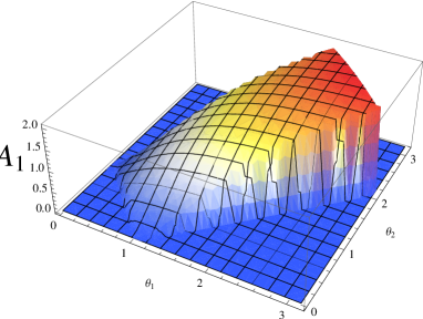
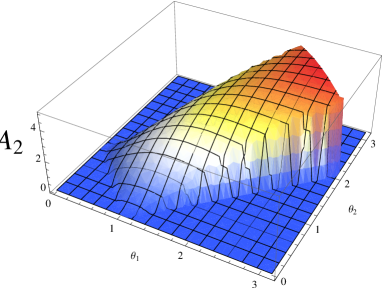
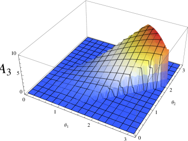
Figure 6: Shapes of $\mathcal{A}_{1}$, $\mathcal{A}_{2}$ and $\mathcal{A}_{3}$ with momentum configuration $k_{1}=k_{2}=k_{12}=k_{23}$ as function of $\theta_{1}$ and $\theta_{2}$. In this group of diagrams, parameters are chosen as $c_{\textrm{a}}=c_{\textrm{e}}=0.1$, $\epsilon=0.01$, $\lambda=\Pi=100$ and $T_{\mathcal{R}\mathcal{S}}=1$.

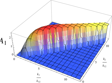
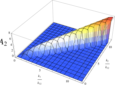
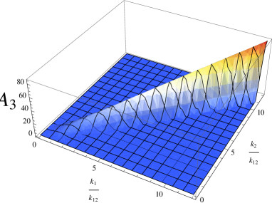
Figure 7: Shapes of $\mathcal{A}_{1}$, $\mathcal{A}_{2}$ and $\mathcal{A}_{3}$ with 2D momentum configuration $k_{1}=k_{2}=k_{12}$ as function of $k_{1}$ and $k_{2}$. In this group of diagrams, parameters are chosen as $c_{\textrm{a}}=c_{\textrm{e}}=0.1$, $\epsilon=0.01$, $\lambda=\Pi=100$ and $T_{\mathcal{R}\mathcal{S}}=1$.

6.3 Non-linear Parameters

In practice it is also convenient to define some so-called non-linear parameters, which characterize the typical or overall amplitudes of non-Gaussianities. For bispectrum which is defined as

$$\left\langle\mathcal{R}(\bm{k}_{1})\mathcal{R}(\bm{k}_{2})\mathcal{R}(\bm{k}_{3})\right\rangle=(2\pi)^{3}\delta^{3}(\bm{k}_{123})B(k_{1},k_{2},k_{3})\,,$$ (100)

the non-linear parameter $f_{\textrm{NL}}$ is usually defined as

$${}B(k_{1},k_{2},k_{3})\equiv\frac{6}{5}f_{\textrm{NL}}(k_{1},k_{2},k_{3})\left[P(k_{1})P(k_{2})+P(k_{2})P(k_{3})+P(k_{3})P(k_{1})\right]\,.$$ (101)

Note that in general $f_{\textrm{NL}}(k_{1},k_{2},k_{3})$ is a function of three momenta. (101) is motivated from the “local”-type bispectrum, which arises from interaction of the form as local product in real space:

$${}\mathcal{R}=\mathcal{R}_{\textrm{g}}+\frac{3}{5}f_{\textrm{NL}}^{\textrm{local}}\left(\mathcal{R}_{\textrm{g}}^{2}-\left\langle\mathcal{R}_{\textrm{g}}\right\rangle^{2}\right)\,,$$ (102)

where $\mathcal{R}_{\textrm{g}}$ is Gaussian. In this case, $f_{\textrm{NL}}$ is a pure real number, and the bispectrum is maximized in the limit of one of the three momenta going to zero. Although interaction of the form (102) is simple in real space, it is difficult to generate large local bispectrum in realistic models. Actually this form of non-Gaussianities are mostly produced by nonlinear gravitational evolution subsequent to the horizon-crossing [92, 93].

For trispectrum as defined in (92), the case is much more complicated. One possible parameterization is

$${}T(\bm{k}_{1},\bm{k}_{2},\bm{k}_{3},\bm{k}_{4})\equiv\tau_{\textrm{NL}}\left[P(k_{13})P(k_{3})P(k_{4})+\textrm{11 perms}\right]+\frac{54}{25}g_{\textrm{NL}}\left[P(k_{1})P(k_{2})P(k_{3})+\textrm{3 perms}\right]\,,$$ (103)

where $k_{ij}\equiv|\bm{k}_{i}+\bm{k}_{j}|$. This parameterization of trispectrum is also motivated by the “local-product-type” interaction in real space:

$${}\mathcal{R}\equiv\mathcal{R}_{\textrm{g}}+\frac{1}{2}\left(\tau_{\textrm{NL}}^{\textrm{local}}\right)^{\frac{1}{2}}\left(\mathcal{R}^{2}_{\textrm{g}}-\left\langle\mathcal{R}_{\textrm{g}}\right\rangle^{2}\right)+\frac{9}{25}g_{\textrm{NL}}^{\textrm{local}}\left(\mathcal{R}^{3}_{\textrm{g}}-3\mathcal{R}_{\textrm{g}}\left\langle\mathcal{R}^{2}_{\textrm{g}}\right\rangle\right)\,.$$ (104)

Actually, (103) itself has no prior convenience for the parameterization of trispectrum in general context. This is justified by the fact that, in models with non-canonical kinetic terms, especially with small speed(s) of sound, the leading-order non-Gaussianities are originated from the “derivative-coupled”-type interactions, which is obviously not real space “local-product”-type interactions described as (102) and (104).

Actually, there is a general definition of non-linear parameters for the trispectrum. From (93) and the discussion in sec.5.2.1, the trispectrum has dimension $\frac{H^{6}}{k^{9}}$, thus one may conveniently define a dimensionless non-linear parameter $\tau_{\textrm{NL}}$ by

$${}T_{\mathcal{R}}(\bm{k}_{1},\bm{k}_{2},\bm{k}_{3},\bm{k}_{4})\equiv(2\pi)^{6}\mathcal{P}_{\mathcal{R}}^{3}\frac{\tau_{\textrm{NL}}(\bm{k}_{1},\bm{k}_{2},\bm{k}_{3},\bm{k}_{4})}{F(\bm{k}_{1},\bm{k}_{2},\bm{k}_{3},\bm{k}_{4})}\,,$$ (105)

where $\mathcal{P}_{\mathcal{R}}$ is the power spectrum of curvature perturbation on large scales which is given in (50) and $F(\bm{k}_{1},\bm{k}_{2},\bm{k}_{3},\bm{k}_{4})$ is some function of momenta which has momentum dimension $k^{9}$. Remember that in general the so-called non-linear parameters $\tau_{\textrm{NL}}$ are always functions of momenta.

As addressed before, the non-linear parameter is essentially a characterization of the typical or overall amplitude of non-Gaussianities. Thus one may freely choose convenient $F(\bm{k}_{1},\bm{k}_{2},\bm{k}_{3},\bm{k}_{4})$ and momenta configurations to abstract real numbers for various purpose. In this work, in order to get a glance of the amplitude of non-Gaussianities from trispectrum, we abstract one real number $\tau^{\textrm{rth}}_{\textrm{NL}}$ from the trispectrum, which are defined respectively:

$${}\left.T_{\mathcal{R}}(\bm{k}_{1},\bm{k}_{2},\bm{k}_{3},\bm{k}_{4})\right|_{\textrm{regular tetrahedron}} \equiv(2\pi)^{6}\mathcal{P}_{\mathcal{R}}^{3}\frac{1}{k^{9}}\,\tau_{\textrm{NL}}^{\textrm{rth}}\,,$$ (106)

in which “regular tetrahedron” denotes the “regular tetrahedron” momenta configuration for trispectrum: $k_{1}=k_{2}=k_{3}=k_{4}=k_{12}=k_{23}\equiv k$ (see fig.5). Here we conveniently choose $F=k^{9}$. One can of course define other convenient non-linear parameters by choosing specific momentum configurations and $F$ in (105) for particular purpose.

As has been discussed in the end of sect.5.2.1, in multi-field case, the shape functions intrinsically involve parameters like $c_{\textrm{a}}$ etc. Thus, even the momentum configuration is fixed, the trispectrum or the corresponding non-linear parameters defined as in (106) is complicated. In this work we give the expression in the limit $c_{\textrm{a}}\ll 1$ and $c_{\textrm{e}}\ll 1$. We have

$$\tau_{\textrm{NL}}^{\textrm{rth}} =\left(1+T^{2}_{\mathcal{R}\mathcal{S}}\frac{c_{\textrm{a}}}{c_{\textrm{e}}}\right)^{-3}\left(\tau_{1}+\tau_{2}+\tau_{3}\right)\,,$$ (107)

where

$$\tau_{1} =-\frac{3c_{\textrm{a}}^{2}\left(54c_{\textrm{a}}^{2}\lambda^{2}-H^{2}\epsilon(3\lambda+10\Pi)\right)}{512H^{4}\epsilon^{2}}-T^{2}_{\mathcal{R}\mathcal{S}}\frac{9c_{\textrm{a}}\left(H^{2}\epsilon+3c_{\textrm{a}}^{4}\left(-7c_{\textrm{a}}^{2}+2c_{\textrm{e}}^{2}\right)\lambda\right)}{8(c_{\textrm{a}}+c_{\textrm{e}})^{5}H^{2}\epsilon}-T^{4}_{\mathcal{R}\mathcal{S}}\frac{9c_{\textrm{a}}\left(-13c_{\textrm{a}}^{2}+4c_{\textrm{e}}^{2}\right)}{1024c_{\textrm{e}}^{5}}\,,$$ (108)

$$\tau_{2} =\frac{13\left(-H^{2}\epsilon+3c_{\textrm{a}}^{4}\lambda\right)}{256c_{\textrm{a}}^{2}H^{2}\epsilon}+T^{2}_{\mathcal{R}\mathcal{S}}\frac{c_{\textrm{a}}^{3}\left(c_{\textrm{a}}^{2}+5c_{\textrm{a}}c_{\textrm{e}}+7c_{\textrm{e}}^{2}\right)\left(-H^{2}\epsilon+3c_{\textrm{a}}^{4}\lambda\right)}{4c_{\textrm{e}}^{4}(c_{\textrm{a}}+c_{\textrm{e}})^{5}H^{2}\epsilon}+T^{4}_{\mathcal{R}\mathcal{S}}\frac{13c_{\textrm{a}}(c_{\textrm{a}}^{2}-c_{\textrm{e}}^{4})}{256c_{\textrm{e}}^{7}}\,,$$

$$\tau_{3} =\frac{515}{8192c_{\textrm{a}}^{2}}+T^{2}_{\mathcal{R}\mathcal{S}}\frac{c_{\textrm{a}}\left(-5c_{\textrm{a}}^{2}+6c_{\textrm{e}}^{2}\right)\left(5c_{\textrm{a}}^{4}+25c_{\textrm{a}}^{3}c_{\textrm{e}}+43c_{\textrm{a}}^{2}c_{\textrm{e}}^{2}+25c_{\textrm{a}}c_{\textrm{e}}^{3}+5c_{\textrm{e}}^{4}\right)}{64c_{\textrm{e}}^{4}(c_{\textrm{a}}+c_{\textrm{e}})^{5}}-T^{4}_{\mathcal{R}\mathcal{S}}\frac{515c_{\textrm{a}}^{3}\left(c_{\textrm{a}}^{2}-c_{\textrm{e}}^{2}\right)}{2048c_{\textrm{e}}^{9}}\,.$$

7 Conclusion and Discussion

In this work, we studied the inflationary trispectrum in general multi-field models with scalar field Lagrangian of the form $P(X^{IJ},\phi^{I})$, which is the generalization of multi-field $k$-inflation and multi-field DBI models. In our general framework, we expanded the perturbation action up to the fourth-order, and calculated the four-point correlation functions for adiabatic and entropy modes, and also the trispectrum of the curvature perturbation on superhorizon scales.

We have shown that the perturbations for adiabatic and entropy modes are enhanced by $1/c_{\textrm{a}}$ and $1/c_{\textrm{e}}$ respectively, where $c_{\textrm{a}}$ and $c_{\textrm{e}}$ are propagation speeds of adiabatic and entropy modes respectively and in general $c_{\textrm{a}}\neq c_{\textrm{e}}$. In this work we focus on the trispectrum from four-point interaction vertices. In the two-field case, we have shown that there are three non-vanishing four-point correlation functions: $\left\langle Q_{\sigma}Q_{\sigma}Q_{\sigma}Q_{\sigma}\right\rangle$, $\left\langle Q_{\sigma}Q_{\sigma}Q_{s}Q_{s}\right\rangle$ and $\left\langle Q_{s}Q_{s}Q_{s}Q_{s}\right\rangle$. In the leading-order, all four-point correlation functions and also the final trispectrum of the curvature perturbation can be grouped into three types, which are deformations and permutations of three fundamental shape functions (69). These three types of contributions arise from three types of four-point interaction vertices. Thus, our result can be seen as the generalization of the previous results in general single-field models [22, 29, 31, 32] and also the very recent investigations in multi-DBI models [64].

In single-field models, one can always abstract momentum-dependent shape functions and put all other parameters as overall pre-factors. However, as we have seen in three “generalized shape functions” (88)-(90), parameters such as $c_{\textrm{a}}$, $c_{\textrm{e}}$, $\lambda$, $\Pi$ and $T_{\mathcal{R}\mathcal{S}}$ enter the definitions of these shape functions, and make the momentum dependence of these shape functions complicated. In this work, after a general discussion on the parameter-dependence of the trispectrum, we plot two set of shape diagrams of (88)-(90), including 3D and 2D momentum configuration with fixed parameters as $c_{\textrm{e}}$ etc. However, one expects that there should be better characterization of the trispectrum and the shape functions. We hope to get back to these issues in the future.

In this work we focus on the non-Gaussianities arising from the interactions among quantum fluctuations. While interactions not only cause non-Gaussianities, they also cause quantum loop-corrections. By collecting signatures of both quantum loop corrections and non-Gaussianities, we will obtain a more sensitive test of the physics of inflation [91].

In this work we focus on the primordial non-Gaussianities which are evaluated around the sound-horizon crossing. While detectable non-Gaussianities can also be produced when the curvature perturbation is generated from the entropy perturbation(s) on superhorizon scales, or at the end of inflation, or during the complicated reheating process. Since non-canonical kinetic terms can arise naturally in string theory inspired models, cosmic string effects should also be considered [114, 115].

Another issue should be address is that, in this work (and also previous works on non-Gaussianities in general multi-field models), the cross-correlation between adiabatic mode and entropy mode around horizon-crossing is assumed vanishing: $\left\langle Q_{\sigma}Q_{s}\right\rangle_{\ast}\approx 0$. This is good approximation in slow-roll inflation with canonical kinetic term, which corresponds to $\tilde{\xi}\approx 0$ in (46) and the background strategy is straight. In this work we also assume $\tilde{\xi}\approx 0$, while it is interesting to investigate the case where $\tilde{\xi}$ cannot be neglected and $\left\langle Q_{\sigma}Q_{s}\right\rangle_{\ast}\neq 0$ [103, 108, 109].

Acknowledgements

We would like to thank Qing-Guo Huang, Yi Wang for helpful discussions. XG thank Frederico Arroja and Kazuya Koyama for useful correspondence. This work was supported by the NSFC grant No.10535060/A050207, a NSFC group grant No.10821504 and Ministry of Science and Technology 973 program under grant No.2007CB815401.

Appendix A A Brief Review of “In-in” Formalism

A.1 Preliminaries

The “in-in formalism” (also dubbed as “Schwinger-Keldysh formalism”, or “Closed-time path formalism”) [110, 111, 112] is a perturbative approach for solving the evolution of expectation values over a finite time interval. It is therefore ideally suited not only to backgrounds which do not admit an S-matrix description, such as inflationary backgrounds.

In the calculation of S-matrix in particle physics, the goal is to determine the amplitude for a state in the far past $|\psi\rangle$ to become some state $|\psi^{\prime}\rangle$ in the far future,

$$\langle\psi^{\prime}|S|\psi\rangle=\langle\psi^{\prime}(+\infty)|\psi(-\infty)\rangle\,.$$

Here, conditions are imposed on the fields at both very early and very late times. This can be done because that in Minkowski spacetime, states are assumed to be non-interacting at far past and at far future, and thus are usually taken to be the free vacuum, i.e., the vacuum of the free Hamiltonian $H_{0}$. The free vacuum are assumed to be in “one-to-one” correspondence with the true vacuum of the whole interacting theory, as we adiabatically turn on and turn off the interactions between $t=-\infty$ and $t=+\infty$.

While the physical situation we are considering here is quite different. Instead of specifying the asymptotic conditions both in the far past and far future, we develop a given state forward in time from a specified initial time, which can be chosen as the beginning of inflation. In the cosmological context, the initial state is usually chosen as free vacuum, such as Bunch-Davis vacuum, since at very early times when perturbation modes are deep inside the Hubble horizon, according to the equivalence principle, the interaction-picture fields should have the same form as in Minkowski spacetime.

A.2 “In” vacuum

The Hamiltonian can be split into a free part and an interacting part: $H=H_{0}+H_{\textrm{i}}$. The time-evolution operator in the interacting picture is well-known

$${}U(\eta_{2},\eta_{1})=\mathrm{T}\exp\left(-i\int_{\eta_{1}}^{\eta_{2}}dt^{\prime}H_{\textrm{i}\textrm{I}}(\eta^{\prime})\right)\,,$$ (109)

where subscript “I” denotes interaction-picture quantities, T is the time-ordering operator. Our present goal is to relate the interacting vacuum at arbitrary time $|\Omega_{\textrm{I}}(t)\rangle$ to the free vacuum $|0_{\textrm{I}}\rangle$ (e.g., Bunch-Davis vacuum). The trick is standard. First we may expand $|\Omega_{\textrm{I}}(\eta)\rangle$ in terms of eigenstates of free Hamiltonian $H_{0}$, $|\Omega_{\textrm{I}}(\eta)\rangle=\sum_{n}|n_{\textrm{I}}\rangle\,\langle n_{\textrm{I}}|\Omega_{\textrm{I}}(\eta)\rangle$, then we evolve $|\Omega_{\textrm{I}}(\eta)\rangle$ by using (109)

$${}|\Omega_{\textrm{I}}(\eta_{2})\rangle=U(\eta_{2},\eta_{1})|\Omega_{\textrm{I}}(\eta_{1})\rangle=|0_{\textrm{I}}\rangle\,\langle 0_{\textrm{I}}|\Omega_{\textrm{I}}\rangle+\sum_{n\geq 1}e^{+iE_{n}(\eta_{2}-\eta_{1})}\,|n_{\textrm{I}}\rangle\,\langle n_{\textrm{I}}|\Omega_{\textrm{I}}(\eta_{1})\rangle\,.$$ (110)

From (110), we immediately see that, if we choose $\eta_{2}=-\infty(1-i\epsilon)$, all excited states in (110) are suppressed. Thus we relate interacting vacuum at $\eta=-\infty(1-i\epsilon)$ to the free vacuum $|0\rangle$ as

$$|\Omega_{\textrm{I}}(-\infty(1-i\epsilon))\rangle=|0_{\textrm{I}}\rangle\,\langle 0_{\textrm{I}}|\Omega_{\textrm{I}}\rangle$$ (111)

Thus, the interacting vacuum at arbitrary time $\eta$ is given by

$$|\textrm{VAC},\textrm{in}\rangle \equiv|\Omega_{\textrm{I}}(\eta)\rangle=U(\eta,-\infty(1-i\epsilon))|\Omega_{\textrm{I}}(-\infty(1-i\epsilon))\rangle$$ (112)

$$=\mathrm{T}\exp\left(-i\int^{\eta}_{-\infty(1-i\epsilon)}d\eta^{\prime}\,H_{\textrm{i}\textrm{I}}(\eta^{\prime})\right)|0_{\textrm{I}}\rangle\,\langle 0_{\textrm{I}}|\Omega_{\textrm{I}}\rangle\,.$$

A.3 Expectation values in “in-in” formalism

The expectation value of operator $\hat{\mathcal{O}}(\eta)$ at arbitrary time $\eta$ is evaluated as

$${}\langle\hat{\mathcal{O}}(\eta)\rangle \equiv\frac{\langle\textrm{VAC},\textrm{in}|\hat{\mathcal{O}}(\eta)|\textrm{VAC},\textrm{in}\rangle}{\langle\textrm{VAC},\textrm{in}|\textrm{VAC},\textrm{in}\rangle}$$ (113)

$$=\left\langle 0_{\textrm{I}}\left|\bar{\mathrm{T}}\exp\left(i\int^{\eta}_{-\infty{(1+i\epsilon)}}d\eta^{\prime}H_{1\textrm{I}}(\eta^{\prime})\right)\,\hat{\mathcal{O}}_{\textrm{I}}(\eta)\,\mathrm{T}\exp\left(-i\int^{\eta}_{-\infty{(1-i\epsilon)}}d\eta^{\prime}H_{\textrm{i}\textrm{I}}(\eta^{\prime})\right)\right|0_{\textrm{I}}\right\rangle\,,$$

where $\bar{\textrm{T}}$ is the anti-time-ordering operator.

For simplicity, we denote

$$-\infty(1-i\epsilon)\equiv-\infty^{+}\,,\qquad\qquad-\infty(1+i\epsilon)\equiv-\infty^{-}\,,$$ (114)

since, e.g., $-\infty^{+}$ has a positive imaginary part. Now let us focus on the time-order in (113). In standard S-matrix calculations, operators between $\langle 0|$ and $|0\rangle$ are automatically time-ordered. While in (113), from right to left, time starts from infinite past, or $-\infty^{+}$ precisely, to some arbitrary time $\eta$ when the expectation value is evaluated, then back to $-\infty^{-}$ again. This time-contour, which is shown in Fig.8, forms a closed-time path, so “in-in” formalism is sometimes called “closed-time path” (CTP) formalism.

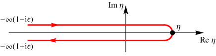
Figure 8: Closed-time path in “in-in” formalism.

A.4 Perturbation theory

The starting point of perturbation theory is the free theory two-point correlation functions. In canonical quantization procedure, we write a scalar field as

$$\phi_{\bm{k}}(\eta)=u(k,\eta)a_{\bm{k}}+u^{\ast}(k,\eta)a^{{\dagger}}_{-\bm{k}}\,,$$ (115)

where $u(k,\eta)$ is the mode function for $\phi_{\bm{k}}(\eta)$ (in practice, $u_{k}(\eta)$ and $u^{\ast}_{k}(\eta)$ are two linear-independent solutions of equation of motion for $\phi_{\bm{k}}(\eta)$, which are Wroskian normalized and satisfy some initial or asymptotic conditions ).

The free two-point function takes the form

$${}\left\langle 0\left|\phi_{\bm{k}_{1}}(\eta_{1})\phi_{\bm{k}_{2}}(\eta_{2})\right|0\right\rangle\equiv(2\pi)^{3}\delta^{3}(\bm{k}_{1}+\bm{k}_{2})G_{k_{1}}(\eta_{1},\eta_{2})\,,$$ (116)

with

$${}G_{k_{1}}(\eta_{1},\eta_{2})\equiv u_{k_{1}}(\eta_{1})u^{\ast}_{k_{1}}(\eta_{2})\,.$$ (117)

In this work, we take (116) and (117) as the starting point.

Now Taylor expansion of (113) gives

• 0th-order

  $${}\left\langle\hat{\mathcal{O}}(\eta)\right\rangle^{(0)}=\langle 0_{\textrm{I}}|\hat{\mathcal{O}}_{\textrm{I}}(\eta)|0_{\textrm{I}}\rangle\,.$$ (118)

• 1st-order (one interaction vertex)

  $${}\left\langle\hat{\mathcal{O}}(\eta)\right\rangle^{(1)}=2\,\textrm{Re}\left[-i\,\int^{\eta}_{{-\infty^{+}}}d\eta^{\prime}\,\left\langle 0_{\textrm{I}}\left|\hat{\mathcal{O}}_{\textrm{I}}(\eta)\,H_{\textrm{i}\textrm{I}}(\eta^{\prime})\right|0_{\textrm{I}}\right\rangle\right]\,.$$ (119)

• 2nd-order (two interaction vertices)

  $$\left\langle\hat{\mathcal{O}}(\eta)\right\rangle^{(2)} =-2\,\textrm{Re}\left[\int^{\eta}_{{-\infty^{+}}}d\eta^{\prime}\,\int^{\eta^{\prime}}_{{-\infty^{+}}}d\eta^{\prime\prime}\,\left\langle 0_{\textrm{I}}\left|\hat{\mathcal{O}}_{\textrm{I}}(\eta)\,H_{\textrm{i}\textrm{I}}(\eta^{\prime})\,H_{\textrm{i}\textrm{I}}(\eta^{\prime\prime})\right|0_{\textrm{I}}\right\rangle\right]$$ (120)

  $$\qquad\qquad+\int^{\eta}_{{-\infty^{-}}}d\eta^{\prime}\int^{\eta}_{{-\infty^{+}}}d\eta^{\prime\prime}\,\left\langle 0_{\textrm{I}}\left|H_{\textrm{i}\textrm{I}}(\eta^{\prime})\,\hat{\mathcal{O}}_{\textrm{I}}(\eta)\,H_{\textrm{i}\textrm{I}}(\eta^{\prime\prime})\right|0_{\textrm{I}}\right\rangle\,.$$

Here in this work, since we are considering four-point correlation functions from four-point vertices, (119) is needed.

Appendix B Various Expansion Quantities and Useful Relations

The exact form

$$P_{4} =P_{,\langle IJ\rangle}X^{IJ}_{4}+\frac{1}{2}\left[P_{,\langle IJ\rangle\langle KL\rangle}\left(X^{IJ}_{2}X^{KL}_{2}+2\,X^{(IJ}_{1}X^{KL)}_{3}\right)+2\,P_{,\langle IJ\rangle K}Q^{K}X^{IJ}_{3}\right]$$ (121)

$$\qquad+\left[\frac{1}{6}P_{,\langle IJ\rangle\langle KL\rangle\langle MN\rangle}\left(X^{IJ}_{2}X^{KL}_{1}X^{MN}_{1}+X^{KL}_{2}X^{MN}_{1}X^{IJ}_{1}+X^{MN}_{2}X^{IJ}_{1}X^{KL}_{1}\right)\right.$$

$$\qquad\qquad\qquad\left.+P_{,\langle IJ\rangle\langle KL\rangle M}Q^{M}\,X^{(IJ}_{1}X^{KL)}_{2}+\frac{1}{2}P_{,\langle IJ\rangle KL}Q^{K}Q^{L}\,X^{IJ}_{2}\right]$$

$$\qquad+\frac{1}{24}\left\{P_{,\langle IJ\rangle\langle KL\rangle\langle MN\rangle\langle PQ\rangle}\,(X^{IJ}_{1}X^{KL}_{1}X^{MN}_{1}X^{PQ}_{1})+4\,P_{,\langle IJ\rangle\langle KL\rangle\langle MN\rangle P}Q^{P}(X^{IJ}_{1}X^{KL}_{1}X^{MN}_{1})\right.$$

$$\qquad\qquad\left.+6\,P_{,\langle IJ\rangle\langle KL\rangle MN}Q^{M}Q^{N}(X^{IJ}_{1}X^{KL}_{1})+4\,P_{,\langle IJ\rangle KLM}Q^{K}Q^{L}Q^{M}\,X^{IJ}_{1}+P_{,IJKL}Q^{I}Q^{J}Q^{K}Q^{L}\right\}\,,$$

$$P_{3} =P_{,\langle IJ\rangle}X^{IJ}_{3}+\left[P_{,\langle IJ\rangle\langle KL\rangle}\,X^{(IJ}_{1}X^{KL)}_{2}+P_{,\langle IJ\rangle K}Q^{K}X^{IJ}_{2}\right]$$ (122)

$$\qquad+\frac{1}{6}P_{,\langle IJ\rangle\langle KL\rangle\langle MN\rangle}X^{IJ}_{1}X^{KL}_{1}X^{MN}_{1}$$

$$\qquad+\frac{1}{2}P_{,\langle IJ\rangle\langle KL\rangle M}Q^{M}X^{IJ}_{1}X^{KL}_{1}+\frac{1}{2}P_{,\langle IJ\rangle KL}Q^{K}Q^{L}X^{IJ}_{1}+\frac{1}{6}P_{,IJK}Q^{I}Q^{J}Q^{K}\,,$$

and

$$P_{2} =P_{,\langle IJ\rangle}\left\{-\frac{1}{2a^{2}}\partial_{i}Q^{I}\partial_{i}Q^{J}+\frac{1}{2}\left[\left(\dot{Q}^{I}\dot{Q}^{J}-2\,\dot{\phi}_{0}^{(I}N^{i}_{1}\partial_{i}Q^{J)}\right)-4\,\alpha_{1}\,\dot{\phi}_{0}^{(I}\dot{Q}^{J)}+\left(3\alpha_{1}^{2}-2\alpha_{2}\right)\,\dot{\phi}_{0}^{I}\dot{\phi}_{0}^{J}\right]\right\}$$ (123)

$$\qquad\qquad+\frac{1}{2}\left[P_{,\langle IJ\rangle\langle KL\rangle}\left(\dot{\phi}_{0}^{(I}\dot{Q}^{J)}-\alpha_{1}\,\dot{\phi}_{0}^{I}\dot{\phi}_{0}^{J}\right)\left(\dot{\phi}_{0}^{(K}\dot{Q}^{L)}-\alpha_{1}\,\dot{\phi}_{0}^{K}\dot{\phi}_{0}^{L}\right)\right.$$

$$\qquad\qquad\left.+2\,P_{,\langle IJ\rangle K}Q^{K}\left(\dot{\phi}_{0}^{(I}\dot{Q}^{J)}-\alpha_{1}\,\dot{\phi}_{0}^{I}\dot{\phi}_{0}^{J}\right)+P_{,IJ}Q^{I}Q^{J}\right]\,.$$

$$X^{IJ}_{4} =\frac{1}{2}\left(\partial^{i}\beta_{1}\partial_{i}Q^{I}\,\partial^{i}\beta_{1}\partial_{i}Q^{J}-2\,\dot{Q}^{(I}N_{2}^{i}\partial_{i}Q^{J)}\right)+2\alpha_{1}\left(\dot{Q}^{(I}\partial^{i}\beta_{1}\partial_{i}Q^{J)}+\dot{\phi}_{0}^{(I}N_{2}^{i}\partial_{i}Q^{J)}\right)$$ (124)

$$\qquad\qquad+\frac{1}{2}\left(3\alpha_{1}^{2}-2\alpha_{2}\right)\left(\dot{Q}^{I}\dot{Q}^{J}-2\,\dot{\phi}_{0}^{(I}\partial^{i}\beta_{1}\partial_{i}Q^{J)}\right)+\left(-4\alpha_{1}^{3}+6\alpha_{1}\alpha_{2}\right)\dot{\phi}_{0}^{(I}\dot{Q}^{J)}$$

$$\qquad\qquad+\frac{1}{2}\left(5\alpha_{1}^{4}-12\alpha_{1}^{2}\alpha_{2}+3\alpha_{2}^{2}\right)\dot{\phi}_{0}^{I}\dot{\phi}_{0}^{J}\,,$$

$$X^{IJ}_{3} =-\left(\dot{Q}^{(I}\partial^{i}\beta_{1}\partial_{i}Q^{J)}+\dot{\phi}_{0}^{(I}N_{2}^{i}\partial_{i}Q^{J)}\right)-\alpha_{1}\left(\dot{Q}^{I}\dot{Q}^{J}-2\,\dot{\phi}_{0}^{(I}\partial^{i}\beta_{1}\partial_{i}Q^{J)}\right)$$

$$\qquad\qquad+\left(3\alpha_{1}^{2}-2\alpha_{2}\right)\dot{\phi}_{0}^{(I}\dot{Q}^{J)}+\left(-2\alpha_{1}^{3}+3\alpha_{1}\alpha_{2}\right)\dot{\phi}_{0}^{I}\dot{\phi}_{0}^{J}\,,$$

$$X^{IJ}_{2} =-\frac{1}{2a^{2}}\partial_{i}Q^{I}\partial_{i}Q^{J}+\frac{1}{2}\left[\left(\dot{Q}^{I}\dot{Q}^{J}-2\,\dot{\phi}_{0}^{(I}N^{i}_{1}\partial_{i}Q^{J)}\right)-4\,\alpha_{1}\,\dot{\phi}_{0}^{(I}\dot{Q}^{J)}+\left(3\alpha_{1}^{2}-2\alpha_{2}\right)\,\dot{\phi}_{0}^{I}\dot{\phi}_{0}^{J}\right]\,.$$

In this work, at leading-order

$$X^{IJ}_{1} \simeq\dot{\phi}_{0}^{(I}\dot{Q}^{J)}\,,$$ (125)

$$X^{IJ}_{2} \simeq-\frac{1}{2a^{2}}\partial_{i}Q^{I}\partial_{i}Q^{J}+\frac{1}{2}\dot{Q}^{I}\dot{Q}^{J}\,.$$

Appendix C Interaction Hamiltonian

C.1 Derivation of interaction Hamiltonian

In this appendix, we show the explicit steps to get the interaction Hamiltonian. We start from the following leading-order Lagrangian (2nd, 3rd and 4th-order respectively):

$$\mathcal{L}_{2} =\frac{1}{2}\mathcal{K}_{mn}\dot{Q}_{m}\dot{Q}_{n}-\frac{1}{2a^{2}}\delta_{mn}\partial_{i}Q_{m}\partial_{i}Q_{n}\,,$$ (126)

$$\mathcal{L}_{3} =\frac{1}{2}\Xi_{mnl}\dot{Q}_{m}\dot{Q}_{n}\dot{Q}_{l}-\frac{1}{2a^{2}}\Upsilon_{mnl}\,\dot{Q}_{m}\partial_{i}Q_{n}\partial_{i}Q_{l}\,,$$

$$\mathcal{L}_{4} =\Gamma_{mnpq}\,\dot{Q}_{m}\dot{Q}_{n}\dot{Q}_{p}\dot{Q}_{q}-\frac{1}{4a^{2}}\Theta_{mnpq}\,\dot{Q}_{m}\dot{Q}_{n}\partial_{i}Q_{p}\partial_{i}Q_{q}+\frac{1}{8a^{4}}\Omega_{mnpq}\,\partial_{i}Q_{m}\partial_{i}Q_{n}\partial_{j}Q_{p}\partial_{j}Q_{q}\,.$$

The conjugate momentum of $Q_{m}$ is simply

$${}\pi_{m} \equiv\frac{\partial\mathcal{L}}{\partial\dot{Q}_{m}}$$ (127)

$$=\mathcal{K}_{mn}\dot{Q}_{n}+\frac{3}{2}\Xi_{mnl}\dot{Q}_{n}\dot{Q}_{l}-\frac{1}{2a^{2}}\Upsilon_{mnl}\partial_{i}Q_{n}\partial_{i}Q_{l}+4\Gamma_{mnpq}\dot{Q}_{n}\dot{Q}_{p}\dot{Q}_{q}-\frac{1}{2a^{2}}\Theta_{mnpq}\dot{Q}_{n}\partial_{i}Q_{p}\partial_{i}Q_{q}\,.$$

In order to get the Hamiltonian, we must solve $\dot{Q}_{m}$ in terms of its conjugate momentum $\pi_{m}$. In general, it is a complicated task. However, this can be done perturbatively. We make the ansatz:

$${}\dot{Q}_{m}\equiv\lambda^{(1)}_{mn}\,\pi_{n}+\lambda^{(2)}_{mnp}\,\pi_{n}\pi_{p}+\lambda^{(3)}_{mnpq}\,\pi_{n}\pi_{p}\pi_{q}+\mathcal{O}(\pi^{4})\,,$$ (128)

where $\lambda^{(i)}$’s are of order unity quantities, which we should determine in the following. Note that in (128), for our purpose, higher-order terms are not needed.

In order to determine $\lambda^{(i)}$’s in (128), the strategy is that, plug (128) into (127), and solve $\lambda^{(i)}$’s order-by-order.

$${}\pi_{m} \equiv\mathcal{K}_{mn}\left(\lambda^{(1)}_{np}\,\pi_{p}+\lambda^{(2)}_{npq}\,\pi_{p}\pi_{q}+\lambda^{(3)}_{npql}\,\pi_{p}\pi_{q}\pi_{l}\right)+\frac{3}{2}\Xi_{mnl}\left(\lambda^{(1)}_{np}\lambda^{(1)}_{lr}\,\pi_{p}\pi_{r}+2\lambda^{(1)}_{np}\lambda^{(2)}_{lrs}\,\pi_{p}\pi_{r}\pi_{s}\right)$$ (129)

$$\qquad-\frac{1}{2a^{2}}\Upsilon_{mnl}\,\partial_{i}Q_{n}\partial_{i}Q_{l}+4\Gamma_{mnpq}\,\lambda^{(1)}_{nl}\lambda^{(1)}_{pr}\lambda^{(1)}_{qs}\,\pi_{l}\pi_{r}\pi_{s}-\frac{1}{2a^{2}}\Theta_{mnpq}\,\lambda^{(1)}_{nl}\,\pi_{l}\partial_{i}Q_{p}\partial_{i}Q_{q}\,.$$

At first-order, in order to satisfy (129), we have

$$\pi_{m}\equiv\mathcal{K}_{mn}\,\lambda^{(1)}_{np}\,\pi_{p}\,,$$ (130)

this gives

$$\lambda^{(1)}_{mn}=\mathcal{K}^{-1}_{mn}\,.$$ (131)

At the second-order, (129) gives

$$\lambda^{(2)}_{spq}\,\pi_{p}\pi_{q} \equiv-\frac{3}{2}\Xi_{mnl}\mathcal{K}^{-1}_{sm}\mathcal{K}^{-1}_{np}\mathcal{K}^{-1}_{lr}\,\pi_{p}\pi_{r}+\frac{1}{2a^{2}}\Upsilon_{mnl}\mathcal{K}^{-1}_{sm}\partial_{i}Q_{n}\partial_{i}Q_{l}\,.$$ (132)

Fortunately, we do not need to solve $\lambda^{(2)}_{npq}$ explicitly, the above relation is enough for our purpose. Similarly, at the third-order we have

$$\quad\;\lambda^{(3)}_{spql}\,\pi_{p}\pi_{q}\pi_{l}$$ (133)

$$\equiv-3\Xi_{mnl}\mathcal{K}^{-1}_{ms}\mathcal{K}^{-1}_{np}\lambda^{(2)}_{lrs}\,\pi_{p}\pi_{r}\pi_{s}-4\Gamma_{mnpq}\mathcal{K}^{-1}_{ms}\mathcal{K}^{-1}_{nl}\mathcal{K}^{-1}_{pr}\mathcal{K}^{-1}_{qs}\,\pi_{l}\pi_{r}\pi_{s}+\frac{1}{2a^{2}}\Theta_{mnpq}\mathcal{K}^{-1}_{ms}\mathcal{K}^{-1}_{nl}\,\pi_{l}\partial_{i}Q_{p}\partial_{i}Q_{q}\,.$$

The fourth-order part of the Hamiltonian density is

$${}\mathcal{H}_{4}\equiv\pi_{m}\,\lambda^{(3)}_{mnpq}\,\pi_{n}\pi_{p}\pi_{q}-\mathcal{L}_{(4)}\,,$$ (134)

where $\mathcal{L}_{(4)}$ is the fourth-order part of the Lagrangian in terms of $Q_{m}$ and $\pi_{m}$ (note that $\mathcal{L}_{2}$, $\mathcal{L}_{3}$ and $\mathcal{L}_{4}$ all contribute to $\mathcal{L}_{(4)}$):

$$\mathcal{L}_{(4)} \equiv\mathcal{K}_{mn}\,\lambda^{(1)}_{np}\,\lambda^{(3)}_{mrst}\,\pi_{p}\pi_{r}\pi_{s}\pi_{t}+\frac{1}{2}\mathcal{K}_{mn}\,\lambda^{(2)}_{npq}\lambda^{(2)}_{mrs}\,\pi_{p}\pi_{q}\pi_{r}\pi_{s}+\frac{3}{2}\Xi_{mnl}\,\lambda^{(2)}_{mpq}\,\lambda^{(1)}_{nr}\lambda^{(1)}_{ls}\,\pi_{p}\pi_{q}\pi_{r}\pi_{s}$$ (135)

$$\qquad-\frac{1}{2a^{2}}\Upsilon_{mnl}\,\lambda^{(2)}_{mpq}\,\pi_{p}\pi_{q}\partial_{i}Q_{n}\partial_{i}Q_{l}+\Gamma_{mnpq}\,\lambda^{(1)}_{mr}\lambda^{(1)}_{ns}\lambda^{(1)}_{pu}\lambda^{(1)}_{qv}\,\pi_{r}\pi_{s}\pi_{u}\pi_{v}$$

$$\qquad-\frac{1}{4a^{2}}\Theta_{mnpq}\,\lambda^{(1)}_{mr}\lambda^{(1)}_{ns}\,\pi_{r}\pi_{s}\partial_{i}Q_{p}\partial_{i}Q_{q}+\frac{1}{8a^{4}}\Omega_{mnpq}\,\partial_{i}Q_{m}\partial_{i}Q_{n}\partial_{j}Q_{p}\partial_{j}Q_{q}\,.$$

Thus,

$$\mathcal{H}_{4} =-\frac{1}{2}\mathcal{K}_{mn}\,\lambda^{(2)}_{npq}\lambda^{(2)}_{mrs}\,\pi_{p}\pi_{q}\pi_{r}\pi_{s}-\frac{3}{2}\Xi_{mnl}\,\lambda^{(2)}_{mpq}\,\mathcal{K}^{-1}_{nr}\mathcal{K}^{-1}_{ls}\,\pi_{p}\pi_{q}\pi_{r}\pi_{s}$$ (136)

$$\qquad+\frac{1}{2a^{2}}\Upsilon_{mnl}\,\lambda^{(2)}_{mpq}\,\pi_{p}\pi_{q}\partial_{i}Q_{n}\partial_{i}Q_{l}-\Gamma_{mnpq}\,\mathcal{K}^{-1}_{mr}\mathcal{K}^{-1}_{ns}\mathcal{K}^{-1}_{pu}\mathcal{K}^{-1}_{qv}\,\pi_{r}\pi_{s}\pi_{u}\pi_{v}$$

$$\qquad+\frac{1}{4a^{2}}\Theta_{mnpq}\,\mathcal{K}^{-1}_{mr}\mathcal{K}^{-1}_{ns}\,\pi_{r}\pi_{s}\partial_{i}Q_{p}\partial_{i}Q_{q}-\frac{1}{8a^{4}}\Omega_{mnpq}\,\partial_{i}Q_{m}\partial_{i}Q_{n}\partial_{j}Q_{p}\partial_{j}Q_{q}\,.$$

C.2 Interaction Hamiltonian in the interaction picture

Now we go to the “interaction picture”, where all fields and momenta are “free”. The free (quadratic) part Hamiltonian density reads

$$\mathcal{H}_{0}^{\textrm{I}} =\pi_{m}^{\textrm{I}}\lambda^{(1)}_{mn}\pi_{n}^{\textrm{I}}-\mathcal{L}_{(2)}=\frac{1}{2}\mathcal{K}^{-1}_{mn}\,\pi_{m}^{\textrm{I}}\pi_{n}^{\textrm{I}}+\frac{1}{2a^{2}}\delta_{mn}\partial_{i}Q_{m}^{\textrm{I}}\partial_{i}Q_{n}^{\textrm{I}}\,.$$ (137)

Here we explicitly write superscript “I”, which denotes interaction picture quantities. In free theory, $\dot{Q}_{m}^{\textrm{I}}$ is related with $\pi_{m}^{\textrm{I}}$ by (remember that $\mathcal{H}_{0}^{\textrm{I}}\equiv\mathcal{H}_{0}$)

$$\dot{Q}_{m}^{\textrm{I}}\equiv\frac{\partial\mathcal{H}_{0}}{\partial\pi_{m}^{\textrm{I}}}=\mathcal{K}^{-1}_{mn}\pi_{n}^{\textrm{I}}\,,\qquad\qquad\textrm{i.e.}\qquad\pi_{m}^{\textrm{I}}=\mathcal{K}_{mn}\dot{Q}_{n}^{\textrm{I}}\,.$$ (138)

Now our task is to plug $\pi_{m}^{\textrm{I}}$ back into the fourth-order Hamiltonian (134), to get its “interaction picture form” $\mathcal{H}_{4}^{\textrm{I}}$. After a straightforward but rather tedious calculation, we get

$${}\mathcal{H}_{4}^{\textrm{I}} =\dot{Q}_{m}^{\textrm{I}}\dot{Q}_{n}^{\textrm{I}}\dot{Q}_{p}^{\textrm{I}}\dot{Q}_{q}^{\textrm{I}}\left[\frac{9}{8}\mathcal{K}^{-1}_{rs}\Xi_{rmn}\,\Xi_{spq}-\Gamma_{mnpq}\right]+\frac{1}{a^{2}}\dot{Q}_{m}^{\textrm{I}}\dot{Q}_{n}^{\textrm{I}}\partial_{i}Q_{p}^{\textrm{I}}\partial_{i}Q_{q}^{\textrm{I}}\left(\frac{1}{4}\Theta_{mnpq}-\frac{3}{4}\mathcal{K}^{-1}_{rs}\Upsilon_{rpq}\,\Xi_{smn}\right)$$ (139)

$$\qquad+\frac{1}{a^{4}}\partial_{i}Q_{m}^{\textrm{I}}\partial_{i}Q_{n}^{\textrm{I}}\partial_{j}Q_{p}^{\textrm{I}}\partial_{j}Q_{q}^{\textrm{I}}\left(\frac{1}{8}\mathcal{K}^{-1}_{rs}\Upsilon_{rmn}\,\Upsilon_{spq}-\frac{1}{8}\Omega_{mnpq}\right)\,.$$

We should keep in mind that the above $\mathcal{H}_{4}^{\textrm{I}}$ is the fourth-order interaction Hamiltonian in the “interaction picture”. In this work, we work in operator formalism in the interaction picture, thus, we use (139) as our staring point.

Appendix D Coefficients in $\mathcal{H}_{4}$

The various coefficients in the 4th-order interaction Hamiltonian density (62), (63) and (64) are

$$\Gamma_{\sigma} \equiv\frac{-H^{2}\epsilon(3\lambda+10\Pi)+54\lambda^{2}c_{a}^{2}}{24H^{6}\epsilon^{3}}\,,$$ (140)

$$\Gamma_{s} \equiv\frac{c_{a}^{4}\left(7-4c_{e}^{2}\right){}^{2}+4\left(c_{e}^{2}+c_{e}^{4}\right)+c_{a}^{2}\left(-13-20c_{e}^{2}+16c_{e}^{4}\right)}{16H^{2}\epsilon c_{a}^{2}c_{e}^{4}}\,,$$

$$\Gamma_{c} \equiv\frac{1}{4H^{4}\epsilon^{2}c_{a}^{4}c_{e}^{2}}\left[H^{2}\epsilon\left(-1+c_{e}^{2}\right){}^{2}+3\lambda c_{a}^{6}\left(-7+4c_{e}^{2}\right)+H^{2}\epsilon c_{a}^{2}\left(5-8c_{e}^{2}+4c_{e}^{4}\right)\right.$$

$$\qquad\qquad\qquad\qquad\left.+c_{a}^{4}\left(3H^{2}\epsilon+\left(-8H^{2}\epsilon+6\lambda\right)c_{e}^{2}+4H^{2}\epsilon c_{e}^{4}\right)\right]\,,$$

$$\Theta_{\sigma} \equiv\frac{-H^{2}\epsilon+H^{2}\epsilon c_{a}^{2}+3\lambda c_{a}^{4}}{4H^{4}\epsilon^{2}c_{a}^{2}}\,,$$ (141)

$$\Theta_{\sigma s} \equiv\frac{H^{2}\epsilon c_{a}^{2}+H^{2}\epsilon\left(-2+c_{e}^{2}\right)-3\lambda c_{a}^{4}\left(-2+c_{e}^{2}\right)}{4H^{4}\epsilon^{2}c_{a}^{2}c_{e}^{2}}\,,$$

$$\Theta_{s\sigma} \equiv\frac{5c_{a}^{2}-2c_{e}^{2}+c_{a}^{4}\left(-7+4c_{e}^{2}\right)}{8H^{2}\epsilon c_{a}^{2}c_{e}^{2}}\,,$$

$$\Theta_{s} \equiv\frac{-2c_{e}^{4}+c_{a}^{2}\left(2+9c_{e}^{2}-6c_{e}^{4}\right)+c_{a}^{4}\left(-14+15c_{e}^{2}-4c_{e}^{4}\right)}{8H^{2}\epsilon c_{a}^{2}c_{e}^{4}}\,,$$

$$\Theta_{c} \equiv-\frac{\left(-1+c_{e}^{2}\right)\left(c_{e}^{2}+2c_{a}^{2}\left(-1+c_{e}^{2}\right)\right)}{2H^{2}\epsilon c_{a}^{2}c_{e}^{2}}\,,$$

$$\Omega_{\sigma} \equiv\frac{-1+c_{a}^{2}}{16H^{2}\epsilon}\,,\qquad\qquad\Omega_{s}\equiv\frac{c_{a}^{2}\left(-2+c_{e}^{2}\right)^{2}+c_{e}^{2}\left(-4+3c_{e}^{2}\right)}{16H^{2}\epsilon c_{e}^{4}}\,,$$ (142)

$$\Omega_{\sigma s} \equiv-\frac{c_{e}^{2}+c_{a}^{2}\left(-2+c_{e}^{2}\right)}{8H^{2}\epsilon c_{e}^{2}}\,,\qquad\qquad\Omega_{c}\equiv\frac{-1+c_{e}^{2}}{4H^{2}\epsilon}\,.$$

Appendix E Explicit Expressions for $\left\langle Q_{\sigma}Q_{\sigma}Q_{s}Q_{s}\right\rangle_{i}$

$$\quad\;\left\langle Q_{\sigma}Q_{\sigma}Q_{s}Q_{s}\right\rangle_{2}$$ (143)

$$\equiv(2\pi)^{3}\delta^{3}(\bm{k}_{1234})\left(-2\Re\right)\left[4\Theta_{\sigma s}\,i\int_{-\infty}^{\eta_{\ast}}d\eta\,\left(-\bm{k}_{3}\cdot\bm{k}_{4}\right)\frac{\textrm{d}}{\textrm{d}\eta}G_{k_{1}}(\eta_{\ast},\eta)\frac{\textrm{d}}{\textrm{d}\eta}G_{k_{2}}(\eta_{\ast},\eta)F_{k_{3}}(\eta_{\ast},\eta)F_{k_{4}}(\eta_{\ast},\eta)\right]$$

$$=(2\pi)^{3}\delta^{3}(\bm{k}_{1234})\Theta_{\sigma s}\left(-\bm{k}_{3}\cdot\bm{k}_{4}\right)\frac{H^{8}c_{a}^{2}\,k_{1}^{2}k_{2}^{2}}{c_{e}^{2}\,\tilde{K}^{3}\prod_{i}^{4}k_{i}^{3}}\left[1+\frac{12\,c_{e}^{2}k_{3}k_{4}}{\tilde{K}^{2}}+\frac{3\,c_{e}\left(k_{3}+k_{4}\right)}{\tilde{K}}\right]$$

$$\quad\;\left\langle Q_{\sigma}Q_{\sigma}Q_{s}Q_{s}\right\rangle_{3}$$ (144)

$$\equiv(2\pi)^{3}\delta^{3}(\bm{k}_{1234})\left(-2\Re\right)\left[4\Theta_{s\sigma}\,i\int_{-\infty}^{\eta_{\ast}}d\eta\,\left(-\bm{k}_{1}\cdot\bm{k}_{2}\right)G_{k_{1}}(\eta_{\ast},\eta)G_{k_{2}}(\eta_{\ast},\eta)\frac{\textrm{d}}{\textrm{d}\eta}F_{k_{3}}(\eta_{\ast},\eta)\frac{\textrm{d}}{\textrm{d}\eta}F_{k_{4}}(\eta_{\ast},\eta)\right]$$

$$=(2\pi)^{3}\delta^{3}(\bm{k}_{1234})\Theta_{s\sigma}\left(-\bm{k}_{1}\cdot\bm{k}_{2}\right)\frac{H^{8}c_{e}^{2}\,k_{3}^{2}k_{4}^{2}}{c_{a}^{2}\,\tilde{K}^{3}\prod_{i}^{4}k_{i}^{3}}\left[1+\frac{12\,c_{a}^{2}k_{1}k_{2}}{\tilde{K}^{2}}+\frac{3\,c_{a}\left(k_{1}+k_{2}\right)}{\tilde{K}}\right]$$

$$\quad\;\left\langle Q_{\sigma}Q_{\sigma}Q_{s}Q_{s}\right\rangle_{4}$$ (145)

$$\equiv(2\pi)^{3}\delta^{3}(\bm{k}_{1234})\left(-2\Re\right)\left[\Theta_{c}\,i\int_{-\infty}^{\eta_{\ast}}d\eta\,\left(-\bm{k}_{2}\cdot\bm{k}_{4}\right)\frac{\textrm{d}}{\textrm{d}\eta}G_{k_{1}}(\eta_{\ast},\eta)G_{k_{2}}(\eta_{\ast},\eta)\frac{\textrm{d}}{\textrm{d}\eta}F_{k_{3}}(\eta_{\ast},\eta)F_{k_{4}}(\eta_{\ast},\eta)+\textrm{3 perms}\right]$$

$$=(2\pi)^{3}\delta^{3}(\bm{k}_{1234})\Theta_{c}\frac{H^{8}}{4\,\tilde{K}^{3}\prod_{i}^{4}k_{i}^{3}}\left[\left(-\bm{k}_{2}\cdot\bm{k}_{4}\right)k_{1}^{2}k_{3}^{2}\left(1+\frac{12c_{a}c_{e}k_{2}k_{4}}{\tilde{K}^{2}}+\frac{3\left(c_{a}k_{2}+c_{e}k_{4}\right)}{\tilde{K}}\right)+\textrm{3 perms}\right]$$

The other permutation is $(\bm{k}_{2},\bm{k}_{3})$, $(\bm{k}_{1},\bm{k}_{3})$ and $(\bm{k}_{1},\bm{k}_{4})$ combination.

$$\quad\;\left\langle Q_{\sigma}Q_{\sigma}Q_{s}Q_{s}\right\rangle_{5}$$ (146)

$$\equiv(2\pi)^{3}\delta^{3}(\bm{k}_{1234})\left(-2\Re\right)\left[4\Omega_{\sigma s}\left(\bm{k}_{1}\cdot\bm{k}_{2}\right)\left(\bm{k}_{3}\cdot\bm{k}_{4}\right)\,i\int_{-\infty}^{\eta_{\ast}}d\eta\,G_{k_{1}}(\eta_{\ast},\eta)G_{k_{2}}(\eta_{\ast},\eta)F_{k_{3}}(\eta_{\ast},\eta)F_{k_{4}}(\eta_{\ast},\eta)\right]$$

$$=(2\pi)^{3}\delta^{3}(\bm{k}_{1234})\Omega_{\sigma s}\frac{\left(\bm{k}_{1}\cdot\bm{k}_{2}\right)\left(\bm{k}_{3}\cdot\bm{k}_{4}\right)}{\tilde{K}}\left(-\frac{H^{8}}{c_{a}^{2}c_{e}^{2}\prod_{i}^{4}k_{i}^{3}}\right)$$

$$\qquad\times\left[1+\frac{12c_{a}^{2}c_{e}^{2}\prod_{i}^{4}k_{i}}{\tilde{K}^{4}}+\frac{3}{\tilde{K}^{3}}c_{a}c_{e}\left(c_{e}\left(k_{1}+k_{2}\right)k_{3}k_{4}+c_{a}k_{1}k_{2}\left(k_{3}+k_{4}\right)\right)\right.$$

$$\qquad\qquad\qquad\qquad\left.+\frac{1}{\tilde{K}^{2}}\left(c_{a}^{2}k_{1}k_{2}+c_{e}^{2}k_{3}k_{4}+c_{a}c_{e}\left(k_{1}+k_{2}\right)\left(k_{3}+k_{4}\right)\right)\right]$$

$$\quad\;\left\langle Q_{\sigma}Q_{\sigma}Q_{s}Q_{s}\right\rangle_{6}$$ (147)

$$\equiv(2\pi)^{3}\delta^{3}(\bm{k}_{1234})\left(-2\Re\right)\left[2\Omega_{c}\left(\bm{k}_{1}\cdot\bm{k}_{3}\right)\left(\bm{k}_{2}\cdot\bm{k}_{4}\right)\,i\int_{-\infty}^{\eta_{\ast}}d\eta\,G_{k_{1}}(\eta_{\ast},\eta)G_{k_{2}}(\eta_{\ast},\eta)F_{k_{3}}(\eta_{\ast},\eta)F_{k_{4}}(\eta_{\ast},\eta)+\textrm{1 perm}\right]$$

$$=(2\pi)^{3}\delta^{3}(\bm{k}_{1234})\Omega_{c}\,\frac{\left(\bm{k}_{1}\cdot\bm{k}_{3}\right)\left(\bm{k}_{2}\cdot\bm{k}_{4}\right)}{2\tilde{K}}\left(-\frac{H^{8}}{c_{a}^{2}c_{e}^{2}\prod_{i}^{4}k_{i}^{3}}\right)$$

$$\qquad\times\left[\left(1+\frac{12c_{a}^{2}c_{e}^{2}\prod_{i}^{4}k_{i}}{\tilde{K}^{4}}+\frac{3}{\tilde{K}^{3}}c_{a}c_{e}\left(c_{e}\left(k_{1}+k_{2}\right)k_{3}k_{4}+c_{a}k_{1}k_{2}\left(k_{3}+k_{4}\right)\right)\right.\right.$$

$$\qquad\qquad\left.\left.+\frac{1}{\tilde{K}^{2}}\left(c_{a}^{2}k_{1}k_{2}+c_{e}^{2}k_{3}k_{4}+c_{a}c_{e}\left(k_{1}+k_{2}\right)\left(k_{3}+k_{4}\right)\right)\right)+\textrm{1 perm}\right]\,.$$

References

- [1] E. Komatsu et al. [WMAP Collaboration], Astrophys. J. Suppl. 180, 330 (2009)
- [2] E. Komatsu et al., arXiv:0902.4759 [astro-ph.CO].
- [3] D. H. Lyth and A. Riotto, Phys. Rept. 314, 1 (1999) [arXiv:hep-ph/9807278].
- [4] N. Bartolo, E. Komatsu, S. Matarrese and A. Riotto, Phys. Rept. 402, 103 (2004) [arXiv:astro-ph/0406398].
- [5] V. F. Mukhanov, H. A. Feldman and R. H. Brandenberger, Phys. Rept. 215, 203 (1992).
- [6] R. H. Brandenberger, Lect. Notes Phys. 646, 127 (2004) [arXiv:hep-th/0306071].
- [7] J. M. Maldacena, JHEP 0305, 013 (2003) [arXiv:astro-ph/0210603].
- [8] V. Acquaviva, N. Bartolo, S. Matarrese and A. Riotto, Nucl. Phys. B 667, 119 (2003) [arXiv:astro-ph/0209156].
- [9] N. Bartolo, E. Komatsu, S. Matarrese and A. Riotto, Phys. Rept. 402, 103 (2004) [arXiv:astro-ph/0406398].
- [10] http://www.rssd.esa.int/index.php?project=Planck
- [11] L. Boubekeur and D. H. Lyth, Phys. Rev. D 73, 021301 (2006) [arXiv:astro-ph/0504046].
- [12] A. P. S. Yadav and B. D. Wandelt, Phys. Rev. Lett. 100, 181301 (2008) [arXiv:0712.1148 [astro-ph]].
- [13] K. M. Smith, L. Senatore and M. Zaldarriaga, arXiv:0901.2572 [astro-ph].
- [14] L. Senatore, K. M. Smith and M. Zaldarriaga, arXiv:0905.3746 [astro-ph.CO].
- [15] A. Curto, E. Martinez-Gonzalez and R. B. Barreiro, arXiv:0902.1523 [astro-ph.CO].
- [16] D. Nitta, E. Komatsu, N. Bartolo, S. Matarrese and A. Riotto, arXiv:0903.0894 [astro-ph.CO].
- [17] G. Rossmanith, C. Raeth, A. J. Banday and G. Morfill, arXiv:0905.2854 [astro-ph.CO].
- [18] E. Sefusatti, M. Liguori, A. P. S. Yadav, M. G. Jackson and E. Pajer, arXiv:0906.0232 [astro-ph.CO].
- [19] Y. Gong, X. Wang, Z. Zheng and X. Chen, arXiv:0904.4257 [astro-ph.CO].
- [20] D. Seery and J. E. Lidsey, JCAP 0506, 003 (2005) [arXiv:astro-ph/0503692].
- [21] X. Chen, M. x. Huang, S. Kachru and G. Shiu, JCAP 0701, 002 (2007) [arXiv:hep-th/0605045].
- [22] X. Chen, M. x. Huang and G. Shiu, Phys. Rev. D 74, 121301 (2006) [arXiv:hep-th/0610235].
- [23] C. Cheung, P. Creminelli, A. L. Fitzpatrick, J. Kaplan and L. Senatore, JHEP 0803, 014 (2008) [arXiv:0709.0293 [hep-th]].
- [24] X. Chen, R. Easther and E. A. Lim, JCAP 0706, 023 (2007) [arXiv:astro-ph/0611645].
- [25] X. Chen, R. Easther and E. A. Lim, JCAP 0804, 010 (2008) [arXiv:0801.3295 [astro-ph]].
- [26] D. Seery, J. E. Lidsey and M. S. Sloth, JCAP 0701, 027 (2007) [arXiv:astro-ph/0610210].
- [27] D. Seery and J. E. Lidsey, JCAP 0701, 008 (2007) [arXiv:astro-ph/0611034].
- [28] C. T. Byrnes, M. Sasaki and D. Wands, Phys. Rev. D 74, 123519 (2006) [arXiv:astro-ph/0611075].
- [29] F. Arroja and K. Koyama, Phys. Rev. D 77, 083517 (2008) [arXiv:0802.1167 [hep-th]].
- [30] D. Seery, M. S. Sloth and F. Vernizzi, JCAP 0903, 018 (2009) [arXiv:0811.3934 [astro-ph]].
- [31] X. Chen, B. Hu, M. x. Huang, G. Shiu and Y. Wang, arXiv:0905.3494 [astro-ph.CO].
- [32] F. Arroja, S. Mizuno, K. Koyama and T. Tanaka, arXiv:0905.3641 [hep-th].
- [33] F. Bernardeau and J. P. Uzan, Phys. Rev. D 67, 121301 (2003) [arXiv:astro-ph/0209330].
- [34] G. Dvali, A. Gruzinov and M. Zaldarriaga, Phys. Rev. D 69, 023505 (2004) [arXiv:astro-ph/0303591].
- [35] P. Creminelli, JCAP 0310, 003 (2003) [arXiv:astro-ph/0306122].
- [36] D. H. Lyth, JCAP 0511, 006 (2005) [arXiv:astro-ph/0510443].
- [37] L. Alabidi and D. Lyth, JCAP 0608, 006 (2006) [arXiv:astro-ph/0604569].
- [38] T. Suyama and F. Takahashi, JCAP 0809, 007 (2008) [arXiv:0804.0425 [astro-ph]].
- [39] H. R. S. Cogollo, Y. Rodriguez and C. A. Valenzuela-Toledo, JCAP 0808, 029 (2008) [arXiv:0806.1546 [astro-ph]].
- [40] Y. Rodriguez and C. A. Valenzuela-Toledo, arXiv:0811.4092 [astro-ph].
- [41] C. T. Byrnes, JCAP 0901, 011 (2009) [arXiv:0810.3913 [astro-ph]].
- [42] R. Holman and A. J. Tolley, JCAP 0805, 001 (2008) [arXiv:0710.1302 [hep-th]].
- [43] P. D. Meerburg, J. P. van der Schaar and P. S. Corasaniti, arXiv:0901.4044 [hep-th].
- [44] C. Armendariz-Picon, T. Damour and V. F. Mukhanov, Phys. Lett. B 458, 209 (1999) [arXiv:hep-th/9904075].
- [45] J. Garriga and V. F. Mukhanov, Phys. Lett. B 458, 219 (1999) [arXiv:hep-th/9904176].
- [46] E. Silverstein and D. Tong, Phys. Rev. D 70, 103505 (2004) [arXiv:hep-th/0310221].
- [47] X. Chen, Phys. Rev. D 71, 063506 (2005) [arXiv:hep-th/0408084].
- [48] X. Chen, JHEP 0508, 045 (2005) [arXiv:hep-th/0501184].
- [49] X. Chen, Phys. Rev. D 72, 123518 (2005) [arXiv:astro-ph/0507053].
- [50] S. Kecskemeti, J. Maiden, G. Shiu and B. Underwood, JHEP 0609, 076 (2006) [arXiv:hep-th/0605189].
- [51] J. E. Lidsey and D. Seery, Phys. Rev. D 75, 043505 (2007) [arXiv:astro-ph/0610398].
- [52] R. Bean, S. E. Shandera, S. H. Henry Tye and J. Xu, JCAP 0705, 004 (2007) [arXiv:hep-th/0702107].
- [53] H. V. Peiris, D. Baumann, B. Friedman and A. Cooray, Phys. Rev. D 76, 103517 (2007) [arXiv:0706.1240 [astro-ph]].
- [54] T. Kobayashi, S. Mukohyama and S. Kinoshita, JCAP 0801, 028 (2008) [arXiv:0708.4285 [hep-th]].
- [55] N. Bartolo, S. Matarrese and A. Riotto, Phys. Rev. D 65, 103505 (2002) [arXiv:hep-ph/0112261].
- [56] D. Seery and J. E. Lidsey, JCAP 0509, 011 (2005) [arXiv:astro-ph/0506056].
- [57] D. Langlois, S. Renaux-Petel, D. A. Steer and T. Tanaka, Phys. Rev. D 78, 063523 (2008) [arXiv:0806.0336 [hep-th]].
- [58] D. Langlois, S. Renaux-Petel, D. A. Steer and T. Tanaka, Phys. Rev. Lett. 101, 061301 (2008) [arXiv:0804.3139 [hep-th]].
- [59] D. Langlois, S. Renaux-Petel and D. A. Steer, JCAP 0904, 021 (2009) [arXiv:0902.2941 [hep-th]].
- [60] X. Gao, JCAP 0806, 029 (2008) [arXiv:0804.1055 [astro-ph]].
- [61] X. Gao and B. Hu, arXiv:0903.1920 [astro-ph.CO].
- [62] F. Arroja, S. Mizuno and K. Koyama, JCAP 0808, 015 (2008) [arXiv:0806.0619 [astro-ph]].
- [63] E. Kawakami, M. Kawasaki, K. Nakayama and F. Takahashi, arXiv:0905.1552 [astro-ph.CO].
- [64] S. Mizuno, F. Arroja, K. Koyama and T. Tanaka, arXiv:0905.4557 [hep-th].
- [65] J. L. Lehners and S. Renaux-Petel, arXiv:0906.0530 [hep-th].
- [66] C. T. Byrnes and G. Tasinato, arXiv:0906.0767 [astro-ph.CO].
- [67] F. Bernardeau and J. P. Uzan, Phys. Rev. D 66, 103506 (2002) [arXiv:hep-ph/0207295].
- [68] D. Wands, N. Bartolo, S. Matarrese and A. Riotto, Phys. Rev. D 66, 043520 (2002) [arXiv:astro-ph/0205253].
- [69] C. T. Byrnes, K. Y. Choi and L. M. H. Hall, JCAP 0810, 008 (2008) [arXiv:0807.1101 [astro-ph]].
- [70] C. T. Byrnes, K. Y. Choi and L. M. H. Hall, JCAP 0902, 017 (2009) [arXiv:0812.0807 [astro-ph]].
- [71] D. Langlois, F. Vernizzi and D. Wands, JCAP 0812, 004 (2008) [arXiv:0809.4646 [astro-ph]].
- [72] M. Kawasaki, K. Nakayama, T. Sekiguchi, T. Suyama and F. Takahashi, JCAP 0811, 019 (2008) [arXiv:0808.0009 [astro-ph]].
- [73] D. Langlois and S. Renaux-Petel, JCAP 0804, 017 (2008) [arXiv:0801.1085 [hep-th]].
- [74] G. I. Rigopoulos, E. P. S. Shellard and B. J. W. van Tent, Phys. Rev. D 73, 083521 (2006) [arXiv:astro-ph/0504508].
- [75] L. Alabidi, JCAP 0610, 015 (2006) [arXiv:astro-ph/0604611].
- [76] M. Sasaki, Prog. Theor. Phys. 120, 159 (2008) [arXiv:0805.0974 [astro-ph]].
- [77] A. Naruko and M. Sasaki, Prog. Theor. Phys. 121, 193 (2009) [arXiv:0807.0180 [astro-ph]].
- [78] Q. G. Huang, arXiv:0903.1542 [hep-th].
- [79] Q. G. Huang, arXiv:0904.2649 [hep-th].
- [80] C. Gordon, D. Wands, B. A. Bassett and R. Maartens, Phys. Rev. D 63, 023506 (2001) [arXiv:astro-ph/0009131].
- [81] B. A. Bassett, S. Tsujikawa and D. Wands, Rev. Mod. Phys. 78, 537 (2006) [arXiv:astro-ph/0507632].
- [82] D. A. Easson, R. Gregory, D. F. Mota, G. Tasinato and I. Zavala, JCAP 0802, 010 (2008) [arXiv:0709.2666 [hep-th]].
- [83] M. x. Huang, G. Shiu and B. Underwood, Phys. Rev. D 77, 023511 (2008) [arXiv:0709.3299 [hep-th]].
- [84] Y. F. Cai and W. Xue, arXiv:0809.4134 [hep-th].
- [85] Y. F. Cai and H. Y. Xia, arXiv:0904.0062 [hep-th].
- [86] X. Ji and T. Wang, arXiv:0903.0379 [hep-th].
- [87] S. Pi and T. Wang, arXiv:0905.3470 [astro-ph.CO].
- [88] X. Gao, arXiv:0903.1412 [astro-ph.CO].
- [89] X. Gao, arXiv:0904.4187 [hep-th].
- [90] X. Gao, Y. Wang, R. Brandenberger and A. Riotto, arXiv:0905.3821 [hep-th].
- [91] X. Gao and F. Xu, arXiv:0905.0405 [hep-th].
- [92] D. Babich, P. Creminelli and M. Zaldarriaga, JCAP 0408, 009 (2004) [arXiv:astro-ph/0405356].
- [93] D. H. Lyth and Y. Rodriguez, Phys. Rev. Lett. 95, 121302 (2005) [arXiv:astro-ph/0504045].
- [94] M. Sasaki, J. Valiviita and D. Wands, Phys. Rev. D 74, 103003 (2006) [arXiv:astro-ph/0607627].
- [95] K. A. Malik and D. H. Lyth, JCAP 0609, 008 (2006) [arXiv:astro-ph/0604387].
- [96] Q. G. Huang and Y. Wang, JCAP 0809, 025 (2008) [arXiv:0808.1168 [hep-th]].
- [97] Q. G. Huang, JCAP 0809, 017 (2008) [arXiv:0807.1567 [hep-th]].
- [98] Q. G. Huang, Phys. Lett. B 669, 260 (2008) [arXiv:0801.0467 [hep-th]].
- [99] S. Li, Y. F. Cai and Y. S. Piao, Phys. Lett. B 671, 423 (2009) [arXiv:0806.2363 [hep-ph]].
- [100] K. Ichikawa, T. Suyama, T. Takahashi and M. Yamaguchi, Phys. Rev. D 78, 023513 (2008) [arXiv:0802.4138 [astro-ph]].
- [101] T. Kobayashi and S. Mukohyama, arXiv:0905.2835 [hep-th].
- [102] D. H. Lyth, K. A. Malik and M. Sasaki, JCAP 0505, 004 (2005) [arXiv:astro-ph/0411220].
- [103] D. Langlois and F. Vernizzi, Phys. Rev. Lett. 95, 091303 (2005) [arXiv:astro-ph/0503416].
- [104] D. Langlois and F. Vernizzi, Phys. Rev. D 72, 103501 (2005) [arXiv:astro-ph/0509078].
- [105] D. Langlois and F. Vernizzi, JCAP 0702, 017 (2007) [arXiv:astro-ph/0610064].
- [106] S. Renaux-Petel and G. Tasinato, JCAP 0901, 012 (2009) [arXiv:0810.2405 [hep-th]].
- [107] A. A. Starobinsky and J. Yokoyama, arXiv:gr-qc/9502002.
- [108] C. T. Byrnes and D. Wands, Phys. Rev. D 74, 043529 (2006) [arXiv:astro-ph/0605679].
- [109] Z. Lalak, D. Langlois, S. Pokorski and K. Turzynski, JCAP 0707, 014 (2007) [arXiv:0704.0212 [hep-th]].
- [110] J. S. Schwinger, J. Math. Phys. 2 (1961) 407.
- [111] E. Calzetta and B. L. Hu, Phys. Rev. D 35, 495 (1987).
- [112] R. D. Jordan, Phys. Rev. D 33, 444 (1986).
- [113] E. Dimastrogiovanni and N. Bartolo, JCAP 0811, 016 (2008) [arXiv:0807.2790 [astro-ph]].
- [114] S. Sarangi and S. H. H. Tye, Phys. Lett. B 536, 185 (2002) [arXiv:hep-th/0204074].
- [115] C. J. Feng, X. Gao, M. Li, W. Song and Y. Song, Nucl. Phys. B 800, 190 (2008) [arXiv:0707.0908 [hep-th]].