Gravitational Wave Detection Using Redshifted $21$-cm Observations

Abstract

A gravitational wave traversing the line of sight to a distant source produces a frequency shift which contributes to redshift space distortion. As a consequence, gravitational waves are imprinted as density fluctuations in redshift space. The gravitational wave contribution to the redshift space power spectrum has a different $\mu$ dependence as compared to the dominant contribution from peculiar velocities. This, in principle, allows the two signals to be separated. The prospect of a detection is most favourable at the highest observable redshift $z$. Observations of redshifted $21$-cm radiation from neutral hydrogen (HI) hold the possibility of probing very high redshifts. We consider the possibility of detecting primordial gravitational waves using the redshift space HI power spectrum. However, we find that the gravitational wave signal, though present, will not be detectable on super-horizon scales because of cosmic variance and on sub-horizon scales where the signal is highly suppressed.

I Introduction

Primordial gravitational waves are a robust prediction of inflation grish ; star . These stochastic tensor perturbations are generated by the same mechanism as the matter density fluctuations, the ratio of the tensor perturbations to scalar perturbations being quantified through the tensor-to-scalar ratio ${r}$. Detecting the stochastic gravitational wave background is of considerable interest in cosmology since it carries valuable information about the very early universe. The cosmological background of gravitational wave has its signature imprinted on the CMBR temperature rubakov and polarization basko anisotropy maps. Current CMBR observations (WMAP-$5$ Year data) impose an upper bound ($r<0.43$) which is further tightened ($r<0.22$) if combined CMBR, BAO and SN data is used komatsu . Detecting the gravitational wave background is one of the important aims of upcoming PLANCK planck mission and future polarization based experiments like CMBPOL cmbpol .

A gravitational wave traversing the line of sight to a distant source will contribute to its redshift in addition to that caused by Hubble expansion and its peculiar velocity. This will produce a redshift space distortion in a manner similar to that caused by peculiar velocities kaiser . The effect arises due to the fact that distances are inferred from the spectroscopically measured redshifts. As a consequence, a gravitational wave will manifest itself as a density fluctuation in redshift space. In this paper we propose this as a possible technique to detect the primordial gravitational wave background.

While one could consider the possibility of detecting this at low redshifts ($z\sim 1$) using galaxy and quasar redshift surveys, we shall show that the prospects are much more favourable if the redshift is pushed to a value as high as possible.

Observations of redshifted $21$-cm radiation from neutral hydrogen (HI) can be used to measure the power spectrum of density fluctuations at very high redshifts extending all the way to the Dark Ages ($30<z<200$) zaldaloeb . Redshift space distortions make an important contribution to this signal bhaali . We investigate the possibility of using this to detect primordial gravitational waves. We note that the imprint of gravitational waves on the 21-cm signal from the Dark Ages has also been considered in an ealier work lewis .

II Formulation

The radial component of peculiar velocity introduces a redshift $z_{v}=v/c$ in excess of the cosmological redshift which arises due to the expansion of the universe. This distorts our view of the matter distribution in the three dimensional redshift space, where the radial distance is inferred from the measured redshift. As a consequence the density contrast $\delta=\delta\rho/\rho$ measured in redshift space $\delta^{s}$ is different from the actual density contrast $\delta^{r}$, and hamilton

$$\delta^{s}=\delta^{r}-\frac{c}{aH(a)}\frac{\partial z_{v}}{\partial x}$$ (1)

where $H(a)$ is the Hubble parameter and $x$ the comoving distance to the source. We see that any coherent velocity pattern (in-fall or outflow) manifests itself as a density fluctuation in redshift space. This takes a particularly convenient form in Fourier space if we assume that the peculiar velocities are produced by the density fluctuations $\delta^{r}$. We then have

$$\Delta^{s}({\bf k})=(1+f\mu^{2})\Delta^{r}({\bf k})$$ (2)

where $\Delta^{s}$ and $\Delta^{r}$ are the Fourier transforms of $\delta^{s}$ and $\delta^{r}$ respectively, $f=d\ln D/d\ln a\approx\Omega_{m}^{0.6}$, $D$ being the growing mode of density perturbations and $\mu=\hat{n}\cdot{\bf k}/k$ is the cosine of the angle between the line of sight ${\bf{\hat{n}}}$ and the wave vector ${\bf k}$. It follows that the power spectrum of density fluctuations in redshift space $P^{s}(k)$, is related to its real space counterpart $P^{r}(k)$ as kaiser

$$P^{s}({\bf k})=(1+f\mu^{2})^{2}P^{r}({\bf k})$$ (3)

A gravitational wave $h_{ab}(\vec{x},\eta)$ which is a tensor metric perturbation

$$ds^{2}=a^{2}\,\left[c^{2}\,d\eta^{2}-(\delta_{ab}+h_{ab})dx^{a}\,dx^{b}\right]$$ (4)

makes an additional contribution mukhanov

$$z_{h}=\frac{1}{2}n^{a}n^{b}\,\int_{\eta_{e}}^{\eta_{0}}h^{{}^{\prime}}_{ab}(\vec{x},\eta)\,d\eta\,$$ (5)

to the redshift along the line of sight of the unit vector $\hat{n}$. Here prime denotes a partial derivative with respect to $\eta$, $\eta_{e}$ and $\eta_{0}$ respectively refer to the photon being emitted and the present epoch when the photon is observed, and $\vec{x}=\hat{n}(\eta_{0}-\eta)$ is the photon’s spatial trajectory. Considering $z_{h}$ the gravitational wave contribution to the redshift, we have an additional contribution

$$\delta^{s}_{h}=-\frac{c}{aH}\frac{\partial z_{h}}{\partial x}$$ (6)

to $\delta^{s}$ the density contrast in redshift space (eq. 1). Simplifying this using $x=c(\eta_{0}-\eta_{e})$ we have

$$\delta^{s}_{h}=\frac{1}{2aH}n^{a}n^{b}\,h^{{}^{\prime}}_{ab}$$ (7)

We consider the primordial gravitational waves which we expand in Fourier modes as

$$h_{ab}(\vec{x},\eta)=\int\tilde{h}_{ab}({\bf k},\eta)e^{i{\bf k}\cdot\vec{x}}\frac{d^{3}{\bf k}}{(2\pi)^{3}}$$ (8)

and decompose $\tilde{h}_{ab}({\bf k},\eta)$ in terms of the two polarization tensors $e^{+}_{ab}$ and $e^{\times}_{ab}$ as tarunbharad

$$\tilde{h}_{ab}({\bf k},\eta)=h(k,\eta)\left[e^{+}_{ab}a^{+}({\bf k})+e^{\times}_{ab}a^{\times}({\bf k})\right]\frac{\sqrt{(2\pi)^{3}P_{h}(k)}}{2}\,.$$ (9)

Here $h(k,\eta)$ quantifies the temporal evolution, and $h(k,\eta)=3j_{1}(kc\eta)/(kc\eta)$ in a matter dominated universe, $j_{1}$ being the spherical Bessel function of order unity. The polarization tensors are normalized to $e^{+}_{ab}e^{+\,ab}=e^{\times}_{ab}e^{\times\,ab}=2$ and $e^{+}_{ab}e^{\times\,ab}=0$, $P_{h}(k)$ is the primordial gravitational wave power spectrum komatsu and $a^{\times}({\bf k}),a^{+}({\bf k})$ are Gaussian random variables such that

$$\langle\tilde{h}^{*}_{ab}({\bf k},\eta)\tilde{h}^{ab}({\bf k}^{{}^{\prime}},\eta)\rangle=(2\pi)^{3}\delta^{3}({\bf k}-{\bf k}^{{}^{\prime}})h^{2}(k,\eta)P_{h}(k)$$ (10)

Let us first consider a single Fourier mode of gravitational wave with ${\bf k}$ along the $z$ direction, and represent the line of sight as

$$\hat{n}=\sin\theta(\cos\phi\,\hat{i}+\sin\phi\,\hat{j})+\cos\theta\,\hat{k}\,.$$ (11)

We can than express eq. (7) as

$$\Delta^{s}({\bf k},\eta)=\frac{h^{{}^{\prime}}}{4aH}\sin^{2}\theta\left[\cos 2\phi\,a^{+}({\bf k})+\sin 2\phi\,a^{\times}({\bf k})\right]\sqrt{(2\pi)^{3}P_{h}(k)}\,.$$ (12)

This can be equivalently interpreted with $\hat{n}$ fixed and the direction of ${\bf k}$ varying. We use this to calculate $P^{s}_{h}({\bf k})$ the gravitational wave contribution to the power spectrum of density fluctuations in redshift space

$$P^{s}_{h}({\bf k})=\sin^{4}\theta\,\left\{\left[\frac{h^{{}^{\prime}}}{4aH}\right]^{2}\,\,P_{h}(k)\right\}$$ (13)

Thus the total power spectrum of density fluctuations in redshift space is

$$P^{s}({\bf k})=(1+f\mu^{2})^{2}P^{r}(k)+{(1-\mu^{2})}^{2}P^{r}_{h}(k)$$ (14)

where $P^{r}_{h}(k)$ refers to the terms in $\{\,\,\}$ in eq. (13). Here $P^{r}(k)$ and $P^{r}_{h}(k)$ are respectively the matter and gravitational wave contributions to the power spectrum of density fluctuations in redshift space. Both $P^{r}(k)$ and $P^{r}_{h}(k)$ are to be evaluated at the epoch corresponding to the redshift under observation.

The contributions from $P^{r}(k)$ and $P^{r}_{h}(k)$ have different $\mu$ dependence. This, in principle, can be used to separately estimate the gravitational wave and the matter contributions from the observed redshift space power spectrum. While the matter contribution is maximum when ${\bf k}$ and $\hat{n}$ are parallel, the gravitational wave contribution peaks when the two are mutually perpendicular.

III Results

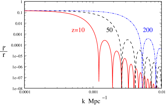
Figure 1: This shows the ratio $\tilde{r}/r$ at different $z$. This is predicted to have a constant value $\sim 0.16$ on super-horizon scales in the $\Omega_{m}=0.3$ LCDM model considered here.

We use $\tilde{r}=P^{r}_{h}(k)/P^{r}(k)$ to quantify the ratio of tensor perturbations to scalar perturbations in the redshift space power spectrum. Assuming $n_{s}=1$, $n_{T}\ll 1$, the value of $\tilde{r}$ is constant on super-horizon scales $(kc\eta\ll 1)$. This value is $\tilde{r}=r/4$ if $\Omega_{m}=1$, and somewhat smaller (Figure 1) with $\tilde{r}=0.16r$ for $\Omega_{m}=0.3$ in the LCDM model. Gravitational waves decay inside the horizon whereas matter perturbations grow on these scales. The ratio $\tilde{r}(k)$ is oscillatory and is severely suppressed on sub-horizon scales $(kc\eta\ll 1)$.

The prospect of detecting the gravitational wave signal is most favourable on super-horizon scales $(k\leq k_{\rm H}=(c\eta)^{-1})$. The $k$ range amenable for such observations (Figure 1) increases with redshift $z$ (smaller horizon $c\eta$). Observations of redshifted $21$-cm radiation hold the potential of measuring the redshift space power spectrum in the $z$ range $(30-200)$zaldaloeb ; bhaali , where the pre-reionization HI signal will be seen in absorption against the CMBR. Gravitational waves will make a $\sim r\times 16\%$ contribution to the HI signal on scales $k\leq k_{\rm H}$.

IV Feasibility of Detection

The cosmological HI signal will be buried in foregrounds bhaali1 ; santos ; mcquinn ; datta ; ali which are expected to be orders of magnitude larger than the signal. The foregrounds are continuum sources whose spectra are expected to be correlated over large frequency separations, whereas the HI signal, a line emission, is expected to be uncorrelated beyond a frequency separation. While this, in principle, can be used to separate the HI signal from the foregrounds, it should be noted that the frequency separation beyond which the HI signal becomes uncorrelated increases with $z$ and angular scale. This is a potential problem for the detection of the gravitational wave signal. In the subsequent discussion we have assumed that the foregrounds have been removed from the HI signal.

The distinctly different $\mu$ dependence of the scalar and gravitational wave components of the redshift space power spectrum can in principle be used to separate the two signals. Expressing the $\mu$ dependence barlo as $P^{s}(k,\mu)=P_{0}(k)+P_{2}(k)\mu^{2}+P_{4}(k)\mu^{4}$, the gravitational wave component can be estimated using $P_{h}^{r}(k)=[P_{0}(k)-P_{2}(k)]/2$. For a cosmic variance limited experiment, the error in $P_{2}(k)$ and $P_{0}(k)$ would be $\delta P(k)/P(k)\sim 1/\sqrt{N(k)}$ seo ; Mao ; mcquinn ; low ; pritch , where $N(k)$ denotes the number of ${\bf k}$ modes within the comoving volume of the survey. Thus $N(k)>\tilde{r}^{-2}\sim 10^{4}$ modes would be needed for a detection of the gravitational wave signal.

The number of modes with a comoving wave number between $k$ and $k+dk$ is $dN(k)=k^{2}\ dk\mathcal{V}/{(2\pi)}^{2}$, where $\mathcal{V}$ is the comoving survey volume. Assuming a survey between $z=20$ to $z=200$, and using a $k$ bin $dk=k/10$, we have $N(k)=10$ for $k=k_{\rm H}\sim 0.002\ {\rm Mpc}^{-1}$.

It is, in principle, possible to carry out HI observations in the entire $z$ range $z=0$ to $z=200$ bhaali1 and thereby increase the volume. Of the entire survey volume $\mathcal{V}_{0}$, for a mode $k$ only a volume $\mathcal{V}(k)=\mathcal{V}_{0}-(4\pi/3)(c\eta_{0}-k^{-1})^{3}$ where the mode is super-horizon contributes to the signal. Further, the largest mode $k_{max}$ is the one that entered the horizon at $z=200$, and the smallest mode $k_{min}$ has wavelength comparable to the radius of the survey volume. We then have, assuming a full sky survey,

$$N=(2\pi^{2})^{-1}\int_{k_{min}}^{k_{max}}\ \mathcal{V}(k)k^{2}dk$$ (15)

which gives $N\sim 100$. The number of independent modes is too small for a measurement at a level of precision that will allow the gravitational wave component to be detected. In conclusion, we note that the gravitational wave signal, though present, will not be detectable on super-horizon scales because of cosmic variance and on sub-horizon scales where the signal is highly suppressed.

References

- (1) Grishchuk, L.P.. Sov. Phys. JETP, 40, 409 (1975)
- (2) Starobinsky, A. A., Phys. Lett. B 91, 99 (1980)
- (3) Rubakov, V. A., Sazhin, M. V., & Veryaskin, A. V., Phys. Lett., B115, 189 (1982); Fabbri, R., & Pollock, M. d., Phys. Lett., B125, 445 (1983) ; Abott, L. F., & Wise, M. B., Nucl. Phys., B244, 541 (1984) ; Starobinsky, A. A., Sov. Astron. Lett., 11, 133 (1985); Souradeep, T., & Sahni, V., Modern Physics Letters A, 7, 3541 (1992); Crittenden, R., Bond, J. R., Davis, R. L., Efstathiou, G., & Steinhardt, P. J., Phys. Rev. Lett., 71, 324 (1993)
- (4) Basko, M. M., & Polnarev, A. G., MNRAS, 191, 207 (1980); Bond, J. R., & Efstathiou, G., ApJ, 285, L4 (1984); Crittenden, R., Bond, J. R., Davis, R. L., Efstathiou, G., & Steinhardt, P. J., Phys. Rev. Lett., 71, 324 (1993); Coulson, D., Crittenden, R. G., & Turok, N. G., Phys. Rev. Lett., 73, 2390 (1994)
- (5) Komatsu, E., et al., arXiv:0803.0547 (2008)
- (6) URL http://www.rssd.esa.int/index.php?project=planck
- (7) Baumann, D., et al., arXiv:0811.3919 (2008)
- (8) Kaiser, N., MNRAS, 227, 1 (1987)
- (9) Loeb, A., & Zaldarriaga, M., Physical Review Letters, 92, 211301 (2004)
- (10) Bharadwaj, S., & Ali, S. S., MNRAS, 352, 142 (2004)
- (11) Lewis, A., & Challinor, A. PRD, 76, 083005 (2007)
- (12) Hamilton, A. J. S. 1998, The Evolving Universe, 231, 185
- (13) Mukhanov, V., Physical foundations of cosmology, Cambridge University Press, pp 392 (2005)
- (14) Bharadwaj, S., Munshi, D., & Souradeep, T., PRD, 56, 4503 (1997)
- (15) Bharadwaj, S., & Ali, S. S., MNRAS, 356, 1519 ( 2005)
- (16) Santos, M. G., Cooray, A., & Knox, L. ApJ, 625, 575 (2005)
- (17) McQuinn, M., Zahn, O., Zaldarriaga, M., Hernquist, L., & Furlanetto, S. R. ApJ, 653, 815 ( 2006)
- (18) Datta, K. K., Choudhury, T. R., & Bharadwaj, S. MNRAS, 378, 119 (2007)
- (19) Ali, S. S., Bharadwaj, S., & Chengalur, J. N. MNRAS, 385, 2166 (2008)
- (20) Barkana, R., & Loeb, A. ApJL, 624, L65 (2005)
- (21) Seo, H.-J., & Eisenstein, D. J. , ApJ, 598, 720 (2003)
- (22) Mao, Y., Tegmark, M., McQuinn, M., Zaldarriaga, M., & Zahn, O. PRD, 78, 023529 (2008)
- (23) Loeb, A., & Wyithe, J. S. B. Physical Review Letters, 100, 161301 (2008)
- (24) Pritchard, J. R., & Loeb, A. , PRD, 78, 103511, (2008)