The Statistical Multifragmentation Model with Skyrme Effective Interactions

Abstract

The Statistical Multifragmentation Model is modified to incorporate the Helmholtz free energies calculated in the finite temperature Thomas-Fermi approximation using Skyrme effective interactions. In this formulation, the density of the fragments at the freeze-out configuration corresponds to the equilibrium value obtained in the Thomas-Fermi approximation at the given temperature. The behavior of the nuclear caloric curve at constant volume is investigated in the micro-canonical ensemble and a plateau is observed for excitation energies between 8 and 10 MeV per nucleon. A kink in the caloric curve is found at the onset of this gas transition, indicating the existence of a small excitation energy region with negative heat capacity. In contrast to previous statistical calculations, this situation takes place even in this case in which the system is constrained to fixed volume. The observed phase transition takes place at approximately constant entropy. The charge distribution and other observables also turn out to be sensitive to the treatment employed in the calculation of the free energies and the fragments’ volumes at finite temperature, specially at high excitation energies. The isotopic distribution is also affected by this treatment, which suggests that this prescription may help to obtain information on the nuclear equation of state.

I Introduction

Understanding the behavior of nuclear matter far from equilibrium, besides its intrinsic relevance to theoretical nuclear physics, is a subject of great interest to nuclear astrophysics, where the fate of supernovae or the properties of neutron stars are appreciably influenced by the nuclear equation of state (EOS) Bethe (1990); Dieperink et al. (2006); Lattimer and Prakash (2000). Thus, this area has been intensively investigated in different contexts during the last decades Dieperink et al. (2006); Lattimer and Prakash (2000); ter Haar and Malfliet (1987); Myers and Swiatecki (1998); Blaizot (1980); Shlomo and Youngblood (1994); Horowitz and schwenk (2006); Danielewicz et al. (2002); Li et al. (1997); Danielewicz et al. (1998). Nuclear collisions, at energies starting at a few tens of MeV per nucleon, provide a suitable means to study hot and compressed nuclear matter Danielewicz et al. (2002); Li et al. (1997); Danielewicz et al. (1998); Souza and Ngô (1993); Aichelin (1991); Viola et al. (2004); Bondorf et al. (1994); Bauer et al. (1993); Natowitz et al. (2002a). The determination of the nuclear caloric curve is of particular interest as it allows one to infer on the existence of a liquid-gas phase transition in nuclear matter. Nevertheless, owing to experimental difficulties, conflicting observations have been made in different experimental analyses Natowitz et al. (2002a); Ma et al. (2005); D’Agostino et al. (2002); Scharenberg et al. (2001); Campi et al. (1996); Ruangma et al. (2002); Das Gupta et al. (2001); Kwiatkowski et al. (1998); Serfling et al. (1998); Xi et al. (1998); Hauger et al. (1996); Ma et al. (1997); Moretto et al. (1996); Pochodzalla et al. (1995). Although there have been attempts to reconcile these results Natowitz et al. (2002b), this issue has not been settled.

The properties of the disassembling system in central collisions, as well as the outcome of the reactions, have been found to be fairly sensitive to the EOS employed in the many theoretical studies using dynamical models that have been performed Danielewicz et al. (2002); Aichelin (1991); Li et al. (1997); Danielewicz et al. (1998); Souza and Ngô (1993). However, in spite of their success in describing many features of the nuclear Multifragmentation process Bondorf et al. (1995); Das et al. (2005); Gross (1990), there has not been much effort to incorporate information based on the EOS in the main ingredients of statistical multifragmentation models. Yet, these models have recently been applied to investigate, for instance, the Isospin dependence of the nuclear energy at densities below the saturation value Le Fèvre et al. (2005); Iglio et al. (2006); Shetty et al. (2007). These calculations have suggested an appreciable reduction of the symmetry energy coefficient at low densities but other statistical calculations Raduta and Gulminelli (2007a, b); Souza et al. (2008) indicate that surface corrections to the symmetry energy may also explain the behavior observed in those studies. Therefore, statistical treatments, which consistently include density effects, are most advisable for these studies.

In this work, we modify the Statistical Multifragmentation Model (SMM) Bondorf et al. (1985a, b); Sneppen (1987) and calculate some of its key ingredients from the finite temperature Thomas-Fermi approximation Brack et al. (1985); Brack and Bhaduri (2003); Suraud and Vautherin (1984); Suraud (1987) using Skyrme effective interactions. This version of the model is henceforth labeled SMM-TF. The internal Helmholtz free energies of the fragments are calculated in a mean field approximation, which is fairly sensitive to the Skyrme force used Bonche et al. (1985). This makes possible to investigate whether such statistical treatments may provide information on the EOS. Furthermore, this approach allows to consistently take into account contributions to the free energy due to excitations in the continuum, in contrast to the traditional SMM Tan et al. (2003). For consistency with the mean field treatment, the equilibrium density of the fragments at the freeze-out stage is also provided by the Thomas-Fermi calculations. Thus, in contrast with former SMM calculations, fragments are allowed to be formed at densities below their saturation value. For a fixed freeze-out volume, this leads to a systematic reduction of the free volume, which directly affects the entropy of the fragmenting system, the fragment’s kinetic energies, and, also, the system’s pressure. As a consequence, other properties, such as the caloric curve and the multiplicities of the different fragment species produced, are also affected.

We have organized the remainder of this work as follows. In Sect. II we discuss the modifications to the SMM and present the results obtained with this modified treatment in Sect. III. Concluding remarks are drawn in Sect. IV. In Appendix A we provide a brief description of the Thomas-Fermi calculations employed in this work.

II Theoretical framework

In the SMM Bondorf et al. (1985a, b); Sneppen (1987), it is assumed that a source, made up of $Z_{0}$ protons and $A_{0}-Z_{0}$ neutrons, is formed at the late stages of the reaction, with total excitation energy $E^{*}$. This excited source then undergoes a simultaneous statistical breakup. As the system expands, there is a fast exchange of particles among the different fragments until a freeze-out configuration is reached, at which time particle exchange ceases and the composition of the primary fragments is well defined. One then assumes that thermal equilibrium has been reached and calculates the properties of the possible fragmentation modes through the laws of equilibrium statistical mechanics. A possible scenario consists in conjecturing that the freeze-out configuration is always attained when the system reaches a fixed pressure, i.e. the nuclear multifragmentation is an isobaric process. In this case, different statistical calculations predict a plateau in the caloric curve Bondorf et al. (1985b); Elliott and Hirsch (2000); Chomaz et al. (2000); Das et al. (2003); Gross (1997); Samaddar et al. (2004); Aguiar et al. (2006). The situation is qualitatively different if one assumes that, for a given source, the freeze-out configuration is reached at a fixed breakup volume $V_{\chi}$. As found in many different calculations, a monotonic increase of the temperature with excitation energy takes place in this case Souza et al. (2004); Bondorf et al. (1998); Aguiar et al. (2006). In what follows we demonstrate that this is a consequence of the properties assumed for the fragments formed, and not of the fixed volume assumption.

In this work we keep the breakup volume fixed for all fragmentation modes, and parametrize it through the expression:

$$V_{\chi}=(1+\chi)V_{0}\;,$$ (1)

where $V_{0}$ denotes the volume of the system at normal density and $\chi\geq 0$ is an input parameter.

In the micro-canonical version of SMM, the sampled fragmentation modes Sneppen (1987) are consistent with mass, charge, and energy conservation and thus the following constraints are imposed for each partition:

$$A_{0}=\sum_{A,Z}N_{A,Z}A\;,$$ (2)

$$Z_{0}=\sum_{A,Z}N_{A,Z}Z\;,$$ (3)

and

$$E_{\rm source}^{\rm g.s.}+E^{*}=E_{\rm trans}(T)+\sum_{A,Z}N_{A,Z}\left[-B_{A,Z}+\epsilon^{*}_{A,Z}\right]$$

$$+\frac{C_{\rm Coul}}{(1+\chi)^{1/3}}\frac{Z_{0}^{2}}{A_{0}^{1/3}}-\frac{C_{\rm Coul}}{(1+\chi)^{1/3}}\sum_{A,Z}N_{A,Z}\frac{Z^{2}}{A^{1/3}}\;.$$ (4)

In the above equations, $E_{\rm source}^{g.s.}$ is the ground state energy of the source, $N_{A,Z}$ denotes the multiplicity of fragments with mass and atomic numbers $A$ and $Z$, respectively, $B_{A,Z}$ corresponds to the binding energy of the fragment, and $\epsilon^{*}_{A,Z}(T)$ represents its excitation energy at temperature $T$. The Coulomb repulsion among the fragments is taken into account by the last two terms of the above equation which, together with the self energy contribution included in $B_{A,Z}$, give the Wigner-Seitz Wigner and Seitz (1934) approximation discussed in Ref. Bondorf et al. (1985a). The coefficient $C_{\rm Coul}$ is given in Ref. Souza et al. (2003). As discussed in Ref. Tan et al. (2003), the fragment’s binding energy $B_{A,Z}$ is either taken from experimental values Audi and Wapstra (1995) or is obtained from a careful extrapolation if empirical information is not available. The spin degeneracy factors, which enter in the calculation of the translational energy $E_{\rm trans}$, are also taken from experimental data for $A\leq 4$. In the case of heavier fragments, this factor is neglected, i.e., it is set to unity for all nuclei.

One should notice that the freeze-out temperature varies from one fragmentation mode $f=\{N_{A,Z}\}$ to another, since it is determined from the energy conservation constraint of Eq. (4). Therefore, the average temperature is calculated, as any other observable $O$, through the usual statistical averages:

$$\langle O\rangle=\frac{\sum_{f}O_{f}\exp(S_{f})}{\sum_{f}\exp(S_{f})}\;,$$ (5)

where $S_{f}$ denotes the entropy associated with the mode $f$. This entropy is calculated through the standard thermodynamical relation

$$S=-\frac{dF}{dT}\;,$$ (6)

where

$$F=E-TS$$ (7)

is the Helmholtz free energy. In the following, we write this quantity as

$$F=\sum_{A,Z}N_{A,Z}\left[-B_{A,Z}+f^{*}_{A,Z}(T)+f^{\rm trans}_{A,Z}(T)\right]+F_{\rm Coul}$$ (8)

where the contributions from the fragment’s internal excitation ($f^{*}_{A,Z}$) and translational motion ($f^{\rm trans}_{A,Z}$) are explicitly separated. The latter reads:

$$f_{A,Z}^{\rm trans}=-T\left[\log\left(\frac{g_{A,Z}V_{f}A^{3/2}}{\lambda_{T}^{3}}\right)-\frac{\log(N_{A,Z}!)}{N_{A,Z}}\right]\;.$$ (9)

In the above expression, $\lambda_{T}=\sqrt{\frac{2\pi\hbar^{2}}{m_{n}AT}}$ is the thermal wavelength, $m_{n}$ is the nucleon mass, $g_{A,Z}$ is the spin degeneracy factor, and $V_{f}$ denotes the free volume, i.e., it is the difference between $V_{\chi}$ and the volume occupied by all the fragments at freeze-out. The quantity $F_{\rm Coul}$ corresponds to the last two terms in Eq. (4).

Before we present the changes in the model associated with the Thomas-Fermi calculations, we briefly recall below the calculation of Helmholtz free energy $F$ in the SMM.

II.1 The standard SMM

In its original formulation Bondorf et al. (1985a), the SMM assumes that the diluted nuclear system undergoes a prompt breakup and that the resulting pieces of matter collapse to normal nuclear density, although being at temperature $T$. Therefore, the volume occupied by the fragments corresponds to $V_{0}$, so that

$$V_{f}=\chi V_{0}\;.$$ (10)

The energy and entropy associated with the translational motion of the fragment are respectively given by:

$$\epsilon^{\rm trans}_{A,Z}=f^{\rm trans}_{A,Z}+Ts^{\rm trans}_{A,Z}=\frac{3}{2}T$$ (11)

and

$$s^{\rm trans}_{A,Z} = -\frac{d}{dT}f^{\rm trans}_{A,Z}$$ (12)

$$= \frac{3}{2}+\log\left[\frac{g_{A,Z}V_{f}A^{3/2}}{\lambda_{T}^{3}}\right]-\frac{\log(N_{A,Z}!)}{N_{A,Z}}\;.$$

The internal free energy $f^{*}_{A,Z}$ has contributions from bulk and surface terms:

$$f^{*}_{A,Z}=-\frac{T^{2}}{\epsilon_{0}}A+\beta_{0}A^{2/3}\left[\left(\frac{T_{c}^{2}-T^{2}}{T_{c}^{2}+T^{2}}\right)^{5/4}-1\right]\;.$$ (13)

The values of the parameters in the above expression are $\epsilon_{0}=16.0$ MeV, $T_{c}=18.0$ MeV and $\beta_{0}=18.0$ MeV Tan et al. (2003). This expression is used for all nuclei with $A\geq 5$. Lighter fragments are assumed to behave as point particles, except for the alpha particle, for which one retains the bulk contribution to the free energy in order to take its excited states into account.

In Ref. Tan et al. (2003), the calculation of $f^{*}_{A,Z}$ has been modified to include empirical information on the excited states of light nuclei. We label this version of the model as ISMM and it is used throughout this work.

II.2 The SMM-TF

The Thomas-Fermi approximation, briefly outlined in Appendix A, allows one to calculate the internal free energy of the fragments $f^{*}_{A,Z}$ from Skyrme effective interactions. Equations (40,47) clearly show that $f^{*}_{A,Z}$ contains, besides those from the nuclear interaction traditionally used in SMM, contributions associated with the Coulomb energy in addition to the ones appearing in [Eq. (13)]. The additional Coulomb contribution arises, in the present case, because the equilibrium density of the nucleus at temperature $T$ does not correspond, in general, to its ground state value. This is illustrated in Fig. 1, which shows the ratio between the average density $\langle\rho\rangle$ at a temperature $T$, and the corresponding ground state value $\langle\rho_{0}\rangle$, for several selected light and intermediate mass nuclei. We define the sharp cutoff density $\langle\rho\rangle$ as that which gives the same root mean square radius as the actual nuclear density obtained in the Thomas-Fermi calculation. One observes that $\langle\rho\rangle$ decreases as one increases the temperature of the nucleus and that it quickly goes to zero as $T$ approaches its limiting temperature, since the nuclear matter tends to move to the external border of the box due to Coulomb instabilities Bonche et al. (1984, 1985); Suraud (1987). In our SMM-TF calculations presented below, we only accept a fragmentation mode at temperature $T$ if it is smaller than the limiting temperature of all the fragments of the partition. If this is not the case, the entire partition is discarded as not being physically possible and we sample another one.

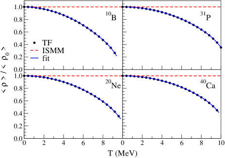
Figure 1: (Color online) Ratio between the average equilibrium density of the nucleus at temperature $T$ and the ground state value as a function of the temperature. For details, see the text.

Thus, a fragment’s volume at temperature $T$ is defined as:

$$\frac{V_{A,Z}}{V_{A,Z}^{0}}=\frac{\langle\rho_{0}^{A,Z}\rangle}{\langle\rho^{A,Z}\rangle}\;,$$ (14)

where $V_{A,Z}^{0}$ represents the ground state value. Since it is useful to have analytical formulae to use in practical SMM calculations, we performed a fit of $\langle\rho^{A,Z}\rangle$ using the following expression

$$\frac{\langle\rho^{A,Z}\rangle}{\langle\rho_{0}^{A,Z}\rangle}=1+T^{a_{n}^{A,Z}}\sum_{i=0}^{n-1}a_{i}^{A,Z}T^{i}\;,$$ (15)

where $\{a_{i}^{A,Z}\}$ are the fit parameters. This expression has proven to be accurate enough for numerical applications, as is illustrated in Fig. 1, which shows a comparison between Eq. (15) (full lines) and the results obtained with the Thomas-Fermi calculation (circles). The fit was carried out using $n=6$. The dashed lines emphasize the fact that $\langle\rho^{A,Z}\rangle=\langle\rho^{A,Z}_{0}\rangle$ in the standard SMM.

Instead of being given by Eq. (10), the free volume of a fragmentation mode now reads

$$V_{f}=(1+\chi)V_{0}-\sum_{A,Z}N_{A,Z}V^{0}_{A,Z}\left[1+T^{a_{n}^{A,Z}}\sum_{i=0}^{n-1}a_{i}^{A,Z}T^{i}\right]^{-1}\;.$$ (16)

For the values of $\chi$ usually adopted in statistical calculations ($0\leq\chi\leq 5$), this expression shows that, for some partitions, there may be a temperature $T_{V}$ for which $V_{f}\leq 0$. Therefore, if Eq. (4) leads to $T\geq T_{V}$, the partition is discarded as it is not a physically acceptable solution.

From Eq. (9), the entropy associated with the kinetic motion of the fragment $(A,Z)$ becomes

$$s^{\rm trans}_{A,Z}=\frac{3}{2}+\log\left[\frac{g_{A,Z}V_{f}A^{3/2}}{\lambda_{T}^{3}}\right]-\frac{\log(N_{A,Z}!)}{N_{A,Z}}+\frac{T}{V_{f}}\frac{dV_{f}}{dT}\;.$$ (17)

One should notice that, besides the smaller free volume, the last term in the above expression does not appear in the earlier version of the SMM. Since $dV_{f}/dT\leq 0$, the expression above gives a smaller contribution to the total entropy than Eq. (12). Owing to this change in the entropy, the average kinetic energy of the fragment becomes:

$$\epsilon_{A,Z}^{\rm trans}=\frac{3}{2}T\left(1+\frac{2}{3}\frac{T}{V_{f}}\frac{\partial V_{f}}{\partial T}\right)\;,$$ (18)

which, for a given temperature, is also lower than the corresponding SMM value. As a matter of fact, if the second factor dominates the first one, for $T>T_{K}$, where $\epsilon^{\rm trans}_{A,Z}(T_{K})=0$, it can even become negative. We also discard all partitions for which there is no solution of Eq. (4) satisfying $T<T_{K}$. This aspect is illustrated in Fig. 2, which shows the total kinetic energy $E_{\rm trans}$ as a function of $T$ for the ¹⁵⁰Nd nucleus, with $E^{*}/A=8$ MeV, for a partition containing $M=29$ fragments. The full line represents $E_{\rm trans}$, whereas the dashed line corresponds to the standard SMM formula. The factor, $M-1$ is due to the fact that the center of mass motion is consistently removed in all the kinetic formulae, although it is not explicitly stated above.

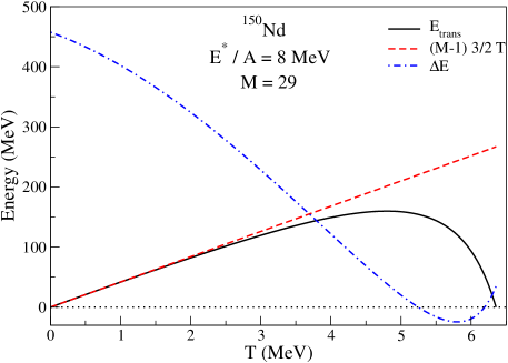
Figure 2: (Color online) Kinetic energy (full line) of a particular partition of the ¹⁵⁰Nd nucleus into $M=29$ fragments, for $E^{*}/A=8$ MeV and $V_{\chi}/V_{0}=3$, as a function of the temperature. For comparison, the standard average translational energy, $(M-1)\frac{3}{2}T$, is also displayed (dashed line). The difference between the left and the right hand sides of Eq. (4), $\Delta E$, is also shown (dashed-dotted line).

The observed drop of the kinetic energy may lead to nontrivial consequences. In the case of the ¹⁵⁰Nd nucleus and for $E^{*}/A\lesssim 7.0$ MeV, the fragment multiplicity is relatively low. Therefore, in this lower excitation energy range the behavior of the kinetic energy does not lead to any qualitative changes arising from the energy conservation constraint. However, for higher excitation energies, and consequently larger fragment multiplicities, the kinetic energy is comparable to the total energy of the system $E_{\rm total}$. In this case, for a given value of $E_{\rm total}$, there may be two values of $T$ which are acceptable solutions to Eq. (4). This is also illustrated in Fig. 2, which shows the difference $\Delta E$ between the left and the right hand sides of this expression. Since all the micro-states corresponding to the same total energy $E_{\rm total}$ should be included, both solutions, in this case associated with temperatures $T\approx 5.3$ MeV and $T\approx 6.2$ MeV must be considered. They contribute, however, with different statistical weights, due to the different number of states associated with each of these two solutions.

Based on this scenario, the determination of the freeze-out temperature from isotopic ratios Albergo et al. (1985), where one tacitly assumes that $T$ is univocally determined from $E^{*}$, should be carefully reexamined. To give a quantitative estimate of these effects, we show, in Fig. 3, the temperature distribution for the fragmentation of the ¹⁵⁰Nd nucleus, at $E^{*}/A=8$ MeV and $V_{\chi}=3V_{0}$. The full line in this picture shows the results when all the partitions are considered whereas the dashed line represents only those which lead to two different temperatures. The cases where there are two temperature solutions correspond to 43% of the events and account for 76% of the total statistical weight. These numbers are drastically changed at lower excitation energies where, for instance, one finds, at $E^{*}/A=6$ MeV, 0.03% and 0.09%, respectively. In spite of the great importance of these solutions at high excitation energy, the temperature distribution does not exhibit two clear dominant peaks, separated by a gap, as it could be expected from Fig. 2. This is because the numerical value of the two solutions vary from one partition to the other and the expected signature is thus blurred.

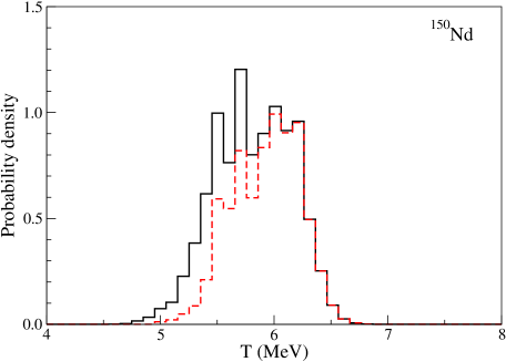
Figure 3: (Color online) Temperature distribution for the breakup of the the ¹⁵⁰Nd nucleus at $E^{*}/A=8$ MeV and for $V_{\chi}/V_{0}=3$. The full line corresponds to all events while those in which there are two temperatures associated with $E_{\rm total}$ are depicted by the dashed line.

We have also fitted the internal free energies of the nuclei through a simple analytical formula:

$$f_{A,Z}^{*}=-T^{2}\sum_{i=0}^{m}b_{i}^{A,Z}T^{i}\;,$$ (19)

where $\{b_{i}^{A,Z}\}$ are the fit coefficients. The results are depicted in Fig. 4 by the full lines, whereas the Thomas-Fermi calculations are represented by the circles. As in the previous case, an excellent agreement is obtained with a small number of parameters ($m=5$). The free energies used in the ISMM are also shown in this picture and are represented by the dashed lines. One sees that there are noticeable differences at low temperatures, in the case of the lighter nuclei. Particularly, many more states are suppressed in the ISMM than in the SMM-TF, which suggests that the latter should predict larger fragment multiplicities than the former. This is due to the empirical information on excited states which are taken into account in the ISMM Tan et al. (2003). In the case of heavier nuclei, the differences are more important at higher temperatures where the ISMM has more contributions from states in the continuum than the SMM-TF. However, the determination of the free energy at high temperatures in the ISMM is not as reliable as in the Thomas-Fermi approximation in the sense that the numerical values of the parameters $\epsilon_{0}$, $T_{c}$, and $\beta_{0}$, used in actual calculations, are not obtained from a fundamental theory. They correspond to average values Bondorf et al. (1985a, b) which, sometimes, are slightly changed by different authors Bondorf et al. (1985b); Tan et al. (2003); Botvina et al. (2002).

From the above parametrization to $f_{A,Z}^{*}$, the entropy and excitation energy associated with the fragment $(A,Z)$ read:

$$s^{*}_{A,Z}=2T\sum_{i=0}^{m}b_{i}^{A,Z}T^{i}+T^{2}\sum_{i=1}^{m}ib_{i}^{A,Z}T^{i-1}$$ (20)

and

$$\epsilon^{*}_{A,Z}=T^{2}\sum_{i=0}^{m}b_{i}^{A,Z}T^{i}+T^{3}\sum_{i=1}^{m}ib_{i}^{A,Z}T^{i-1}\;.$$ (21)

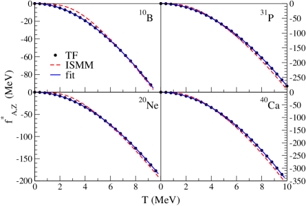
Figure 4: (Color online) Internal free energy of selected nuclei as a function of the temperature. For details, see the text.

The free energies and equilibrium volumes are calculated using the above expressions for alpha particles and all nuclei with $A\geq 5$.

III Results and discussion

The SMM-TF model described in the previous section is now applied to study the breakup of the ¹⁵⁰Nd nucleus at fixed freeze-out density. We use $V_{\chi}/V_{0}=3$ in all calculations below. The caloric curve of the system is displayed in Fig. 5. Besides the SMM-TF (circles) and the ISMM (triangles) results, the Thomas-Fermi calculations for the ¹⁵⁰Nd nucleus are also shown (dotted line), as well as the Fermi gas (full line) and the Maxwell-Boltzmann (dashed line) expressions. For $E^{*}/A\lesssim 8.0$ MeV, both SMM calculations agree fairly well on the prediction of the breakup temperatures. However, a kink in the caloric curve is observed at this point, in the case of the SMM-TF, indicating that the heat capacity of the system is negative within a small excitation energy range around this value. Negative heat capacities have been predicted by many calculations and have been strongly debated in the recent literature Bondorf et al. (1985b); Elliott and Hirsch (2000); Chomaz et al. (2000); Das et al. (2003); Gross (1997); Samaddar et al. (2004); Michaelian and Santamaría-Holek (2007); Lynden-Bell and Lynden-Bell (2008); Michaelian and Santamaría-Holek (2008a); Calvo et al. (2008); Michaelian and Santamaría-Holek (2008b). However, this feature is normally observed at the onset of the multifragment emission, i.e. at the beginning of the liquid-gas phase transition Bondorf et al. (1985b); Gross (1997), whereas it appears much later in the present calculation.

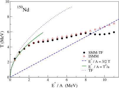
Figure 5: (Color online) Caloric curve associated with the breakup of the ¹⁵⁰Nd nucleus. The ISMM calculation of Ref. Tan et al. (2003) (triangles) and the SMM-TF calculation presented in this work (circles) are seen to differ for $E^{*}/A>8$ MeV. For reference the excitation energy of the compound nucleus calculated within the Fermi gas model (full line), the classical gas model (dashed line) as well as the Thomas-Fermi approach (dotted line) have also been presented. For further details, see the text.

In order to understand the qualitative differences between the two SMM approaches, we show, in Fig. 6, the multiplicity of light particles $N_{lp}$ (all particles with $A\leq 4$, except for alpha particles), the alpha particle $N_{\alpha}$ and the Intermediate Mass Fragment (IMF, $3\leq Z\leq 15$) $N_{IMF}$ multiplicities, as well as the total fragment multiplicity $N_{\rm total}$ as a function of the excitation energy. It is important to notice that neutrons are included in $N_{lp}$ and $N_{\rm total}$. One sees that there is a clear disagreement between the two SMM calculations in the prediction of the alpha particle multiplicity. This is due to the construction of the internal free energies in the ISMM Tan et al. (2003), which considers empirical low energy discrete states. Since the first excited state of the alpha particle is around 20 MeV, this strongly increases the free energy at low temperatures within the ISMM calculation, in contrast to the Thomas-Fermi model calculations. In the case of the other multiplicities, the agreement between the two model calculations is fairly good for excitation energies up to $E^{*}/A\approx 8$ MeV. The small discrepancy between $N_{\rm total}$ in the two calculations can be attributed to the differences in the alpha multiplicities. All multiplicities rise smoothly up to approximately this excitation energy. Then, at $E^{*}/A\approx 8$ MeV, in the SMM-TF calculations, $N_{\alpha}$ and $N_{IMF}$ reach a maximum and decrease from there on. This behavior is not observed in the case of the ISMM because it takes place beyond the energy range considered in the figure. Another feature also observed in this picture is the sudden change in the slope of the $N_{\rm total}$ and $N_{lp}$ multiplicities calculated using the SMM-TF model, which also takes place at the excitation energy mentioned above, and which is not seen in the ISMM results.

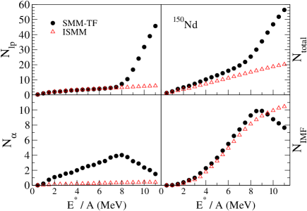
Figure 6: (Color online) Average multiplicity of light particles, alphas, IMF’s and the total fragment multiplicity, as a function of the excitation energy. For details, see the text.

Although the Helmholtz free energies of the fragments are somewhat different in both calculations, the differences are not large enough to quantitatively explain this peculiar behavior, as illustrated in Fig. 4. Therefore, the differences in the multiplicities calculated within the ISMM and SMM-TF models must be associated with the behavior of the kinetic terms, due to changes in the free volume in the SMM-TF calculations.

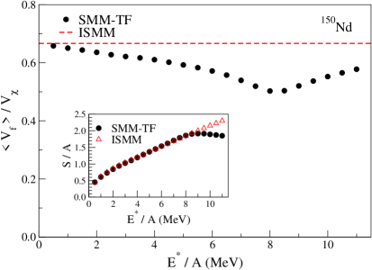
Figure 7: (Color online) Average free volume and entropy per nucleon as a function of the excitation energy calculated within the ISMM and SMM-TF models.

To examine this aspect more closely, we show, in Fig. 7, the energy dependence of $\langle V_{f}\rangle$. It confirms the expectation that $\langle V_{f}\rangle$ should decrease as $E^{*}$ increases, owing to the expansion of the fragments’ volumes at finite temperature. However, it reaches a minimum at $E^{*}/A\approx 8.0$ MeV and rises from this point on. The logarithmic volume term of the entropy [Eq. (17)] disfavors partitions with small free volumes. Furthermore, the last term in Eq. (17) also gets larger as $T$ increases since, besides being explicitly proportional to $T$, the factor $\mid\frac{dV_{f}}{dT}\mid$ grows faster at high temperatures, as it can be inferred from the behavior of the densities shown in Fig. 1. Therefore, the system favors the emission of very light particles, $N_{lp}$, which cannot become excited in our treatment, in order to minimize the reduction of $V_{f}$. Nevertheless, this preference is closely related to the energy conservation constraint given by Eq. (4). It is only when the excitation energy becomes sufficiently high that there is enough energy for the system to produce a significant number of very light particles. The inset in Fig. 7 shows the entropy per nucleon predicted by the two SMM treatments. It reveals that, while in the ISMM case it rises steadily, the entropy saturates, and even decreases in the SMM-TF model for $8.0\lesssim E^{*}/A\lesssim 11.0$ MeV. The large emission of particles which have no internal degrees of freedom prevents the entropy from falling off from this point on, since they lead to larger $\frac{dV_{f}}{dT}$ (smaller absolute values) by increasing $V_{f}$, as they do not expand. One should notice that the reduction of the complex fragment multiplicities does not mean that the limiting temperature of the fragments in the different partitions has been reached. In fact, the breakup temperatures obtained in the present calculations are much lower than the limiting temperatures of most nuclei, except for the very asymmetric ones, as may be seen in the examples given in Fig. 1 and in Refs. Bonche et al. (1985); Suraud (1987). This effect on the fragments produced should appear at much higher excitation energies, as those fragments have excitation energies much smaller than the original nucleus, since an appreciable amount of energy is used in the breakup of the system. Therefore, the back bending of the caloric curve and the small plateau observed in Fig. 5 are strongly ruled by the changes in the free volume. As a consequence of this fact, the phase transition at high excitation energy takes place at approximately constant entropy.

This observation is also corroborated by the charge distributions shown in Fig. 8 for four different excitation energies: $E^{*}/A=5$, 6, 7 and 8 MeV. It shows that the multiplicity of heavy fragments is strongly reduced in the SMM-TF calculations as the excitation energy increases, although they are not completely ruled out of the possible fragmentation modes. In particular, the SMM-TF model systematically gives much lighter fragments than the ISMM, for the reasons just discussed.

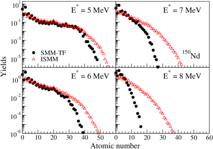
Figure 8: (Color online) Charge distribution in the breakup of the ¹⁵⁰Nd nucleus at four different excitation energies.

Even though the fragments are not directly affected by their limiting temperatures at the excitation energies we consider, the reduction of the entropy associated with the volume affects the fragment species in different ways. Indeed, since the proton rich nuclei tend to be more unstable, they are hindered due to these dilatation effects more strongly than the other isotopes. Owing to their larger volumes at a given temperature $T$, partitions containing proton rich fragments have smaller entropies than the others. Therefore, one should expect to observe a reduction in the yields of these fragments. This qualitative reasoning is confirmed by the results presented in Fig. 9, which displays the isotopic distribution of some selected light fragments, produced at $E^{*}/A=6.0$ MeV. One sees that, even though both SMM models make similar predictions for many observables at this excitation energy, the role played by the free volume effects just discussed is non-negligible. Since the limiting temperatures, as well as the equilibrium density at temperature $T$, is sensitive to the effective interaction used Bonche et al. (1985); Suraud (1987), these findings suggest that careful comparisons with experimental data may provide valuable information on the EOS.

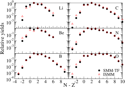
Figure 9: (Color online) Isotopic distribution of selected nuclear species produced in the breakup of the ¹⁵⁰Nd nucleus at $E^{*}/A=6.0$ MeV.

IV Concluding remarks

We have modified the SMM to incorporate the Helmholtz free energies and equilibrium densities of nuclei at finite temperature from the results obtained with the Thomas-Fermi approximation using Skyrme effective interactions. Owing to the reduction of the fragments’ translational energy at finite temperature, the model predicts the existence of two temperatures associated with the same total energy. This feature is directly associated with the reduction of the free volume due to the expansion of the fragments’ volumes. If this statistical treatment proves to be more appropriate to describe the nuclear multifragmentation process than its standard version, the determination of the isotopic temperatures, at high excitation energies, should be carefully reexamined, since one tacitly assumes a univocal relationship between the temperature and the excitation energy in the derivation that leads to the corresponding formulae Albergo et al. (1985).

The thermal dilatation of the fragments’ volumes also has important consequences on the fragmentation modes. For excitation energies larger than approximately 8 MeV per nucleon, it favors enhanced emission of particles which have no internal degrees of freedom (very light nuclei, protons and neutrons), leading to the onset of a gas transition at excitation energies around this value. The existence of a small kink in the caloric curve, as well as a plateau, for a system at constant volume is qualitatively different from the results obtained in previous SMM calculations where these features were observed only at (or at least at nearly) constant pressure Aguiar et al. (2006).

Since many-particle multiplicities, such as those associated with the IMF’s and the light particles, are very different in both statistical treatments for excitation energies larger than 8 MeV per nucleon, we believe that careful comparisons with experimental data may help to establish which treatment is better suited for describing the multifragment emission. Furthermore, since the isotopic distribution turns out to be sensitive to the treatment even at lower excitation energies, this suggests that one may obtain important information on the EOS by using different Skyrme effective interactions in the SMM-TF calculations. Particularly, this modified SMM model is appropriate to investigate the density dependence of the symmetry energy recently discussed Le Fèvre et al. (2005); Iglio et al. (2006); Shetty et al. (2007); Souza et al. (2008).

Appendix A The finite temperature Thomas-Fermi approximation

The Thomas-Fermi approximation to nuclear systems is thoroughly discussed in Refs. Brack et al. (1985); Brack and Bhaduri (2003); Suraud and Vautherin (1984); Suraud (1987). Thus, we review its essential features below in order to give a full account of all calculations presented in this work.

The equilibrium configuration of a nucleus at temperature $T$ is found by minimizing the thermodynamical potential $\Omega$ with respect to the number density $\rho_{\alpha}$ ($\alpha=p,n$ for protons or neutrons):

$$\Omega={\cal F}[\rho]-\sum_{\alpha}\int\;d^{3}\vec{r}\;\mu_{\alpha}\rho_{\alpha}$$ (22)

where the Helmholtz free energy is given by

$${\cal F}[\rho]=\int\left[{\cal H}_{\rm nucl}+{\cal H}_{\rm Coul}-T\sum_{\alpha}{\cal S}_{\alpha}\right]d^{3}\vec{r}\;.$$ (23)

In the above expression, ${\cal S}_{\alpha}$ denotes the entropy density associated with the species $\alpha$, $\mu_{\alpha}$ is the corresponding chemical potential, $\cal{H}_{\rm nucl}$ is the nuclear energy density of the system, and the Coulomb term reads:

$${\cal H}_{\rm Coul} = \frac{e^{2}}{2}\rho_{p}(\vec{r})\int\;\frac{\rho_{p}(\vec{r^{\prime}})}{\mid\vec{r}-\vec{r^{\prime}}\mid}\;d^{3}\vec{r^{\prime}}$$ (24)

$$- \frac{3}{4}e^{2}\left(\frac{3}{\pi}\right)^{1/3}\rho_{p}^{4/3}(\vec{r})\;.$$

The second term above corresponds to an approximation to the exchange contribution to the Coulomb energy Negele and Vautherin (1972); Titin-Schnaider and Quentin (1974).

The expression for $\cal{H}_{\rm nucl}$ given in Ref. Brack et al. (1985) may be rewritten as

$${\cal H}_{\rm nucl}={\cal H}_{0}+{\cal H}_{\tau}+{\cal H}_{\rm grad}+{\cal H}_{J}$$ (25)

where

$${\cal H}_{0} = \frac{t_{0}}{2}\left[(1+\frac{x_{0}}{2})\rho^{2}-(x_{0}+\frac{1}{2})(\rho_{n}^{2}+\rho_{p}^{2})\right]$$

$$+ \frac{t_{3}}{12}\rho^{\sigma}\left[(1+\frac{x_{3}}{2})\rho^{2}-(x_{3}+\frac{1}{2})(\rho_{n}^{2}+\rho_{p}^{2})\right]\,,$$

$${\cal H}_{\tau}=\frac{\hbar^{2}}{2m^{*}_{p}}\tau_{p}+\frac{\hbar^{2}}{2m^{*}_{n}}\tau_{n}\;,$$ (27)

$${\cal H}_{\rm grad} = \frac{1}{64}\left[9t_{1}-5t_{2}(1+\frac{4}{5}x_{2})\right]\left(\vec{\bigtriangledown}\rho\right)^{2}$$

$$- \frac{1}{64}\left[3t_{1}(1+2x_{1})+t_{2}(1+2x_{2})\right]\left(\vec{\bigtriangledown}\rho_{n}-\vec{\bigtriangledown}\rho_{p}\right)^{2}\;,$$

$${\cal H}_{J}=\frac{1}{2}W_{0}\left[\vec{J}\cdot\vec{\bigtriangledown}\rho+\vec{J}_{n}\cdot\vec{\bigtriangledown}\rho_{n}+\vec{J}_{p}\cdot\vec{\bigtriangledown}\rho_{p}\right]\;,$$ (29)

the total density is denoted by $\rho=\rho_{n}+\rho_{p}$ and $\vec{J}=\vec{J}_{p}+\vec{J}_{n}$ is the spin-orbit density. The kinetic factor $\tau_{\alpha}$ is given by

$$\tau_{\alpha}=\frac{1}{2\pi^{2}}\left(\frac{2m^{*}_{\alpha}}{\hbar^{2}}\right)^{5/2}T^{5/2}I_{3/2}(y_{\alpha})$$ (30)

where

$$\frac{\hbar^{2}}{2m^{*}_{\alpha}} = \frac{\partial}{\partial\tau_{\alpha}}{\cal H}_{\rm nucl}$$ (31)

$$= \frac{\hbar^{2}}{2m}+\frac{1}{8}\left[t_{1}(1-x_{1})+3t_{2}(1+x_{2})\right]\rho_{\alpha}$$

$$+ \frac{1}{4}\left[t_{1}(1+\frac{x_{1}}{2})+t_{2}(1+\frac{x_{2}}{2})\right]\rho_{\alpha^{\prime}}$$

and $\rho_{\alpha^{\prime}}=\rho_{p}\,(\rho_{n})$ if $\alpha=n\,(p)$. The Fermi-Dirac integral

$$I_{n/2}(y)=\int_{0}^{\infty}\;dx\;\frac{x^{n/2}}{1+\exp(x-y)}$$ (32)

is efficiently calculated using the formulae given in Ref. Antia (1993), where one also finds approximations to the inverse function $y(I_{n/2})$. The latter is determined from the number density

$$\rho_{\alpha}=\frac{1}{2\pi^{2}}\left(\frac{2m^{*}_{\alpha}}{\hbar^{2}}\right)^{3/2}T^{3/2}I_{1/2}(y_{\alpha})\;.$$ (33)

The entropy density ${\cal S}_{\alpha}$ can then be easily calculated

$${\cal S}_{\alpha}=\frac{5}{3}\frac{\hbar^{2}}{2m^{*}_{\alpha}}\frac{\tau_{\alpha}}{T}-\rho_{\alpha}y_{\alpha}\;.$$ (34)

The parameter set $\{x_{i},t_{i},\sigma,W_{0}\}$, $i=0,1,2,3$, for the Skyrme interaction used in this work, SKM, is listed in Ref. Brack et al. (1985). Since we stay in the zero-th order approximation in $\hbar$, $\vec{J}_{\alpha}=0$ and then ${\cal H}_{J}$ does not contribute to $\cal{H}_{\rm nucl}$ Brack et al. (1985).

Following Suraud and Vautherin Suraud and Vautherin (1984); Suraud (1987), the equilibrium configuration is found by iterating the densities at the k-th step according to

$$\rho^{(k+1)}_{\alpha}=\rho^{(k)}_{\alpha}\left[1-\lambda\left(B^{(k)}_{\alpha}-\mu^{(k)}_{\alpha}\right)\right]$$ (35)

where

$$\mu^{(k)}_{\alpha}=\frac{1}{N_{\alpha}}\int\;d^{3}\vec{r}\;B^{(k)}_{\alpha}(\vec{r})\rho^{(k)}_{\alpha}(\vec{r}),$$ (36)

$N_{p}=Z$, $N_{n}=A-Z$, and

$$B^{(k)}_{\alpha}=\frac{\delta{\cal F}}{\delta\rho^{(k)}_{\alpha}}\;.$$ (37)

The parameter $\lambda$ is chosen to be small enough in order to ensure that the first order approximation given by Eq. (35) remains valid.

In our numerical implementation, we have assumed spherical symmetry, and discretized the space using a mesh spacing $\Delta R=0.1$ fm, which suffices for our purposes. As suggested in Refs. Suraud and Vautherin (1984); Suraud (1987), the second term of Eq. (A) is neglected since it is small and may lead to numerical instabilities. Similarly to the treatment adopted in Ref. Suraud and Vautherin (1984), the gradient density terms are calculated at the mesh point $r_{i+1/2}=(i+1/2)\Delta R$, using Koonin and Meredith (1990)

$$\frac{\partial}{\partial r}\rho(r_{i+1/2})=\frac{\rho(r_{i})-\rho(r_{i-1})}{2(\Delta R/2)}+{\cal O}[(\Delta R)^{2}]\;,$$ (38)

which turned out to be numerically stable.

Due to the important contributions associated with unbound states at high temperatures, the above treatment is not accurate for $T\gtrsim 4$ MeV, as pointed out by Bonche, Levit, and Vautherin Bonche et al. (1984). Therefore, these authors have proposed a method to extend the Hartree-Fock calculations to higher temperatures. As they have noticed, there are two solutions of the Hartree-Fock equations for a given chemical potential. One of them corresponds to a nucleus in equilibrium with its evaporated particles whereas the other is associated with the nucleon gas. Thus, in their formalism, the properties of the hot nucleus is obtained by subtracting the thermodynamical potential associated with an introduced nucleon gas $\Omega_{G}$ from that corresponding to the nucleus in equilibrium with its evaporated gas $\Omega_{NG}$. Except for the Coulomb energy, there is no interaction between the gas and the nucleus-gas system.

This approach has been successfully applied by these authors Bonche et al. (1984, 1985) and has been adapted to the finite temperature Thomas-Fermi approximation by Suraud Suraud (1987). More precisely, the thermodynamical potential associated with the nucleus is given by

$$\Omega_{N}=\Omega_{NG}-\Omega_{G}+E_{\rm Coul}\;.$$ (39)

One should notice that, by construction, $\Omega_{NG}$ and $\Omega_{G}$ do not contain any Coulomb contribution. More specifically, one defines the subtracted free energy

$${\cal F}^{\rm sub} = \int\;\left[{\cal H}_{\rm nucl}^{NG}-{\cal H}_{\rm nucl}^{G}-T\sum_{\alpha}\left({\cal S}_{\alpha}^{NG}-{\cal S}_{\alpha}^{G}\right)\right]\;d^{3}\vec{r}$$ (40)

$$+ \int\;{\cal H}_{\rm Coul}^{\rm sub}\;d^{3}\vec{r}$$

where the subtracted Coulomb energy density, in the last term of this expression, reads

$${\cal H}_{\rm Coul}^{\rm sub} \equiv \frac{e^{2}}{2}\rho_{p}(\vec{r})\int\;d^{3}\vec{r^{\prime}}\frac{\rho_{p}(\vec{r^{\prime}})}{\mid\vec{r}-\vec{r^{\prime}}\mid}$$ (41)

$$- \frac{3}{4}e^{2}\left(\frac{3}{\pi}\right)^{1/3}\left[\left(\rho^{NG}_{p}\right)^{4/3}-\left(\rho^{G}_{p}\right)^{4/3}\right]\;,$$

and the subtracted density $\rho_{p}$:

$$\rho_{p}(\vec{r})=\rho_{p}^{NG}(\vec{r})-\rho_{p}^{G}(\vec{r})$$ (42)

is the quantity that enters in the direct part of the Coulomb energy.

The iteration scheme given by Eq. (35) remains unchanged if one rewrites $B_{\alpha}^{(k)}$ as

$$B_{\alpha}^{(k,\gamma)}=\pm\frac{\delta{\cal F}^{\rm sub}}{\delta\rho^{(k,\gamma)}_{\alpha}}\;,$$ (43)

where the super-index $(k,\gamma)$ denotes the quantity associated with the gas ($\gamma=G$) or the nucleus-gas ($\gamma=NG$) at the k-th stage of the iteration. The positive sign is associated with the $NG$ solution whereas the negative sign is used in the other case. The proton and neutron chemical potentials are given by an expression similar to Eq. (36)

$$\mu^{(k)}_{\alpha}=\frac{1}{N_{\alpha}}\int\;d^{3}\vec{r}\; \Big{\{} B^{(k,NG)}_{\alpha}(\vec{r})\rho^{(k,NG)}_{\alpha}(\vec{r})$$ (44)

$$- B^{(k,G)}_{\alpha}(\vec{r})\rho^{(k,G)}_{\alpha}(\vec{r})\Big{\}},$$

since $\rho^{NG}$ and $\rho^{G}$ are constrained by

$$N_{\alpha}=\int\;d^{3}\vec{r}\;\left[\rho^{(k,NG)}_{\alpha}(\vec{r})-\rho^{(k,G)}_{\alpha}(\vec{r})\right]\;.$$ (45)

One then starts with a reasonable guess for $\rho_{\alpha}^{NG}$ and $\rho_{\alpha}^{G}$, which can be a Woods-Saxon density for the former and a small constant value for the latter (subject to the condition $\rho_{\alpha}>0$), obeying the constraint given by the above expression, and apply the iteration scheme just described. Ideally, convergence is reached when $B^{(k,\gamma)}_{\alpha}(\vec{r})-\mu_{\alpha}^{(k)}$ vanishes, so that $\rho_{\alpha}^{(k,\gamma)}$ becomes stationary. In practice, one can monitor the quantity Suraud (1987)

$$\Delta E_{\alpha}^{2}=\int\;d^{3}\vec{r}\; \Big{\{} \left(B^{(k,NG)}_{\alpha}(\vec{r})-\mu_{\alpha}^{(k)}\right)^{2}\rho_{\alpha}^{(k,NG)}$$ (46)

$$+ \left(B^{(k,G)}_{\alpha}(\vec{r})-\mu_{\alpha}^{(k)}\right)^{2}\rho_{\alpha}^{(k,G)}\Big{\}}$$

and stop the iteration when the established tolerance is reached. The Helmholtz free energy of the nucleus can then be easily calculated through Eq. (40), so that the internal free energy of the nucleus is

$$f_{A,Z}^{*}(T)={\cal F}^{\rm sub}(T)-{\cal F}^{\rm sub}(T=0)\;.$$ (47)

We have used the approximation just described in this Appendix to calculate $f_{A,Z}^{*}$ for all the fragments entering in the SMM, with $A\geq 5$ (and alpha particles) from $T=0$ MeV up to the limiting temperature Bonche et al. (1984, 1985); Suraud (1987) in steps of 0.1 MeV.

References

- Bethe (1990) H. A. Bethe, Rev. Mod. Phys. 62, 801 (1990).
- Dieperink et al. (2006) A. E. L. Dieperink, D. Van Neck, Y. Dewulf, and V. Rodin, Superdense QCD Matter and Compact Stars, part II (Springer, Netherlands, 2006).
- Lattimer and Prakash (2000) J. M. Lattimer and M. Prakash, Phys. Rep. 121, 333 (2000).
- ter Haar and Malfliet (1987) B. ter Haar and R. Malfliet, Phys. Rep. 149, 207 (1987).
- Myers and Swiatecki (1998) W. D. Myers and W. J. Swiatecki, Phys. Rev. C 57, 3020 (1998).
- Blaizot (1980) J. P. Blaizot, Phys. Rep. 64, 171 (1980).
- Shlomo and Youngblood (1994) S. Shlomo and D. H. Youngblood, Nucl. Phys. A569, 303 (1994).
- Horowitz and schwenk (2006) C. J. Horowitz and A. schwenk, Nucl. Phys. A776, 55 (2006).
- Danielewicz et al. (2002) P. Danielewicz, R. Lacey, and W. G. Lynch, Science 298, 1592 (2002).
- Li et al. (1997) Bao-An. Li, C. M. Ko, and Z. Ren, Phys. Rev. Lett. 78, 1644 (1997).
- Danielewicz et al. (1998) P. Danielewicz, R. A. Lacey, P.-B. Gossiaux, C. Pinkenburg, P. Chung, J. M. Alexander, and R. L. McGrath, Phys. Rev. Lett. 81, 2438 (1998).
- Souza and Ngô (1993) S. R. Souza and C. Ngô, Phys. Rev. C 48, R2555 (1993).
- Aichelin (1991) J. Aichelin, Phys. Rep. 202, 233 (1991).
- Viola et al. (2004) V. E. Viola, K. Kwiatkowski, J. B. Natowitz, and S. J. Yennello, Phys. Rev. Lett. 93, 132701 (2004).
- Bondorf et al. (1994) J. P. Bondorf, A. S. Botvina, I. N. Mishustin, and S. R. Souza, Phys. Rev. Lett. 73, 628 (1994).
- Bauer et al. (1993) W. Bauer, J. P. Bondorf, R. Donangelo, R. Elmér, B. Jakobsson, H. Schulz, F. Schussler, and K. Sneppen, Phys. Rev. C 47, R1838 (1993).
- Natowitz et al. (2002a) J. B. Natowitz, R. Wada, K. Hagel, T. Keutgen, M. Murray, A. Makeev, L. Qin, P. Smith, and C. Hamilton, Phys. Rev. C 65, 034618 (2002a).
- Ma et al. (2005) Y. G. Ma, J. B. Natowitz, R. Wada, K. Hagel, J. Wang, T. Keutgen, Z. Majka, M. Murray, L. Qin, P. Smith, et al., Phys. Rev. C 71, 054606 (2005).
- D’Agostino et al. (2002) M. D’Agostino, R. Bougault, F. Gulminelli, M. Bruno, F. Cannata, Ph. Chomaz, F. Gramegna, I. Iori, N. L. Neindre, G. V. Margagliotti, et al., Nucl. Phys. A699, 795 (2002).
- Scharenberg et al. (2001) R. P. Scharenberg, B. K. Srivastava, S. Albergo, F. Bieser, F. P. Brady, Z. Caccia, D. A. Cebra, A. D. Chacon, J. L. Chance, Y. Choi, et al., Phys. Rev. C 64, 054602 (2001).
- Campi et al. (1996) X. Campi, H. Krivine, and E. Plagnol, Phys. Lett. B385, 1 (1996).
- Ruangma et al. (2002) A. Ruangma, R. Laforest, E. Martin, E. Ramakrishnan, D. J. Rowland, M. Veselsky, E. M. Winchester, S. J. Yennello, L. Beaulieu, W.-c. Hsi, et al., Phys. Rev. C 66, 044603 (2002).
- Das Gupta et al. (2001) S. Das Gupta, A. Z. Mekjian, and M. B. Tsang, Adv. Nucl. Phys. 26, 89 (2001).
- Kwiatkowski et al. (1998) K. Kwiatkowski, A. S. Botvina, D. S. Bracken, E. Renshaw Foxford, W. A. Friedman, R. G. Korteling, K. B. Morley, E. C. Pollacco, V. E. Viola, and C. Volant, Phys. Lett. B423, 21 (1998).
- Serfling et al. (1998) V. Serfling, C. Schwarz, R. Bassini, M. Begemann-Blaich, S. Fritz, S. J. Gaff, C. Groß, G. Immé, I. Iori, U. Kleinevoß, et al., Phys. Rev. Lett. 80, 3928 (1998).
- Xi et al. (1998) H. F. Xi, G. J. Kunde, O. Bjarki, C. K. Gelbke, R. C. Lemmon, W. G. Lynch, D. Magestro, R. Popescu, R. Shomin, M. B. Tsang, et al., Phys. Rev. C 58, R2636 (1998).
- Hauger et al. (1996) J. A. Hauger, S. Albergo, F. Bieser, F. P. Brady, Z. Caccia, D. A. Cebra, A. D. Chacon, J. L. Chance, Y. Choi, S. Costa, et al., Phys. Rev. Lett. 77, 235 (1996).
- Ma et al. (1997) Y. Ma, A. Siwer, J. Péter, F. Gulminelli, R. Dayras, L. Nalpas, B. Tamain, E. Vient, G. Auger, C. Bacri, et al., Phys. Lett. B390, 41 (1997).
- Moretto et al. (1996) L. G. Moretto, R. Ghetti, L. Phair, K. Tso, and G. J. Wozniak, Phys. Rev. Lett. 76, 2822 (1996).
- Pochodzalla et al. (1995) J. Pochodzalla, T. Möhlenkamp, T. Rubehn, A. Schüttauf, A. Wörner, E. Zude, M. Begemann-Blaich, T. Blaich, H. Emling, A. Ferrero, et al., Phys. Rev. Lett. 75, 1040 (1995).
- Natowitz et al. (2002b) J. B. Natowitz, R. Wada, K. Hagel, T. Keutgen, M. Murray, A. Makeev, L. Qin, P. Smith, and C. Hamilton, Phys. Rev. C 65, 034618 (2002b).
- Bondorf et al. (1995) J. P. Bondorf, A. S. Botvina, A. S. Iljinov, I. N. Mihustin, and K. Sneppen, Phys. Rep. 257, 133 (1995).
- Das et al. (2005) C. B. Das, S. Das Gupta, W. G. Lynch, A. Z. Mekjian, and M. B. Tsang, Phys. Rep. 406, 1 (2005).
- Gross (1990) D. H. E. Gross, Rep. Prog. Phys. 53, 605 (1990).
- Le Fèvre et al. (2005) A. Le Fèvre, G. Auger, M. L. Begemann-Blaich, N. Bellaize, R. Bittiger, F. Bocage, B. Borderie, R. Bougault, B. Bouriquet, J. L. Charvet, et al., Phys. Rev. Lett. 94, 162701 (2005).
- Iglio et al. (2006) J. Iglio, D. V. Shetty, S. J. Yennello, G. A. Souliotis, M. Jandel, A. L. Keksis, S. N. Soisson, B. C. Stein, S. Wuenschel, and A. S. Botvina, Phys. Rev. C 74, 024605 (2006).
- Shetty et al. (2007) D. V. Shetty, S. J. Yennello, and G. A. Souliotis, Phys. Rev. C 76, 024606 (2007).
- Raduta and Gulminelli (2007a) Ad. R. Raduta and F. Gulminelli, Phys. Rev. C 75, 024605 (2007a).
- Raduta and Gulminelli (2007b) Ad. R. Raduta and F. Gulminelli, Phys. Rev. C 75, 044605 (2007b).
- Souza et al. (2008) S. R. Souza, M. B. Tsang, R. Donangelo, W. G. Lynch, and A. W. Steiner, Phys. Rev. C 78, 014605 (2008).
- Bondorf et al. (1985a) J. P. Bondorf, R. Donangelo, I. N. Mishustin, C. Pethick, H. Schulz, and K. Sneppen, Nucl. Phys. A443, 321 (1985a).
- Bondorf et al. (1985b) J. P. Bondorf, R. Donangelo, I. N. Mishustin, and H. Schulz, Nucl. Phys. A444, 460 (1985b).
- Sneppen (1987) K. Sneppen, Nucl. Phys. A470, 213 (1987).
- Brack et al. (1985) M. Brack, C. Guet, and H.-B. Håkansson, Phys. Rep. 123, 275 (1985).
- Brack and Bhaduri (2003) M. Brack and R. K. Bhaduri, Semiclassical Physics (Westview, Boulder, CO, 2003).
- Suraud and Vautherin (1984) E. Suraud and D. Vautherin, Phys. Lett. B138, 325 (1984).
- Suraud (1987) E. Suraud, Nucl. Phys. A462, 109 (1987).
- Bonche et al. (1985) P. Bonche, S. Levit, and D. Vautherin, Nucl. Phys. A436, 265 (1985).
- Tan et al. (2003) W. P. Tan, S. R. Souza, R. J. Charity, R. Donangelo, W. G. Lynch, and M. B. Tsang, Phys. Rev. C 68, 034609 (2003).
- Elliott and Hirsch (2000) J. B. Elliott and A. S. Hirsch, Phys. Rev. C 61, 054605 (2000).
- Chomaz et al. (2000) P. Chomaz, V. Duflot, and F. Gulminelli, Phys. Rev. Lett. 85, 3587 (2000).
- Das et al. (2003) C. B. Das, S. Das Gupta, and A. Z. Mekjian, Phys. Rev. C 68, 014607 (2003).
- Gross (1997) D. Gross, Phys. Rep. 279, 119 (1997).
- Samaddar et al. (2004) S. K. Samaddar, J. N. De, and S. Shlomo, Phys. Rev. C 69, 064615 (2004).
- Aguiar et al. (2006) C. E. Aguiar, R. Donangelo, and S. R. Souza, Phys. Rev. C 73, 024613 (2006).
- Souza et al. (2004) S. R. Souza, R. Donangelo, W. G. Lynch, W. P. Tan, and M. B. Tsang, Phys. Rev. C 69, 031607(R) (2004).
- Bondorf et al. (1998) J. P. Bondorf, A. S. Botvina, and I. N. Mishustin, Phys. Rev. C 58, R27 (1998).
- Wigner and Seitz (1934) E. Wigner and F. Seitz, Phys. Rev. 46, 509 (1934).
- Souza et al. (2003) S. R. Souza, P. Danielewicz, S. Das Gupta, R. Donangelo, W. A. Friedman, W. G. Lynch, W. P. Tan, and M. B. Tsang, Phys. Rev. C 67, 051602(R) (2003).
- Audi and Wapstra (1995) G. Audi and A. H. Wapstra, Nucl. Phys. A595, 409 (1995).
- Bonche et al. (1984) P. Bonche, S. Levit, and D. Vautherin, Nucl. Phys. A427, 278,296 (1984).
- Albergo et al. (1985) S. Albergo, S. Costa, E. Costanzo, and A. Rubbino, Nuovo Cimento 89, 1 (1985).
- Botvina et al. (2002) A. S. Botvina, O. V. Lozhkin, and W. Trautmann, Phys. Rev. C 65, 044610 (2002).
- Michaelian and Santamaría-Holek (2007) K. Michaelian and I. Santamaría-Holek, Eur. Phys. Lett. 79, 43001 (2007).
- Lynden-Bell and Lynden-Bell (2008) D. Lynden-Bell and R. Lynden-Bell, Eur. Phys. Lett. 82, 43001 (2008).
- Michaelian and Santamaría-Holek (2008a) K. Michaelian and I. Santamaría-Holek, Eur. Phys. Lett. 82, 43002 (2008a).
- Calvo et al. (2008) F. Calvo, D. Wales, J. Doye, R. Berry, P. Labastie, and M. Schmidt, Eur. Phys. Lett. 82, 43003 (2008).
- Michaelian and Santamaría-Holek (2008b) K. Michaelian and I. Santamaría-Holek, Eur. Phys. Lett. 82, 43004 (2008b).
- Negele and Vautherin (1972) J. W. Negele and D. Vautherin, Phys. Rev. C 5, 1472 (1972).
- Titin-Schnaider and Quentin (1974) C. Titin-Schnaider and Ph. Quentin, Phys. Lett. B49, 397 (1974).
- Antia (1993) H. M. Antia, Astrophys. J., Suppl. Ser. 84, 101 (1993).
- Koonin and Meredith (1990) S. E. Koonin and D. C. Meredith, Computational Physics (Addison-Wesley, Reading, MA, 1990).