Numerical Study of Current-Induced Domain-Wall Dynamics: Crossover from Spin Transfer to Momentum Transfer

Abstract

We study current-induced dynamics of a magnetic domain wall by solving a time-dependent Schrödinger equation combined with Landau-Lifshitz-Gilbert equation in a one-dimensional electron system coupled to localized spins. Two types of domain-wall motions are observed depending on the hard-axis anisotropy, $K_{\perp}$, of the localized spin system. For small values of $K_{\perp}$, the magnetic domain wall shows a streaming motion driven by spin transfer. In contrast, for large values of $K_{\perp}$, a stick-slip motion driven by momentum transfer is obtained. We clarify the origin of these characters of domain-wall motions in terms of the dynamics of one-particle energy levels and distribution functions.

A magnetic domain wall (DW) is a twisted structure of localized spins, which separates the magnetic domains with different polarization in a ferromagnet. Dynamics of topological defects, such as DWs and vortices, has been one of the central issues in condensed matter physics. The lowest excitations of polyacetylene are described as solitons, which determine the conductive properties of the system[1]. The critical current of type-II superconductors is sensitive to the pinning of vortices[2]. Recently, current-induced dynamics of magnetic DWs attracts considerable attention for its importance as a non-equilibrium many-body problem and its potential for technical application [3, 4, 5]. In particular, promising proposals have been made for the application to non-volatile memory[6]. Nano-scale fabrication of the memory device may be possible, by controlling the DW motion by an electric current. For simplicity, let us consider a situation where there is a single DW separating the $+z$-spin and the $-z$-spin regions (Fig. 1), which is coupled to electrons ferromagnetically. Then suppose that an electron wave packet with $+z$-spin is injected from the left-hand side. In this case, one can imagine two mechanisms for the dynamics of the DW[7, 8]. (i)The spin of electron wave packet staying in the $+z$-spin region is aligned in the $+z$ direction due to the ferromagnetic coupling to the localized spins. If this electron is carried adiabatically to the $-z$-spin region, the direction of electron spin gradually changes and ends up in $-z$. Due to the conservation of angular momentum, the total $z$-axis spin of localized spins increases by $\hbar$, which leads to the enlargement (shrinking) of the $+z$ ($-z$)-spin region, resulting in a shift of the DW. This adiabatic process is called “spin transfer.” (ii)On the other hand, if the electron is transferred to the $-z$-spin region with a finite velocity, the electron is reflected by the DW with a finite probability. Through this reflection, the DW acquires a finite momentum as a result of recoil effect. This process is called “momentum transfer,” and originates from the non-adiabatic motion of the conduction electrons, in contrast to the “spin transfer.”

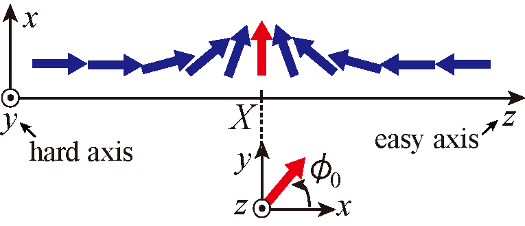
Figure 1: (Color online) The schematic figure of a DW formed by localized spins: X and $\phi_{0}$ are the displacement and the rotating angle of DW, respectively.

The character of DW motion becomes qualitatively different depending on which mechanism is dominant. So far, extensive theoretical studies [8, 11, 9, 10, 12, 13, 14] have shown that the “spin transfer” is the dominant mechanism for the DW motion in the experimental situations. Actually, many experimental results have been explained in this mechanism. [15, 16, 17, 18, 19]. On the other hand, the relevance of “momentum transfer” has been also reported in some experiments [20, 21]. The dynamics of thin DW also draws attention[22], in which more careful treatment is needed for the effect of non-adiabaticity of conduction electrons, i.e., the effect of “momentum transfer.”

Most of the theoretical studies have implicitly assumed that the conduction electrons obey a static distribution function slightly off the equilibrium state. Under such assumption, the non-adiabaticity of conduction electrons is not correctly taken into account. In particular, it is expected that the effect of “momentum transfer” is underestimated. Therefore, in this paper, we will treat the dynamics of conduction electrons and a DW on an equal footing, and discuss how the DW motion is affected by the strong non-adiabaticity of the conduction electron system.

Our model consists of a one-dimensional electron system under an electric field, which is coupled to a classical localized spin system,

$$\begin{split}\mathcal{H}(t)&=-t_{\mathrm{c}}\sum_{i,\sigma}[\mathrm{e}^{\mathrm{i}\Phi(t)}c_{i+1\sigma}^{\dagger}c_{i\sigma}+\mathrm{h.c.}]\\ &\quad-J_{\mathrm{sd}}\sum_{i,\sigma,\sigma^{\prime}}\boldsymbol{S}_{i}(t)\cdot c_{i\sigma}^{\dagger}\boldsymbol{\sigma}_{\sigma\sigma^{\prime}}c_{i\sigma^{\prime}}.\end{split}$$ (1)

Here, $c_{i\sigma}$($c_{i\sigma}^{\dagger}$) is an annihilation (creation) operator of the conduction electron at the $i$th site and spin $\sigma$ under the periodic boundary condition, $c_{i+N\sigma}=c_{i\sigma}$. $\boldsymbol{S}_{i}(t)$ denotes classical localized spins at the sites $i$, which constitute DWs with an easy z-axis and a hard y-axis. The electric field is applied via a time-dependent AB flux, $\Phi(t)$. In order to apply a direct electric field, we set $\Phi(t)=\frac{eV}{\hbar N}t$, where $V$ is the voltage drop in the circuit.

We study the dynamics of state vector of conduction electrons, $\left|\Psi(t)\right\rangle$, and the localized spins, $\boldsymbol{S}_{i}(t)$, simultaneously. $\left|\Psi(t)\right\rangle$ is determined by the time-dependent Schrödinger equation, $\mathrm{i}\hbar\frac{d}{dt}\left|\Psi(t)\right\rangle=\mathcal{H}(t)\left|\Psi(t)\right\rangle$. At the same time, we determine $\boldsymbol{S}_{i}(t)$ by solving the semiclassical Landau-Lifshitz-Gilbert (LLG) equations,

$$\dot{\boldsymbol{S}_{i}}=\boldsymbol{H}_{\mathrm{eff}i}\times\boldsymbol{S}_{i}-\alpha(\boldsymbol{S}_{i}/S)\times\dot{\boldsymbol{S}_{i}}.$$ (2)

The first term of eq. (2) represents the torque which leads to the precessional motion of the localized spin around the effective magnetic field, $\boldsymbol{H}_{\mathrm{eff}i}$. The second term corresponds to the Gilbert damping, which is essential to the relaxation of $\boldsymbol{S}_{i}$ parallel to $-\boldsymbol{H}_{\mathrm{eff}i}$. Here,

$$\begin{split}\boldsymbol{H}_{\mathrm{eff}i}&=-J(\boldsymbol{S}_{i-1}+\boldsymbol{S}_{i+1})-KS_{iz}\boldsymbol{e}_{z}\\ &\quad+K_{\perp}S_{iy}\boldsymbol{e}_{y}-J_{\mathrm{sd}}\left\langle\boldsymbol{\sigma_{i}}\right\rangle,\end{split}$$ (3)

with the exchange coupling between localized spins $J$, the easy-axis anisotropy $K$, the hard-axis anisotropy $K_{\perp}$, and the electron spin $\left\langle\boldsymbol{\sigma}_{i}(t)\right\rangle$ $=\left\langle\Psi(t)\right|\sum_{\sigma,\sigma^{\prime}}c_{i\sigma}^{\dagger}\boldsymbol{\sigma}_{\sigma\sigma^{\prime}}c_{i\sigma^{\prime}}\left|\Psi(t)\right\rangle$ at the $i$th site.

In order to solve the time-dependent Schrödinger equation numerically, we use the Crank-Nicholson’s method [23], $\left|\Psi(t+\varDelta t)\right\rangle$ $=\exp[-\frac{\mathrm{i}}{\hbar}\int_{t}^{t+\varDelta t}\mathcal{H}(t^{\prime})dt^{\prime}]\left|\Psi(t)\right\rangle$ $\simeq\frac{1-(\mathrm{i}/\hbar)\mathcal{H}(t+\varDelta t/2)\varDelta t/2}{1+(\mathrm{i}/\hbar)\mathcal{H}(t+\varDelta t/2)\varDelta t/2}\left|\Psi(t)\right\rangle$, which ensures the norm conservation of the state vector. For the LLG equations, we use the implicit fourth-order Runge-Kutta method.

We set the initial configuration ($t=0$) of the localized spins to be the static solution of the LLG equations, eq. (2), with two DWs: $\boldsymbol{S}_{i}(0)$ $=S\{1/\cosh[\frac{i_{c1}(0)-i}{W}],0,\tanh[\frac{i_{c1}(0)-i}{W}]\}$ for the sites $1\leq i$ $\leq N/2$, and $\boldsymbol{S}_{i}(0)=$ $[-S_{i-N/2x}(0),S_{i-N/2y}(0),-S_{i-N/2z}(0)]$ for $N/2+1\leq i\leq N$. Here, $i_{c1}(0)=(N+2)/4$ is the initial coordinate of the first DW center, and $W$ is the width of the DWs. Note that an even number of DWs are required for smooth connection at the boundary because of the periodic boundary condition. Since the relation $\boldsymbol{S}_{i+N/2}(t)=[-S_{ix}(t),S_{iy}(t),-S_{iz}(t)]$ holds within the simulation time, we only focus on the dynamics of the first DW. We assume the initial state vector, $\left|\Psi(0)\right\rangle$, to be the ground state of Hamiltonian, eq. (1), with the initial configuration, $\boldsymbol{S}_{i}(0)$.

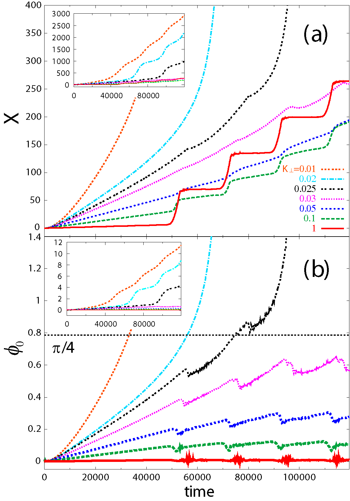
Figure 2: (Color online) The time dependence of (a)the displacement $X$, and (b)the rotating angle $\phi_{0}$ of the DW for several values of the hard-axis anisotropy $K_{\perp}$. The horizontal line of (b) corresponds to $\phi_{0}=\pi/4$. The scale of the longitudinal axis is expanded in the insets of (a) and (b).

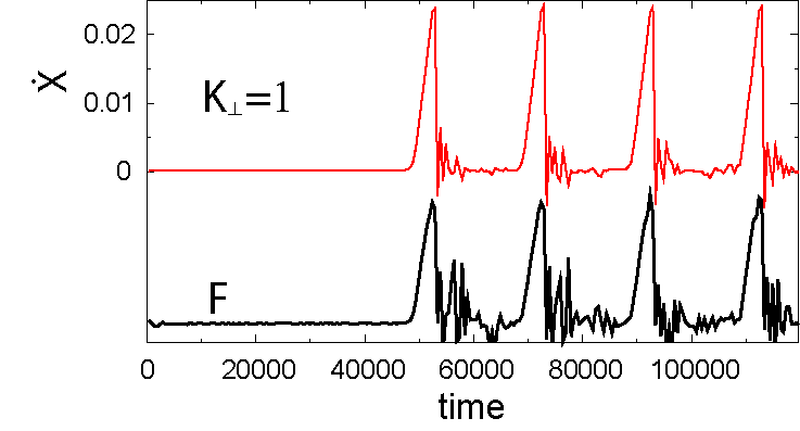
Figure 3: (Color online) The time dependence of the velocity, $\dot{X}$, and the force exerted by the electrons, $F$, for $K_{\perp}=1$. The amplitude of $F$ is plotted in arbitrary unit.

In order to characterize the DW motion, we define the displacement of DW center, $X(t)$, and the rotating angle of the localized spins in the DW center around z-axis, $\phi_{0}(t)$, as shown in Fig. 1. We will calculate the z-component of spin torque, $\tau_{z}(t)=J_{\mathrm{sd}}\sum_{i\in\mathrm{1stDW}}[\boldsymbol{S}_{i}(t)\times\left\langle\boldsymbol{\sigma_{i}}(t)\right\rangle]_{z}$. Since the first term in the right-hand side of eq. (2) involves the term proportional to $\tau_{z}(t)$, $\dot{S}_{iz}$ increases with $\tau_{z}(t)$. This means that $\tau_{z}(t)$ transfers z-axis angular momentum from conduction electrons to localized spins, and is essential to the “spin transfer” mechanism. We also calculate the force, $F(t)=-J_{\mathrm{sd}}\sum_{i\in\mathrm{1stDW}}\nabla\boldsymbol{S}_{i}(t)\cdot\left\langle\boldsymbol{\sigma_{i}}(t)\right\rangle$, which is the time variation of the momentum passed from the electron system to the localized spin system. Note that only if the DW has mass, $F(t)$ can be identified as a ‘real’ force exerted by the conduction electrons on the DW and is relevant to the “momentum transfer” mechanism. As shown below and derived in Ref. [tatara1], both $\tau_{z}(t)$ and $F(t)$ determine the dynamics of DW. In the following, we assume that $t_{\mathrm{c}}$ and $\hbar/t_{\mathrm{c}}$ are the units of energy and time, respectively, and that $\hbar=e=S=1$.

Here, we will show our results. The time evolution of $X(t)$ and $\phi_{0}(t)$ are shown in Figs. 2(a) and 2(b), respectively, for several values of $K_{\perp}$. We set $N=60$, $W=5$, $J=2.59$, $K=0.1$, $\alpha=0.02$, $J_{\mathrm{sd}}=0.3$, $V=\pi\times 10^{-4}$, and the electron density $n=12/N=0.2$. As shown in Figs. 2(a) and 2(b), the DW motion qualitatively changes, depending on the value of $K_{\perp}$.

Firstly, for small values of $K_{\perp}$ ($K_{\perp}=$ 0.01, 0.02, 0.025), $X(t)$ and $\phi_{0}(t)$ increase smoothly with $t$ as shown in the insets of Fig. 2. The constant increase of $\phi_{0}(t)$ is caused by the spin torque $\tau_{z}(t)$ with the help of Gilbert damping[24]. This streaming motion of the DW accompanied by the continuous increase of $\phi_{0}(t)$ means dominance of the “spin transfer” mechanism[8].

Secondly, for large values of $K_{\perp}$ ($K_{\perp}=$ 0.03, 0.05, 0.1, 1), step-like increase of $X(t)$ with $t$ is observed in Fig. 2(a). In this case, the rotating angle $\phi_{0}(t)$ is saturated at a finite value in a longer time scale in contrast to the case of smaller $K_{\perp}$. We plot the velocity $\dot{X}(t)$ and the force $F(t)$ for $K_{\perp}=1$ in Fig. 3. Remarkably, $\dot{X}(t)$ and $F(t)$ show peaks at the same time. This perfect correspondence clearly shows that the DW motion is driven by the force given by conduction electrons, i.e., the “momentum transfer” is the dominant driving mechanism in this region. We will later discuss the microscopic origin of the periodic peak structure of $F(t)$.

Here, we discuss the origin of crossover in driving mechanism between “spin transfer” and “momentum transfer.” The crossover results from the competition between the spin torque $\tau_{z}(t)$ and the hard-axis anisotropy $K_{\perp}$. $K_{\perp}$ tends to fix $\phi_{0}(t)\simeq 0$, while $\tau_{z}(t)$ increases $\phi_{0}(t)$ as we mentioned in the footnote [torqueeffect]. The origin of the crossover behavior can be interpreted using the effective equations of motion for $X(t)$ and $\phi_{0}(t)$,[8]

$$2(-\dot{\phi}_{0}+\alpha\dot{X}/W)=F,$$ (4)

$$2(\dot{X}+\alpha W\dot{\phi}_{0})=\tau_{z}-K_{\perp}W\sin 2\phi_{0},$$ (5)

where irrelevant coefficients are omitted. For $\tau_{z}(t)>K_{\perp}W$, since the right-hand side of eq. (5) is always finite, constant supply of the spin torque $\tau_{z}(t)\gg\alpha WF(t)$ keeps both $X(t)$ and $\phi_{0}(t)\sim\alpha X(t)/W$ increasing. This is why the DW motion for smaller $K_{\perp}$ is driven by the “spin transfer” (the insets in Fig. 2). In contrast, for $\tau_{z}(t)<K_{\perp}W$, the effect of the spin torque is canceled by the contribution of large $K_{\perp}$, and then $\phi_{0}(t)$ is saturated at the angle $\phi_{\mathrm{s}}=\frac{1}{2}\sin^{-1}\bigl{(}\frac{\tau_{z}}{K_{\perp}W}\bigr{)}(<\pi/4)$ in a longer time scale ($K_{\perp}\geq 0.03$ in Fig. 2(b)). This is the so-called intrinsic pinning effect for the “spin transfer” mechanism. In the case of $\tau_{z}(t)\ll K_{\perp}W$, since $\phi_{0}(t)\ll\pi/4$ and mass of the DW is well-defined as $M_{\mathrm{DW}}=\frac{2(1+\alpha^{2})}{K_{\perp}W}$, the “momentum transfer” from the conduction electrons becomes relevant to the DW motion.

With $\tau_{z}(t)\ll K_{\perp}W$ in mind, substituting $\phi_{0}(t)=\phi_{\mathrm{s}}+\delta\phi(t)$ into eqs. (4) and (5), we obtain the equations, $2(-\delta\dot{\phi}+\alpha\dot{X}/W)=F$, and $\dot{X}+\alpha W\delta\dot{\phi}=-K_{\perp}W\delta\phi$. The solutions are estimated as $\delta\dot{\phi}(t)=-\frac{1-c}{2(1+\alpha^{2})}F(t)$ and $\dot{X}(t)=\frac{W(c+\alpha^{2})}{2\alpha(1+\alpha^{2})}F(t)$, including a numerical factor, $0<c<1$. [25] In our calculation for $K_{\perp}=1$, $c\sim 0.95$ is obtained by numerically averaging the ratio of $\dot{X}(t)$ and $F(t)$ over the interval: $4\times 10^{4}<t<1.2\times 10^{5}$. Since $\alpha$ is small in general, the contribution of the force to the DW motion is remarkably enhanced, being inversely proportional to $\alpha$.[26] The fluctuation of $\phi_{0}(t)$ around the saturation angle $\phi_{\mathrm{s}}$ is crucial for the enhancement of the DW motion: $\dot{X}\propto\alpha^{-1}$.

Our calculation shows the absence of the perfect intrinsic pinning in a large $K_{\perp}$ region. While $\phi_{0}(t)$ is saturated for $K_{\perp}\geq 0.03$, the DW still shows a step-like motion. Absence of the intrinsic pinning has also been reported in the numerical study of ref. [ohe]. However, they attribute the origin of DW motion to the non-local deformation of localized spins, which is different from our results. In our calculation, deformation of localized spins is negligible.

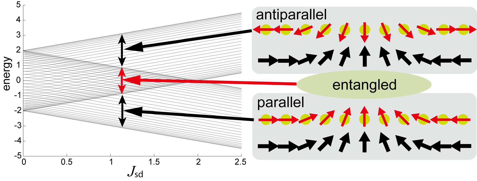
Figure 4: (Color online) One-particle energy levels $\{E_{i}(0)\}$ for various $J_{\mathrm{sd}}$ values. The energy levels split into two bands. For $J_{\mathrm{sd}}\lesssim\Omega/2$, the two bands overlap at $|E_{i}(0)|<-J_{\mathrm{sd}}+\Omega/2$ where spin and momentum degrees of freedom are entangled, and a complicated energy level structure is formed.

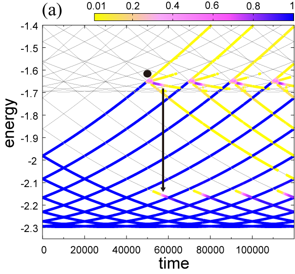
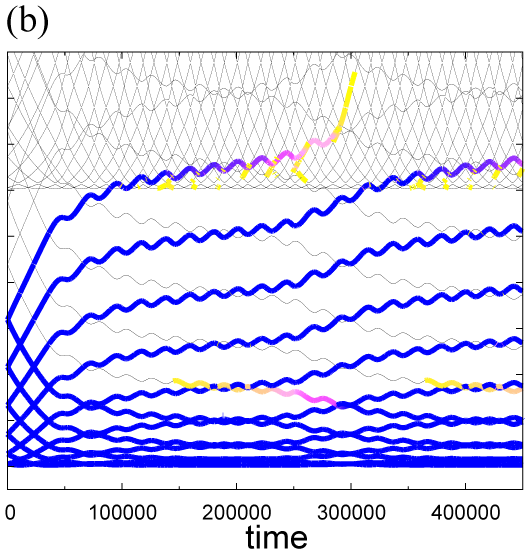
Figure 5: (Color online) The time dependence of the one-particle energy levels $\{E_{i}(t)\}$ (thin lines) and the one-particle distribution functions $\{|\left\langle\xi_{i}(t)|\Psi(t)\right\rangle|^{2}\}$ (color plots) of the electron system for $K_{\perp}=$ (a) $1$ and (b) $0.01$. Note that the time scale in (b) is much larger than that in (a). The color of the thick lines represents the occupation probability of each level. The dot and the arrow in (a) denote an elastic backscattering and an inelastic scattering,[29] respectively.

In order to understand the periodic step-like motion of the DW from a microscopic point of view, we will study the dynamics of electron state vector, $\left|\Psi(t)\right\rangle$. Before studying the dynamics, let us look at the one-particle energy levels at $t=0$, i.e., when there is a stationary DW. Figure 4 shows the energy levels $\{E_{i}(0)\}$ of the Hamiltonian $\mathcal{H}(t)$ (eq. (1)) at $t=0$ for various values of $J_{\mathrm{sd}}$. At $J_{\mathrm{sd}}=0$, the energy levels are simply those of one-dimensional tight-binding chain with a band width, $\Omega=4$. Each level is at least four-fold degenerate in terms of the reversal of momentum and spin. With increasing $J_{\mathrm{sd}}$, the spin degeneracy is lifted, and the energy levels gradually split into two bands. The lower (higher) band, $-(+)J_{\mathrm{sd}}-\Omega/2<E_{i}(0)<-(+)J_{\mathrm{sd}}+\Omega/2$, is composed of the states where the spins of conduction electrons are aligned parallel (antiparallel) to the localized spins. For not too large $J_{\mathrm{sd}}$ ($J_{\mathrm{sd}}\lesssim\Omega/2$), the two bands have an overlapping region, $|E_{i}(0)|<-J_{\mathrm{sd}}+\Omega/2$. Within each band, levels are labeled with different momentum except for the overlapping region, where neither spin nor momentum serve as a good quantum number, i.e., the eigenstates are composed of entangled spin and momentum degrees of freedom. This “entangled” energy range will play an important role in the dynamics in the larger $K_{\perp}$ region, as we will show below.

To characterize the dynamics of $\left|\Psi(t)\right\rangle$, we diagonalize the Hamiltonian $\mathcal{H}(t)$ (eq. (1)) at each $t$, and obtain the eigenvalues $\{E_{i}(t)\}$ and eigenvectors $\{\left|\xi_{i}(t)\right\rangle\}$. We then plot the time evolution of one-particle energy levels $\{E_{i}(t)\}$ and distribution functions $\{|\left\langle\xi_{i}(t)|\Psi(t)\right\rangle|^{2}\}$ in Fig. 5, corresponding to the DW motions for $K_{\perp}=1$ and $K_{\perp}=0.01$. First, let us discuss the case of large $K_{\perp}$ (Fig. 5 (a)). In general, the time dependence of $\{E_{i}(t)\}$ comes from the AB flux, $\Phi(t)$, and the localized spins, $\boldsymbol{S}_{i}(t)$ in eq. (1). For $K_{\perp}=1$, the dynamics of $\{E_{i}(t)\}$ is mostly determined by $\Phi(t)$, since $\boldsymbol{S}_{i}(t)$ is constant except for the moments at which $\dot{X}(t)$ shows peaks (Fig. 3). $\Phi(t)$ accelerates the electron momentum with an acceleration rate: $dk/dt\sim V/N$. As to the distribution functions, only the states below the Fermi energy ($\varepsilon_{\mathrm{F}0}\sim-1.98$) are occupied at $t=0$. Therefore, for small $t$, all the occupied states are within the range $E_{i}(t)<J_{\mathrm{sd}}-\Omega/2$. In this energy range, each state continues to be accelerated without scattering, since momentum serves as a good quantum number [27]. On the other hand, when $E_{i}(t)$ enter the “entangled” energy range, $|E_{i}(t)|<-J_{\mathrm{sd}}+\Omega/2$, an elastic backscattering with spin flip occurs, and as a result, the DW acquires a recoil momentum[28]. The backscattering causes rapid oscillation of the localized spins (see the oscillating behavior of $\dot{X}(t)$ just after the peaks in Fig. 3), which leads to the dissipation (arrow in Fig. 5(a)).[29]

With the difference of momentum between the successive energy levels at $t=0$, $\delta k\sim 2\pi/N$, the interval between the backscatterings $\delta t$ is estimated as $\delta t\sim\delta k/(dk/dt)\sim 2\pi/V$. Using $V=\pi\times 10^{-4}$, we have $\delta t=2\times 10^{4}$, consistent with Fig. 5(a), where backscatterings happen at time $t_{\mathrm{eb}}\sim 5\times 10^{4},7\times 10^{4},9\times 10^{4}\cdots$. Remarkably, the backscatterings occur exactly at the moments at which $F(t)$ has peaks (Fig. 3). This correspondence shows that the backscatterings in the “entangled” energy range is the origin of the periodic step-like DW motion. Actually, the most part of DW shift $\varDelta X_{\mathrm{ave}}\sim 65$ (Fig. 2(a)), which is a time-averaged value of $X$ between $t_{\mathrm{eb}}-\delta t/2<t<t_{\mathrm{eb}}+\delta t/2$, can be explained by the “momentum transfer” at the elastic backscattering, $\varDelta X_{\mathrm{eb}}=\frac{W(c+\alpha^{2})}{2\alpha(1+\alpha^{2})}\varDelta k\sim 62$, where $\varDelta k\sim 10\delta k/2$ is a momentum shift per DW at $t_{\mathrm{eb}}$ estimated in Fig. 5(a). It is tempting to associate the step-like DW motion with the stick-slip motion [30]: “stick” caused by the pinning due to the hard-axis anisotropy $K_{\perp}$, and “slip” caused by backscatterings of the electrons. The stick-slip motion vanishes, if the lifetime of conduction electrons is shorter than $2\pi/V$. However, it may be observed in a clean mesoscopic sample.

Next, we discuss the case of small $K_{\perp}$, i.e., $K_{\perp}=0.01$ (Fig. 5(b)). The qualitative feature of level dynamics is distinct from that for $K_{\perp}=1$. As soon as the electric field is applied at $t=0$, the energy levels of the lower band start to reconstruct themselves so that each level has almost time-independent energy, except for small oscillations. As a result, the system falls into a nonequilibrium steady state, where the inter-level transition rarely happens. The distribution function of the system can be well approximated by a shifted Fermi distribution function, with the total momentum proportional to the applied electric field[8, 13].

In summary, we have studied the current-induced dynamics of a DW by solving the time-dependent Schrödinger equation and the LLG equations simultaneously for a one-dimensional tight-binding chain coupled to a localized spin system. We observe two types of DW motions depending on the hard-axis anisotropy of the localized spin system, $K_{\perp}$. For smaller $K_{\perp}$, the DW shows a streaming motion driven by the spin transfer. In contrast, for larger $K_{\perp}$, we obtain a stick-slip motion driven by the momentum transfer. To our knowledge, our work provides the first numerical realization of the crossover between the two regimes. We have also interpreted the qualitative features of the DW motion in both regimes, in terms of the dynamics of one-particle energy levels and distribution functions. In particular, we found that the stick-slip motion at larger $K_{\perp}$ comes from the backscatterings in the “entangled” energy range. Our results indicate that the DW motion at larger $K_{\perp}$ is influenced by the microscopic energy level structure, which has been neglected in most of the previous works. The competition between the stick-slip motion and an extrinsic pinning or impurities is an interesting future problem.[19, 20, 21, 22]

The authors thank I. Maruyama and S. Kasai for fruitful discussions. This work was supported by the Next Generation Super Computing Project, Nanoscience Program, MEXT, Japan. and also supported by GCOE for Phys. Sci. Frontier, MEXT, Japan.

References

- [1] A. J. Heeger, S. Kivelson, J. R. Schrieffer, and W.-P. Su: Rev. Mod. Phys. 60 (1988) 781.
- [2] M. Tinkham: Introduction to Superconductivity (McGraw-Hill, New York, 1996) 2nd Ed.
- [3] G. Tatara, H. Kohno and J. Shibata: J. Phys. Soc. Jpn. 77 (2008) 031003.
- [4] L. Berger: Phys. Rev. B 54 (1996) 9353.
- [5] J. C. Slonczewski: J. Magn. Magn. Mater. 159 (1996) L1.
- [6] S. S. P. Parkin, M. Hayashi and L. Thomas: Science 320 (2008) 190.
- [7] L. Berger: J. Appl. Phys. 55 (1984) 1954; J. Appl. Phys. 71 (1992) 2721.
- [8] G. Tatara and H. Kohno: Phys. Rev. Lett. 92 (2004) 086601.
- [9] A. Thiaville, Y. Nakatani, J. Mittat, and N. Vemier: J. Appl. Phys. 95 (2004) 7049.
- [10] Z. Li and S. Zhang: Phys. Rev. B 70 (2004) 024417.
- [11] S. E. Barnes and S. Maekawa : Phys. Rev. Lett. 95 (2005) 107204.
- [12] J.-I. Ohe and B. Kramer : Phys. Rev. Lett. 96 (2006) 027204.
- [13] J. Xiao, A. Zangwill and M. D. Stiles: Phys. Rev. B 73 (2006) 054428.
- [14] A. K. Nguyen, H. J. Skadsem and A. Brataas: Phys. Rev. Lett. 98 (2007) 146602.
- [15] A. Yamaguchi, T. Ono, S. Nasu, K. Miyake, K. Mibu and T. Shinjo: Phys. Rev. Lett. 92 (2004) 077205; Phys. Rev. Lett. 96 (2006) 179904.
- [16] M. Yamanouchi, D. Chiba, F. Matsukura and H. Ohno: Nature 428 (2004) 539.
- [17] M. Kläui, C. A. F. Vaz, J.A.C. Bland, W. Wernsdorfer, G. Faini, E. Cambril, L. J. Heyderman, F. Nolting and U. Rüdiger: Phys. Rev. Lett. 94 (2005) 106601.
- [18] L. Thomas, M. Hayashi, X. Jiang, R. Moriya, C. Rettner and S. S. P. Parkin: Science 315 (2007) 1553.
- [19] M. Yamanouchi, J. Ieda, F. Matsukura, S. E. Barnes, S. Maekawa and H. Ohno: Science 317 (2007) 1726.
- [20] E. Saitoh, H. Miyajima, T. Yamaoka and G. Tatara: Nature 432 (2004) 203.
- [21] M. Hayashi, L. Thomas, C. Rettner, R. Moriya, Y. B. Bazaliy and S. S. P. Parkin: Phys. Rev. Lett. 98 (2007) 037204.
- [22] M. Feigenson, J. W. Reiner, and L. Klein: Phys. Rev. Lett. 98 (2007) 247204.
- [23] W. H. Press, S. A. Teukolsky, W. T. Vetterling and B. P. Flannery: Numerical Recipes in C (Cambridge Univ. Press, Cambridge, 1997) 2nd ed., Chap. 19. Sec. 2.
- [24] tends to relax parallel to due to the Gilbert damping. Since the electron spin term is involved in (eq. (3)), is attracted parallel to . This is why increases .
- [25] The numerical factor is defined by the relation: , where the relaxation time due to the Gilbert damping, .
- [26] G. Tatara, T. Takayama, H. Kohno, J. Shibata, Y. Nakatani and H. Fukuyama: J. Phys. Soc. Jpn. 75 (2006) 046708.
- [27] While the translational symmetry is broken due to DW, its effect is negligible except for the “entangled” region, then momentum can be regarded as a good quantum number.
- [28] Even in the entangled region, the backscattering does not occur at every “crossing” of energy levels. For some crossings, the degree of level repulsion is small.
- [29] The energy of localized spin system varies as with . Firstly, the rapid oscillation of the localized spins (large ) transfers the energy of electron system to the localized spin system, through the first term of this equation. After that, The energy of localized spins is dissipated due to the second term (Gilbert damping), then the state of the total system is restored to the state before the backscattering.
- [30] B. N. J. Persson and E. Tosatti: Physics of Sliding Friction (Kluwer, Dordrecht, 1996).