Orbital Evolution of a Particle Interacting with a Single Planet in a Protoplanetary Disk

Abstract

We investigate the motion of a particle around a low mass planet embedded in a non-turbulent gaseous disk. We take into account the effect of the gas structure that is modified by the gravitational interaction between the planet. We derive an analytic formula that describes the change of the semi-major axis of the particle due to the encounter with the planet using local approximation in distant encounter regime. Our final formula includes the effects of steady, axisymmetric radial gas flow, the global gas pressure gradient in the disk, planet gravity, and the structure of the gas flow modified by the planet’s gravity. We compare the analytic results with numerical calculations, and indicate that our formula well describes the secular evolution of the dust particles’ semi-major axes well, especially for small particles with large drag coefficient. We discuss the conditions for dust gap opening around a low mass planet and radial distribution of dust particles. Our formula may provide a useful tool for calculating radial distribution of particles in a disk around the planet.

1 Introduction

The motion of small particles in a gas disk has been investigated in detail since this is essential for planet formation theory. In a number of work, an axisymmetric gas disk is assumed and the effects of the structure of the gas disk on particle orbit are investigated, neglecting the effects of planet’s gravitational force (Adachi et al. 1976, Weidenschilling 1977). Their results show that particles with stopping timescale of the order of Kepler timescale migrate towards the central star rapidly, thereby imposing a serious barrier on the formation of planetesimals.

Although this poses a serious question on the formation of planetesimals, there is another aspect of this fact in the formation of gas giant core. Gas giant core should reach the critical mass to accrete nearby gas rapidly (Mizuno et al. 1978), and its formation timescale seems to be very long (Pollack et al. 1993). If the global pressure gradient exerted on the gas disk will force the particles to migrate towards the central star, the particles at outer disk may reach the orbit of an already formed core and may accrete onto it. Kary et al. (1993) have shown that this process seems to be possible but most of the particles may miss the planet since they migrate very rapidly. Their discussion is based on the three-body problem including the effect of axisymmetric gas disk.

The assumption of axisymmetric gas disk is a simplification in order to make the calculation tractable. The planet gravitationally interacts with the gas disk and changes the structure of the disk around it, producing the spiral density wave (see e.g., Goldreich and Tremaine 1979). Only recently does appear the investigation of particle motion around the planet embedded in a gas disk, which fully takes into account the structure around the planet (Paardekooper and Mellema 2004, 2006, Paardekooper 2007, Fouchet et al. 2007, Lyra et al. 2008). For instance, Paardekooper and Mellema (2004, 2006) and Paardekooper (2007) numerically calculated the particle motion around a high mass planet in the presence of a gas disk and discussed the accretion of the particles onto the planet and the formation of gap of particles of different size. They concluded that minimum mass of the planet that opens up a dust gap was $0.05M_{J}$, thereby indicating the possibility of detecting a low mass planet by future observations by observing a dust gap.

Many of such works involve numerical studies on particle motion. In this paper, we present an analytic investigation of the motion of particles around a low mass planet embedded in a gas disk, taking into account of the structure around the planet. This is the full analytic solution of a particle motion around the planet in which the structure of the gas disk is fully taken into account. We consider a vertically averaged disk and perform two-dimensional analysis for simplicity. We use the results of (quasi-)linear calculation of the gas structure around the planet and calculate the distant encounter between a particle and a planet embedded in a gaseous disk. We derive a formula which describes the secular change of the semi-major axis of the particle caused by the encounter with the planet using Hill’s equations. It is not possible to describe the resonant capture discussed by Weidenschilling and Davis (1985) or Kary et al. (1993); however, we take into account the structure of the gaseous disk that is modified by the planet, which is not considered in most of the previous analytic works. Our paper is complementary with previous numerical studies in two respects. Firstly, our analysis is focused on low mass planet, and secondly, our treatment is analytic. It is challenging to follow numerically the motion of dust particles embedded in a gas disk for long timescale (e.g., $10^{5}$ Kepler time), solving gas and the motion of dust simultaneously. Therefore, analytic treatment may be necessary in order to understand the secular motion of dust particles. Moreover, basic physical processes in the problem become clear by analytic treatment.

The plan of this paper is as follows. In Section 2, we show analytic treatment of the problem and derive the formula for the evolution of semi-major axis, equation (70). This formula includes the effects of global pressure gradient of gas disk, steady, axisymmetric mass accretion flow of the gas, gravitational force from the planet, and the gas velocity structure modified by the planet. We then compare our results with numerical calculations in Sections 3 and 4, and the limitations of our analytic approach are discussed. In Section 5, we discuss the conditions for dust gap formation and long-term behavior of dust particles whose orbits are close to an embedded planet. Section 6 is for summary and future prospects.

We expect that our results, equation (70), can be used as a tool for estimate radial motion of the particle in a disk around the planet, since this is written in an analytic form. It may be possible to calculate the radial distribution of particles of various sizes using this formula and derive, for example, the opacity of the disk. We recommend readers who need only the final results of the particle motion just to refer equation (70) directly and go to Section 5.2 where we demonstrate the calculation of radial dust distribution around a planet.

Before proceeding to the details of calculations, we note that there are two relevant length scales in the problem at hand: pressure scale height $H$ of the gas disk and Hill’s radius of the planet, $r_{\rm H}$. Pressure scale height is an important quantity for the structure of gas modified by the gravitational force of the planet, while Hill’s radius is important for the orbit of particles. Pressure scale height that is given by sound speed of the gas $c$ divided by Keplerian angular velocity and Hill’s radius of the planet are related by

$${\displaystyle\frac{r_{\rm H}}{H}}\sim{\displaystyle\frac{r_{\rm p}}{H}}\left({\displaystyle\frac{M_{\rm p}}{M_{\rm c}}}\right)^{1/3}=\left({\displaystyle\frac{GM_{\rm p}}{Hc^{2}}}\right)^{1/3},$$ (1)

where $r_{\rm p}$ is the semi-major axis of the planet, $M_{\rm p}$ is the mass of the planet, and $M_{\rm c}$ is the mass of the central star. For low mass planets considered in this paper, $r_{\rm H}/H$ is smaller than unity.

2 Analytic Consideration

In this section, we analytically investigate the particle motion under the influence of gravitational force by the protoplanet and gas drag using local approximation. We show that particles with friction time of the order Kepler time will migrate towards the planet because of the gas drag, although gravitational scattering tends to repel the particle from the planet. This mechanism is different from the inward migration of dust particles caused by the velocity difference between the gas and dust [see e.g., Adachi et al. (1976) or Weidenschilling (1977)]. We also derive the effects of the modification of gas velocity due to the gravitational force of the planet.

2.1 Basic Equations

We use Hill’s approximation to investigate the encounter between the particle and the planet. We consider the motion only in $(x,y)$ plane where $x$ is in radial direction and $y$ is in the azimuthal direction. We assume the planet is fixed at the origin $(x,y)=(0,0)$ in this coordinate and neglect the mass of the particle. We write the velocity of the gas $\mbox{\boldmath$v$}_{\rm g}$ by

$$\mbox{\boldmath$v$}_{\rm g}=-{\displaystyle\frac{3}{2}}\Omega_{\rm p}x\mbox{\boldmath$e$}_{y}+\delta\mbox{\boldmath$v$}_{\rm g},$$ (2)

where $\Omega_{\rm p}$ is the Keplerian angular velocity of the planet and $\mbox{\boldmath$e$}_{y}$ is the unit vector in the $y$-direction. The first term represents the Keplerian motion around the central star and the second term $\delta\mbox{\boldmath$v$}_{\rm g}$ represents the deviation from this motion, which, for instance, may be caused by the global pressure gradient of the disk.

The equations of motion of the particle are

$$\ddot{x}-2\Omega_{\rm p}\dot{y}=3\Omega_{\rm p}^{2}x-\nu\dot{x}+F_{x}$$ (3)

$$\ddot{y}+2\Omega_{\rm p}\dot{x}=-\nu\left(\dot{y}+{\displaystyle\frac{3}{2}}\Omega_{\rm p}x\right)+F_{y}$$ (4)

where $\nu$ stands for the drag coefficient. The quantity $\nu$ is a reciprocal of the stopping time of a particle. Note that there are various notations for this parameter. In Weidenschilling (1977), stopping time is denoted by $t_{e}$ so $\nu$ in this paper is equal to $1/t_{e}$. In Adachi et al. (1976), stopping time corresponds to their $A$ times gas density times relative velocity. We write the sum of the force exerted by the planet and the part of the friction force caused by the non-Keplerian motion of the gas by $F$,

$$\mbox{\boldmath$F$}(x,y)=\nabla\frac{GM_{\rm p}}{\sqrt{x^{2}+y^{2}}}+\nu\delta\mbox{\boldmath$v$}_{\rm g}(x,y),$$ (5)

where $G$ is the gravitational constant and $M_{\rm p}$ denotes the mass of the planet.

We give a brief note on the relationship between the dust size and drag coefficient. In this paper, we use the constant drag coefficient $\nu$ for mathematical convenience. The dust size $d$ and the drag coefficient $\nu$ are related by $\nu\propto d^{-1}$ for Epstein law and $\nu\propto d^{-2}$ for Stokes law. Simple relationship between the dust size and drag coefficient may be given by

$${\displaystyle\frac{\nu}{\Omega_{\rm p}}}=\left\{\begin{array}[]{cc}10^{4}\left({\displaystyle\frac{\rho_{0}}{10^{-9}\mathrm{g/cm}^{3}}}\right)\left({\displaystyle\frac{d}{1\mathrm{cm}}}\right)^{-1}&{\displaystyle\frac{d}{1\mathrm{cm}}}<{\displaystyle\frac{10^{-9}\mathrm{g/cm}^{3}}{\rho_{0}}}\\[15.0pt] 10^{4}\left({\displaystyle\frac{d}{1\mathrm{cm}}}\right)^{-2}&{\displaystyle\frac{10^{-9}\mathrm{g/cm}^{3}}{\rho_{0}}}<{\displaystyle\frac{d}{1\mathrm{cm}}}\end{array}\right.$$ (8)

where $\rho_{0}$ is the background density and $d$ is the size of the particle. Figure 1 shows the relationship between dust size and drag coefficient given by this equation for $\rho_{0}=10^{-8}\mathrm{gcm}^{-3}$, $10^{-10}\mathrm{gcm}^{-3}$, and $10^{-12}\mathrm{gcm}^{-3}$.

The assumption of constant drag coefficient is not true for large bodies whose drag force is proportional to the square of the velocity difference. However, we expect that the results are qualitatively similar even for large bodies.

We neglect the effects of gravitational potential caused by gas disk. It is a good approximation for non-self-gravitating disk as shown in Section 2.6.

In the absence of the planet and the friction force, the particle motion is the Keplerian motion around the central star. In our setup, this is represented by four orbital elements $(b,h,k,y_{0})$,

$$x(t)=b+r_{\rm p}h\cos(\Omega_{\rm p}t)+r_{\rm p}k\sin(\Omega_{\rm p}t)$$ (9)

$$y(t)=y_{0}-{\displaystyle\frac{3}{2}}b\Omega_{\rm p}t-2r_{\rm p}h\sin(\Omega_{\rm p}t)+2r_{\rm p}k\cos(\Omega_{\rm p}t).$$ (10)

Physically, $b$ is the difference of orbital semi-major axis between the planet and the particle, $h$ and $k$ are quantities related to the orbital eccentricity, and $y_{0}$ is related to the initial azimuthal position of the particle.

We calculate the evolution of the orbital elements caused by the planet’s gravitational force and the friction due to the gas. The time evolution of the osculating elements is given by

$$\dot{b}=\nu r_{\rm p}\left[h\cos(\Omega_{\rm p}t)+k\sin(\Omega_{\rm p}t)\right]+{\displaystyle\frac{2}{\Omega_{\rm p}}}F_{y}$$ (11)

$$\dot{h}=-\nu h-{\displaystyle\frac{1}{r_{\rm p}\Omega_{\rm p}}}\left[F_{x}\sin(\Omega_{\rm p}t)+2F_{y}\cos(\Omega_{\rm p}t)\right]$$ (12)

$$\dot{k}=-\nu k+{\displaystyle\frac{1}{r_{\rm p}\Omega_{\rm p}}}\left[F_{x}\cos(\Omega_{\rm p}t)-2F_{y}\sin(\Omega_{\rm p}t)\right].$$ (13)

2.2 Change of Semi-Major Axis by Distant Encounter: General Treatment

We now solve equations (11)-(13). We assume that the particle is in circular orbit initially: $h(t=-\infty)=k(t=-\infty)=0$. We derive the change of orbital semi-major axis $\Delta b=b(t=\infty)-b(t=-\infty)$ by the encounter.

The formal solutions of equations (12) and (13) are given by

$$h(t)=-{\displaystyle\frac{1}{r_{\rm p}\Omega_{\rm p}}}\int_{0}^{\infty}due^{-\nu u}\left\{F_{x}(t-u)\sin[\Omega_{\rm p}(t-u)]+2F_{y}(t-u)\cos[\Omega_{\rm p}(t-u)]\right\}$$ (14)

$$k(t)={\displaystyle\frac{1}{r_{\rm p}\Omega_{\rm p}}}\int_{0}^{\infty}due^{-\nu u}\left\{F_{x}(t-u)\cos[\Omega_{\rm p}(t-u)]-2F_{y}(t-u)\sin[\Omega_{\rm p}(t-u)]\right\},$$ (15)

where $F_{x}(t)$ denotes $F_{x}(x(t),y(t))$ where $(x(t),y(t))$ is the location of the particle at time $t$ given by equations (9) and (10) and so for $F_{y}$. Substituting equations (14) and (15) into equation (11), we find

$$\Delta b \equiv\int_{-\infty}^{\infty}\dot{b}(t)dt$$ (16)

$$={\displaystyle\frac{\nu}{\Omega_{\rm p}}}\int_{-\infty}^{\infty}dt\int_{0}^{\infty}due^{-\nu u}\left\{F_{x}(t-u)\sin(\Omega_{\rm p}u)-2F_{y}(t-u)\cos(\Omega_{\rm p}u)\right\}$$

$$\ \ \ +{\displaystyle\frac{2}{\Omega_{\rm p}}}\int_{-\infty}^{\infty}dtF_{y}(t)$$

Changing the integration variable $t\to t-u$ in the first integral of the second line and using the formula

$$\int_{0}^{\infty}due^{-\nu u}\cos(\Omega_{\rm p}u)={\displaystyle\frac{\nu}{\nu^{2}+\Omega_{\rm p}^{2}}}$$ (17)

and

$$\int_{0}^{\infty}due^{-\nu u}\sin(\Omega_{\rm p}u)={\displaystyle\frac{\Omega_{\rm p}}{\nu^{2}+\Omega_{\rm p}^{2}}},$$ (18)

we find

$$\Delta b={\displaystyle\frac{\nu}{\nu^{2}+\Omega_{\rm p}^{2}}}\int_{-\infty}^{\infty}F_{x}(t)dt+2{\displaystyle\frac{\Omega_{\rm p}}{\nu^{2}+\Omega_{\rm p}^{2}}}\int_{-\infty}^{\infty}F_{y}(t)dt$$ (19)

This equation formally describes the amount of change of semi-major axis. We note that the integration with respect to $t$ must be performed along the particle’s trajectory. The force $F$ consists of two parts [see equation (5)]. One is the gravitational force of the planet and the other is the non-Keplerian motion of the gas velocity. We now see these effects separately.

2.3 Planet Encounter

First, we consider the change of the semi-major axis caused by the planet. We assume that the trajectory of the particle is close to circular orbit. We approximate $F_{x}$ by

$$F_{x}\sim-\mathrm{sgn}(b){\displaystyle\frac{GM_{\rm p}}{b^{2}}}{\displaystyle\frac{1}{(1+(9/4)\Omega_{\rm p}t^{2})^{3/2}}}.$$ (20)

With this approximation, we obtain

$$\int_{-\infty}^{\infty}F_{x}(t)dt=-\mathrm{sgn}(b){\displaystyle\frac{4GM_{\rm p}}{3b^{2}}}.$$ (21)

For the integration of $F_{y}$, we can use the well-known result of restricted three-body problem (see e.g., Goldreich & Tremaine 1980, Hénon & Petit 1986, or Hasegawa & Nakazawa 1990). The result is

$$\int_{-\infty}^{\infty}F_{y}(t)dt={\displaystyle\frac{64}{243}}{\displaystyle\frac{G^{2}M_{\rm p}^{2}}{b^{5}\Omega_{\rm p}^{3}}}\left[K_{1}\left({\displaystyle\frac{2}{3}}\right)+2K_{0}\left({\displaystyle\frac{2}{3}}\right)\right]^{2},$$ (22)

where $K_{0}$ and $K_{1}$ are modified Bessel function of zeroth and first order. The derivation of this equation is outlined in Appendix A.

Substituting equations (21) and (22) into equation (19), we obtain

$$\Delta b=-\mathrm{sgn}(b)4{\displaystyle\frac{r_{\rm H}^{3}}{b^{2}}}{\displaystyle\frac{\nu\Omega_{\rm p}}{\nu^{2}+\Omega_{\rm p}^{2}}}+\alpha{\displaystyle\frac{r_{\rm H}^{6}}{b^{5}}}{\displaystyle\frac{\Omega_{\rm p}^{2}}{\nu^{2}+\Omega_{\rm p}^{2}}},$$ (23)

where $r_{\rm H}$ is the Hill’s radius of the planet defined by

$$r_{\rm H}=\left({\displaystyle\frac{M_{\rm p}}{3M_{\ast}}}\right)^{1/3}r_{\rm p}$$ (24)

and $\alpha$ is a numerical factor

$$\alpha\equiv{\displaystyle\frac{128}{27}}\left[K_{1}\left({\displaystyle\frac{2}{3}}\right)+2K_{0}\left({\displaystyle\frac{2}{3}}\right)\right]^{2}=30.094$$ (25)

The second term of equation (23) represents the effect of gravitational scattering. The particle and the planet tends to repel each other by mutual gravitational interaction, which is a well-known result of restricted three-body problem. This effect remains when drag force vanishes ($\nu\to 0$). When there is no drag force, the gravitational interaction between the planet and the particle results in the excitation of eccentricity and the difference in semi-major axes of the two increases since Jacobi energy must be conserved in the absence of any dissipative force.

When friction force is large, gravitational scattering is ineffective since the gas drag enforces the particle to move with the fluid element. The first term of the equation (23) shows that the orbits of the planet and the particle tend to attract each other and this is most efficient when $\Omega_{\rm p}\sim\nu$. The intuitive explanation of this effect is as follows. When the particle feels the gravitational force of the planet, it is attracted towards the planet’s position at first. Then, when the gas drag is effective, the gas enforces the particle to stay at the Kepler orbit at the location where the particle is attracted, resulting in the attraction of the semi-major axes of the particle and the planet. If the drag force is taken into account, the semi-major axis difference between the planet and the particle can shrink since Jacobi energy is not necessarily conserved.

Since the attraction of the semi-major axes of the particle and the planet in the presence of drag force represented by the first term of equation (23) is proportional to $b^{-2}$ at large $b$, this overwhelms the effect of scattering represented by the second term, which is proportional to $b^{-5}$. Therefore, we conclude that particles far away from the planet are attracted towards the planet when the gas velocity equals Keplerian rotation velocity.

In the vicinity of the planet, it is expected that gravitational scattering is more effective since this effect increases as $b^{-5}$. The value of $b$ where these two effects are comparable is given by $\Delta b=0$, that is

$$|b|\sim 1.96\left({\displaystyle\frac{\Omega_{\rm p}}{\nu}}\right)^{1/3}r_{\rm H}.$$ (26)

This indicates that particles with $\nu>\Omega_{\rm p}$ may move towards the planet even in the absence of the global pressure gradient.

2.4 Non-Keplerian Rotation of Gas Disk due to Pressure Gradient

In this subsection, we consider the change of the semi-major axis caused by the effect of non-Keplerian rotation of the gas, which is due to the presence of global pressure gradient. The result of this section is already derived by previous studies such as Adachi et al. (1976) or Weidenschilling (1977), but we briefly show the results in this formulation for completeness.

We parameterize the degree of non-Keplerian rotation by $\eta$ and write the velocity difference $\delta\mbox{\boldmath$v$}_{\rm g}$ by

$$\delta\mbox{\boldmath$v$}_{\rm g}=\eta v_{\rm p}\mbox{\boldmath$e$}_{y}=\mathrm{const},$$ (27)

where $v_{\rm p}$ is the rotation velocity of the planet around the central star, $v_{\rm p}=r_{\rm p}\Omega_{\rm p}$. The parameter $\eta$ is non-dimensional and its magnitude is the order of the square of the disk aspect ratio. This is negative for the disk with negative pressure gradient.

Since $\delta\mbox{\boldmath$v$}_{\rm g}$ is constant, it is easy to integrate (19) to obtain

$$\Delta b=2\eta v_{\rm p}T{\displaystyle\frac{\nu\Omega_{\rm p}}{\nu^{2}+\Omega_{\rm p}^{2}}},$$ (28)

where $T$ is the time taken for the particle to cross the box. As is well-known, this effect is most efficient for the particle with $\nu\sim\Omega_{\rm p}$.

2.5 Steady Accretion Flow

In this subsection, we consider the change of the semi-major axis caused by the steady accretion (or deccretion) flow. This may be modeled by the constant axisymmetric radial velocity $\delta v_{x}$. We parameterize the radial velocity by non-dimensional factor $\zeta$ as follows,

$$\delta\mbox{\boldmath$v$}_{\rm g}=\zeta v_{\rm p}\mbox{\boldmath$e$}_{x}=\mathrm{const}.$$ (29)

The parameter $\zeta$ denotes the ratio between the radial flow velocity and the Kepler velocity. If the dissipation of the gaseous nebula is due to the gas accretion, the sign of $\zeta$ is negative and its magnitude is the order of $10^{-6}$, which is indicated from observation (see, e.g., Haisch et al. 2001). Drag force due to the gas is given by $\nu\delta\mbox{\boldmath$v$}_{\rm g}$ and therefore, using equation (19), we find

$$\Delta b=\zeta v_{\rm p}T{\displaystyle\frac{\nu^{2}}{\nu^{2}+\Omega_{\rm p}^{2}}}.$$ (30)

We note that the steady accretion flow effect is important for small particles, which have large drag coefficient $\nu$, since such particles move in the same way as the gas flow.

2.6 Non-Keplerian Rotation of Gas due to the Presence of the Planet

In this section, we consider the change of the orbital semi-major axis of the particle caused by the deviation of the gas velocity from Keplerian rotation velocity due to the presence of the planet. In this section, $\delta\mbox{\boldmath$v$}_{\rm g}$ is caused by the gravitational interaction between gas and the embedded planet, in contrast to the previous sections. We show that only axisymmetric structure of the disk causes the change of the semi-major axis of the particle.

In order to calculate the velocity perturbation caused by the planet, we solve vertically averaged Euler equations using local shearing-sheet approximation:

$${\displaystyle\frac{\partial\Sigma}{\partial t}}+\nabla\cdot(\Sigma\,\mbox{\boldmath$v$})=0,$$ (31)

$${\displaystyle\frac{\partial\mbox{\boldmath$v$}}{\partial t}}+(\mbox{\boldmath$v$}\cdot\nabla)\mbox{\boldmath$v$}=3\Omega_{\rm p}^{2}x\mbox{\boldmath$e$}_{x}-{\displaystyle\frac{c^{2}}{\Sigma}}\nabla\Sigma-\nabla\psi_{\rm p}-2\Omega_{\rm p}(\mbox{\boldmath$e$}_{z}\times\mbox{\boldmath$v$}),$$ (32)

where $\Sigma$ denotes the surface density, $v$ is the gas velocity, $c$ is the sound speed, and $\Omega_{\rm p}$ is the Keplerian angular velocity of the planet. We assume an isothermal disk, where $c$ is constant, for simplicity. The gravitational potential of the planet, $\psi_{\rm p}$ is given by

$$\psi_{\rm p}=-{\displaystyle\frac{GM_{\rm p}}{\sqrt{x^{2}+y^{2}+\epsilon^{2}}}},$$ (33)

where $\epsilon$ is the softening parameter. Taking the rotation of the equation of motion, we obtain the equation for vorticity,

$$\left({\displaystyle\frac{\partial}{\partial t}}+\mbox{\boldmath$v$}\cdot\nabla\right)\left[{\displaystyle\frac{1}{\Sigma}}\left\{{\displaystyle\frac{\partial v_{y}}{\partial x}}-{\displaystyle\frac{\partial v_{x}}{\partial y}}+2\Omega_{\rm p}\right\}\right]=0.$$ (34)

For small mass planets we are interested in this paper, it is possible to calculate the velocity perturbation by linear analysis. However, as shown later, it is necessary to calculate the flow up to the second order in order to obtain the correct results for the particle motion. We assume that background surface density $\Sigma_{0}$ is constant and background gas is rotating with Kepler velocity $\mbox{\boldmath$v$}_{0}=-(3/2)\Omega_{\rm p}x\mbox{\boldmath$e$}_{y}$. We neglect the effect of the global pressure gradient or steady mass accretion since it is calculated separately in the previous subsections.

The first order perturbation of the flow is caused by the planet gravity. We denote the first order perturbation of physical variables by superscript $(1)$. The linearization of equations (31) and (32) are

$$\left({\displaystyle\frac{\partial}{\partial t}}-{\displaystyle\frac{3}{2}}\Omega_{\rm p}x{\displaystyle\frac{\partial}{\partial y}}\right){\displaystyle\frac{\delta\Sigma^{(1)}}{\Sigma_{0}}}+{\displaystyle\frac{\partial}{\partial x}}\delta v_{x}^{(1)}+{\displaystyle\frac{\partial}{\partial y}}\delta v_{y}^{(1)}=0$$ (35)

$$\left({\displaystyle\frac{\partial}{\partial t}}-{\displaystyle\frac{3}{2}}\Omega_{\rm p}x{\displaystyle\frac{\partial}{\partial y}}\right)\delta v_{x}^{(1)}-2\Omega_{\rm p}\delta v_{y}^{(1)}=-c^{2}{\displaystyle\frac{\partial}{\partial x}}{\displaystyle\frac{\delta\Sigma^{(1)}}{\Sigma_{0}}}-{\displaystyle\frac{\partial}{\partial x}}\psi_{\rm p}$$ (36)

$$\left({\displaystyle\frac{\partial}{\partial t}}-{\displaystyle\frac{3}{2}}\Omega_{\rm p}x{\displaystyle\frac{\partial}{\partial y}}\right)\delta v_{y}^{(1)}+{\displaystyle\frac{1}{2}}\Omega_{\rm p}\delta v_{x}^{(1)}=-c^{2}{\displaystyle\frac{\partial}{\partial y}}{\displaystyle\frac{\delta\Sigma^{(1)}}{\Sigma_{0}}}-{\displaystyle\frac{\partial}{\partial y}}\psi_{\rm p}.$$ (37)

Assuming that vorticity is not created by the formation of the planet, we have

$${\displaystyle\frac{\partial}{\partial y}}\delta v_{x}^{(1)}-{\displaystyle\frac{\partial}{\partial x}}\delta v_{y}^{(1)}+{\displaystyle\frac{1}{2}}\Omega_{\rm p}{\displaystyle\frac{\delta\Sigma^{(1)}}{\Sigma_{0}}}=0,$$ (38)

see, e.g., Narayan et al. (1987). Note that $\Sigma_{0}$ appears only in the form of $\delta\Sigma^{(1)}/\Sigma_{0}$ and therefore, this value itself does not depend on the background surface density. The source term of these equations is given by planet potential, $\psi_{\rm p}$ so the perturbation is proportional to the planet mass $M_{\rm p}$. For homogeneous ($\psi_{\rm p}=0$) equations, only dimensional parameters are $c$ and $\Omega_{\rm p}$. Taking $\Omega_{\rm p}^{-1}$ as a unit of time and $H=c/\Omega_{\rm p}$ as a unit of length, homogeneous equations become scale free. Since the amplitude of the perturbation is proportional to the source term, which is $\psi_{\rm p}$ in this set of equations, the perturbation amplitude scales with $\psi_{\rm p}/c^{2}$, in other words,

$${\displaystyle\frac{\delta\Sigma^{(1)}}{\Sigma_{0}}}\propto{\displaystyle\frac{GM_{\rm p}}{Hc^{2}}}$$ (39)

as shown by Tanaka et al. (2002). Once we know the perturbation amplitude of a specific value of $GM_{\rm p}/Hc^{2}$, we can easily obtain the actual amplitude of density perturbation $\delta\Sigma$ for different background density, protoplanet mass, sound speed and so on. Linear calculation shows that the coefficient of proportionality of equation (39) is the order of unity.

The first order perturbation becomes a source of second order perturbations through non-linear terms of basic equations. We denote the second order perturbation by superscript $(2)$. The set of second order perturbation equations is

$$\left({\displaystyle\frac{\partial}{\partial t}}-{\displaystyle\frac{3}{2}}\Omega_{\rm p}x{\displaystyle\frac{\partial}{\partial y}}\right){\displaystyle\frac{\delta\Sigma^{(2)}}{\Sigma_{0}}}+{\displaystyle\frac{\partial}{\partial x}}\delta v_{x}^{(2)}+{\displaystyle\frac{\partial}{\partial y}}\delta v_{y}^{(2)}$$

$$\ \ \ \ \ \ \ \ \ \ =-\left[{\displaystyle\frac{\partial}{\partial x}}\left(\delta\Sigma^{(1)}\delta v_{x}^{(1)}\right)+{\displaystyle\frac{\partial}{\partial y}}\left(\delta\Sigma^{(1)}\delta v_{y}^{(1)}\right)\right]$$ (40)

$$\left({\displaystyle\frac{\partial}{\partial t}}-{\displaystyle\frac{3}{2}}\Omega_{\rm p}x{\displaystyle\frac{\partial}{\partial y}}\right)\delta v_{x}^{(2)}-2\Omega_{\rm p}\delta v_{y}^{(2)}+c^{2}{\displaystyle\frac{\partial}{\partial x}}{\displaystyle\frac{\delta\Sigma^{(2)}}{\Sigma_{0}}}$$

$$\ \ \ \ \ \ \ \ \ \ =c^{2}{\displaystyle\frac{\delta\Sigma^{(1)}}{\Sigma_{0}}}{\displaystyle\frac{\partial}{\partial x}}{\displaystyle\frac{\delta\Sigma^{(1)}}{\Sigma_{0}}}-\delta v_{x}^{(1)}{\displaystyle\frac{\partial}{\partial x}}\delta v_{x}^{(1)}-\delta v_{y}^{(1)}{\displaystyle\frac{\partial}{\partial y}}\delta v_{x}^{(1)}$$ (41)

$$\left({\displaystyle\frac{\partial}{\partial t}}-{\displaystyle\frac{3}{2}}\Omega_{\rm p}x{\displaystyle\frac{\partial}{\partial y}}\right)\delta v_{y}^{(2)}+{\displaystyle\frac{1}{2}}\Omega_{\rm p}\delta v_{x}^{(2)}+c^{2}{\displaystyle\frac{\partial}{\partial y}}{\displaystyle\frac{\delta\Sigma^{(2)}}{\Sigma_{0}}}$$

$$\ \ \ \ \ \ \ \ \ \ =c^{2}{\displaystyle\frac{\delta\Sigma^{(1)}}{\Sigma_{0}}}{\displaystyle\frac{\partial}{\partial y}}{\displaystyle\frac{\delta\Sigma^{(1)}}{\Sigma_{0}}}-\delta v_{x}^{(1)}{\displaystyle\frac{\partial}{\partial x}}\delta v_{y}^{(1)}-\delta v_{y}^{(1)}{\displaystyle\frac{\partial}{\partial y}}\delta v_{y}^{(1)}.$$ (42)

The second-order vorticity equation is

$${\displaystyle\frac{\partial}{\partial y}}\delta v_{x}^{(2)}-{\displaystyle\frac{\partial}{\partial x}}\delta v_{y}^{(2)}+{\displaystyle\frac{1}{2}}\Omega_{\rm p}{\displaystyle\frac{\delta\Sigma^{(2)}}{\Sigma_{0}}}=-{\displaystyle\frac{\delta\Sigma^{(1)}}{\Sigma_{0}}}\left[{\displaystyle\frac{\partial}{\partial x}}\delta v_{y}^{(1)}-{\displaystyle\frac{\partial}{\partial y}}\delta v_{x}^{(1)}\right]+{\displaystyle\frac{1}{4}}\left({\displaystyle\frac{\delta\Sigma^{(1)}}{\Sigma_{0}}}\right)^{2}.$$ (43)

Since the first order perturbation scales with $GM_{\rm p}/Hc^{2}$ (see equation (39)), it is clear that the second order perturbation scales with $(GM_{\rm p}/Hc^{2})^{2}$. We assume that the perturbation is stationary with respect to the planet so in the corotating frame with the planet considered in this subsection, $\partial/\partial t=0$.

We now see equations (35)-(37) in more detail to find an analytic expression of $\Delta b$. We first give an order-of-magnitude discussion to show that the gravitational force produced by the density fluctuation is small compared to the gravitational force by the planet. We expect that the order of magnitude of the gravitational force by the spiral density fluctuation is

$$F_{\rm spiral}\sim{\displaystyle\frac{G\delta\Sigma H^{2}}{H^{2}}},$$ (44)

since the characteristic length scale of the spiral is of the order of the scale height. On the other hand, the gravitational force by the planet exerted on the particle at the distance of the order of the scale height is

$$F_{\rm planet}\sim{\displaystyle\frac{GM_{\rm p}}{H^{2}}}.$$ (45)

Using equation (39), we expect that these two forces are related by

$${\displaystyle\frac{F_{\rm spiral}}{F_{\rm planet}}}\sim{\displaystyle\frac{G\Sigma_{0}}{c\Omega_{\rm p}}}\equiv Q^{-1},$$ (46)

where $Q$ is Toomre’s $Q$ parameter of the disk. Since protoplanetary disks in planet forming phase are expected to be gravitationally stable in general, $Q\gg 1$. Therefore, we conclude that the gravitational interaction between the particle and the disk is negligible. We later confirm this numerically. In this section, we consider only the effect of the velocity fluctuation of the gas disk in the presence of the planet.

2.6.1 First-Order Axisymmetric Mode

We first consider axisymmetric modes, or azimuthally averaged quantity. For any perturbation quantities $\delta f$, we denote azimuthal average by bars,

$$\overline{\delta f}(x)={\displaystyle\frac{1}{L_{y}}}\int_{-L_{y}/2}^{L_{y}/2}\delta f(x,y)dy.$$ (47)

Using Euler equations (35)-(37) and vorticity equation (38), we can derive

$$\overline{\delta v_{x}^{(1)}}=0,$$ (48)

$${\displaystyle\frac{\overline{\delta\Sigma^{(1)}}}{\Sigma_{0}}}={\displaystyle\frac{2}{\Omega_{\rm p}}}{\displaystyle\frac{d}{dx}}\overline{\delta v_{y}^{(1)}},$$ (49)

$${\displaystyle\frac{d^{2}}{dx^{2}}}\overline{\delta v_{y}^{(1)}}-{\displaystyle\frac{\Omega_{\rm p}^{2}}{c^{2}}}\overline{\delta v_{y}^{(1)}}=-{\displaystyle\frac{\Omega_{\rm p}}{2c^{2}}}{\displaystyle\frac{d\overline{\psi}}{dx}}.$$ (50)

For $x\ll L_{y}$, azimuthal average of $\partial\psi/\partial x$ is given by

$${\displaystyle\frac{d\overline{\psi}}{dx}}\sim{\displaystyle\frac{1}{L_{y}}}\int_{-\infty}^{\infty}{\displaystyle\frac{GM_{\rm p}x}{\left(x^{2}+y^{2}\right)^{3/2}}}dy={\displaystyle\frac{2GM_{\rm p}}{L_{y}x}},$$ (51)

where the integration range is extended to infinity. The appropriate boudary condition is such that the perturbation vanishes for $|x|\to\infty$. Since homogeneous solution of equation (50) is $\exp[\pm x/H]$, Green’s function of the differential operater of equation (50) is

$$G(x;x^{\prime})=-{\displaystyle\frac{H}{2}}\left[e^{-(x-x^{\prime})/H}\theta(x-x^{\prime})+e^{(x-x^{\prime})/H}\theta(x^{\prime}-x)\right],$$ (52)

where $\theta(x)$ is step function. Therefore, the solution of equation (50) is given by

$$\overline{\delta v_{y}^{(1)}}={\displaystyle\frac{H^{2}\Omega_{\rm p}}{2L_{y}}}{\displaystyle\frac{GM_{\rm p}}{Hc^{2}}}\left[e^{-(x/H)}\mathrm{Ei}\left({\displaystyle\frac{x}{H}}\right)-e^{x/H}\mathrm{Ei}\left(-{\displaystyle\frac{x}{H}}\right)\right].$$ (53)

Using equation (49), the surface density perturbation is given by

$${\displaystyle\frac{\overline{\delta\Sigma^{(1)}}}{\Sigma_{0}}}=-{\displaystyle\frac{H}{L_{y}}}{\displaystyle\frac{GM_{\rm p}}{Hc^{2}}}\left[e^{-(x/H)}\mathrm{Ei}\left({\displaystyle\frac{x}{H}}\right)+e^{x/H}\mathrm{Ei}\left(-{\displaystyle\frac{x}{H}}\right)\right],$$ (54)

where $\mathrm{Ei}(x)$ denotes exponential integral. Equations (53) and (54) are valid for locations $x\ll L_{y}$. Figure 2 shows the profile of $L_{y}\overline{\delta v_{y}^{(1)}}(x)/c$ normalized by $(GM_{\rm p}/Hc^{2})$ and compares this with analytic expression (53). Difference between numerical and analytic results is about $25\%$ at $x\sim 5H$. We have checked that this error significantly decreases when box size in $x$-direction is smaller than that of $y$-axis.

2.6.2 Second-Order Axisymmetric Mode and Path Line of the Flow

The second-order axisymmetric modes are obtained by equations (2.6), (2.6), and (43). We note that equation of continuity (2.6) and the $y$-component of equation of motion (2.6) is not independent for axisymmetric modes. We use only $\overline{\delta v_{x}^{(2)}}$ later. This is given by

$$\overline{\delta v_{x}^{(2)}}=-{\displaystyle\frac{2}{\Omega_{\rm p}}}\overline{\delta v_{x}^{(1)}{\displaystyle\frac{\partial}{\partial x}}\delta v_{y}^{(1)}}.$$ (55)

We then consider the path line of the flow. This gives the motion of the fluid element and therefore gives the motion of the particle with $\nu\to\infty$. Since we are interested in the change of the orbital semi-major axis of the particle, we consider the motion of the fluid element in the $x$-direction. Path line is given by

$${\displaystyle\frac{dx}{dt}}=\delta v_{x}(x(t),y(t))$$ (56)

$${\displaystyle\frac{dy}{dt}}=v_{c}+\delta v_{y}(x(t),y(t))$$ (57)

where $v_{c}$ is the unperturbed velocity

$$v_{c}=-{\displaystyle\frac{3}{2}}\Omega_{p}x$$ (58)

and $\delta v_{x}$ and $\delta v_{y}$ include both first and second order perturbations; for instance, $\delta v_{x}=\delta v_{x}^{(1)}+\delta v_{x}^{(2)}$.

The path line of the unperturbed flow is given by

$$x_{c}(t)=b=\mathrm{const}$$ (59)

$$y_{c}(t)={\displaystyle\frac{L_{y}}{2}}-{\displaystyle\frac{3}{2}}b\Omega_{\rm p}t$$ (60)

where we assume that the fluid element is at $(b,L_{y}/2)$ at $t=0$. This is simply a Keplerian circular motion. We denote the time when the particle reaches the other end of the box in the unperturbed flow by $t=T$, where

$$T={\displaystyle\frac{L_{y}}{(3/2)b\Omega_{\rm p}}}.$$ (61)

We solve equations (56) and (57) using perturbation methods and obtain the change of $x$-coordinate, $\Delta x$, of the fluid element after it crosses the box

$$\Delta x\equiv x(T)-x(0)=\int_{0}^{T}dt\delta v_{x}(x(t),y(t)).$$ (62)

We divide the motion of the fluid element into the unperturbed motion and perturbation

$$x(t)=x_{c}+\delta x(t)$$ (63)

$$y(t)=y_{c}(t)+\delta y(t).$$ (64)

Expanding right hand side of equation (62) upto the first order of $\delta x$ and $\delta y$ and using equations (56) and (57), we obtain

$$\Delta x= \int_{0}^{T}\delta v_{x}^{(2)}(x_{c},y_{c}(t))dt+\int_{0}^{T}dt_{1}{\displaystyle\frac{\partial\delta v_{x}^{(1)}}{\partial x}}(x_{c},y_{c}(t_{1}))\int_{0}^{t_{1}}dt_{2}\delta v_{x}^{(1)}(x_{c},y_{c}(t))$$ (65)

$$+\int_{0}^{T}dt_{1}{\displaystyle\frac{\partial\delta v_{x}^{(1)}}{\partial y}}(x_{c},y_{c}(t_{1}))\int_{0}^{t_{1}}dt_{2}\delta v_{y}^{(1)}(x_{c},y_{c}(t))$$

where we have used $\overline{\delta v_{x}^{(1)}}=0$ and take the terms up to the second order. Using the first order vorticity equation (38) and equation of continuity, it is possible to show that the right hand side of equation (65) vanishes, see Appendix B. Therefore, we conclude that fluid element returns to the original radial position after crossing the spiral density wave,

$$\Delta x=0.$$ (66)

We note that second-order perturbation is essential to derive this conclusion and therefore, it is necessary to consider the fluid motion upto the second order in finding the correct motion of the particles in a disk.

The fact that the fluid element does not move in the radial direction indicates that there is no radial mass flux up to second order perturbation. It is possible to show this directly by calculating $\Sigma v_{x}$,

$$\displaystyle{\int}dy\Sigma v_{x} =\int dy\Sigma_{0}\delta v_{x}^{(2)}+\Sigma_{0}\int dy{\displaystyle\frac{\delta\Sigma^{(1)}}{\Sigma_{0}}}\delta v_{x}^{(1)}$$ (67)

$$=-{\displaystyle\frac{2}{\Omega_{\rm p}}}\Sigma_{0}\int dy\delta v_{x}^{(1)}{\displaystyle\frac{\partial}{\partial x}}\delta v_{y}^{(1)}+\Sigma_{0}\int dy{\displaystyle\frac{\delta\Sigma^{(1)}}{\Sigma_{0}}}\delta v_{x}^{(1)}$$

$$=-{\displaystyle\frac{1}{\Omega_{\rm p}}}\Sigma_{0}\int dy{\displaystyle\frac{\partial}{\partial y}}\left(\delta v_{x}^{(1)}\right)^{2}$$

$$=0,$$

where we have used equation (55) in the second line, vorticity equation (38) in the third line, and periodic boundary condition in the last equality . This is in contrast to the case of the sound wave propagating in a static, homogeneous medium, which carries the linear momentum and therefore mass flux is present (Landau and Lifshitz 1959). We demonstrate this in Appendix C.

2.6.3 $\Delta b$ Caused by Spiral Density Wave

We are now in the position to calculate $\Delta b$ due to the structure of the gas disk modified by the planet’s gravity. Using equation (19) and drag force is given by $\nu\delta\mbox{\boldmath$v$}_{\rm g}$, we have

$$\Delta b={\displaystyle\frac{\nu^{2}}{\nu^{2}+\Omega_{\rm p}^{2}}}\int_{-\infty}^{\infty}\delta v_{x}\left(x(t),y(t)\right)dt+{\displaystyle\frac{2\nu\Omega_{\rm p}}{\nu^{2}+\Omega_{\rm p}^{2}}}\int_{-\infty}^{\infty}\delta v_{y}\left(x(t),y(t)\right)dt.$$ (68)

The integration must be performed along the path of the particle. The first term of equation (68) dominates when $\nu\to\infty$. In the perfect coupling limit, since the particle traces the flow of the fluid element, this integral should vanish. We expect that this integral always remains small and set the first term of equation (68) to be zero. We expect that this approximation is valid since the second term that is proportional to $\nu\Omega_{\rm p}/(\nu^{2}+\Omega_{\rm p}^{2})$ dominates $\Delta b$ when $\nu$ is small. We later confirm this numerically.

We then consider the second term of equation (68). The leading order of this integration is obtained by approximating that the particle orbit is circular. Since $\overline{\delta v_{y}^{(1)}}\neq 0$, it is enough to consider this contribution. Therefore, we arrive at the following expression of the change of orbital semi-major axis caused by the spiral structure of the gas

$$\Delta b=\mathrm{sgn}(b){\displaystyle\frac{4}{3}}{\displaystyle\frac{1}{b\Omega_{\rm p}}}{\displaystyle\frac{\nu\Omega_{\rm p}}{\nu^{2}+\Omega_{\rm p}^{2}}}L_{y}\overline{\delta v_{y}^{(1)}},$$ (69)

where $\overline{\delta v_{y}^{(1)}}$ is given by equation (53).

We note that in deriving equation (69), we have repeatedly used the assumption of no vorticity source, equation (38). In the presence of vorticity source, $\overline{\delta v_{y}^{(1)}}$ may be different and the mass flux may be present.

2.7 Analytic Expression of the Change of the Orbital Semi-Major Axis

Adding equations (23), (28), (30), and (69), we obtain the expression for the secular evolution of the orbital semi-major axis of the particle. We write in the form of the rate of the change by dividing $\Delta b$ by $T=L_{y}/(3/2)\Omega_{\rm p}|b|$, where $L_{y}$ is the box size of the $y$-direction of the coordinate system considered. Time $T$ may be interpreted as the time interval between successive conjunctions between the particle and the planet. The result is

$${\displaystyle\frac{\Delta b}{T}}= 2\eta v_{\rm p}{\displaystyle\frac{\nu\Omega_{\rm p}}{\nu^{2}+\Omega_{\rm p}^{2}}}+\zeta v_{\rm p}{\displaystyle\frac{\nu^{2}}{\nu^{2}+\Omega_{\rm p}^{2}}}$$ (70)

$$-\mathrm{sgn}(b){\displaystyle\frac{4}{T}}{\displaystyle\frac{r_{\rm H}^{3}}{b^{2}}}{\displaystyle\frac{\nu\Omega_{\rm p}}{\nu^{2}+\Omega_{\rm p}^{2}}}+{\displaystyle\frac{\alpha}{T}}{\displaystyle\frac{r_{\rm H}^{6}}{b^{5}}}{\displaystyle\frac{\Omega_{\rm p}^{2}}{\nu^{2}+\Omega_{\rm p}^{2}}}$$

$$+\mathrm{sgn}(b){\displaystyle\frac{2}{T}}{\displaystyle\frac{r_{\rm H}^{3}}{bH}}\left[e^{-(b/H)}\mathrm{Ei}\left({\displaystyle\frac{b}{H}}\right)-e^{b/H}\mathrm{Ei}\left(-{\displaystyle\frac{b}{H}}\right)\right]{\displaystyle\frac{\nu\Omega_{\rm p}}{\nu^{2}+\Omega_{\rm p}^{2}}},$$

where $r_{\rm H}$ is Hill’s radius of the planet, the definitions of $\eta$ and $\zeta$ are given by equations (27) and (29) respectively, and the value of $\alpha$ is $30.094$.

If the planet mass is sufficiently small, the leading contribution comes from the first term, which is due to the global pressure gradient exerted on the gas disk. Comparing the order of magnitude of the first and the third term of equation (70), the third term becomes dominant for particles with

$${\displaystyle\frac{|b|}{H}}\mathrel{\hbox{\hbox to0.0pt{\hbox{\lower 4.0pt\hbox{$\sim$}}\hss}\hbox{$<$}}}\left({\displaystyle\frac{r_{\rm H}}{H}}\right)^{3/2},$$ (71)

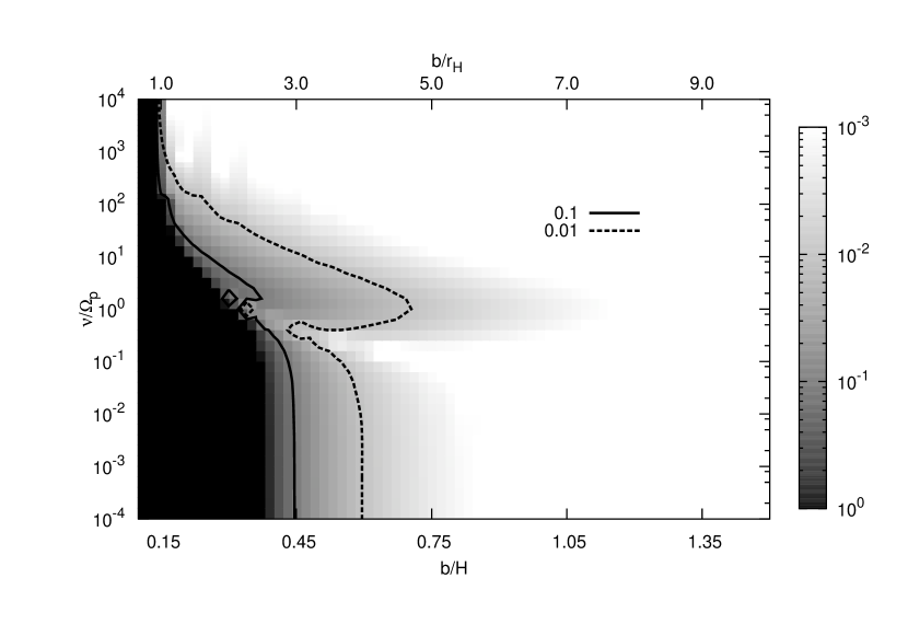
Figure 11: Deflection of the particle’s semi-major axis after the first encounter with the planet. The amount of deflection is quantified by equation (87). Horizontal axis denotes the particle’s initial semi-major axis and vertical axis denotes the particle’s drag, or equivalently, size. Initial semi-major axes are shown in terms of scale height (bottom axis) and Hill’s radius (top axis). Gray scale shows the amount of deflection, and the contours of 10% (solid line) and 1% (dashed line) deflection are shown. Particles in black regions are trapped by the planet (that is, mutual distance between the particle and the planet becomes smaller than half of Hill’s radius) or in horseshoe orbit.

where we have assumed $L_{y}\sim r_{\rm p}$, $\eta\sim(H/r_{\rm p})^{2}$ and all the numerical coefficients are neglected. For low mass planets which does not form a gap in the gas disk, Hill’s radius is generally smaller than the scale height. Therefore, the motion of the particle is predominated by the effect of global pressure gradient. However, for large planets with mass of order Jupiter, the effect of the global pressure gradient is small compared to the gravitational interaction between the planet, and equation (70) indicates that if the profile of the gas disk is neglected, the particles may be attracted towards the planet. This seems to be consistent with what is found by Paardekooper (2007). He found that when axisymmetric gas disk profile is considered, plants with the mass of the order of Jupiter would accrete the particles with stopping time comparable to Kepler time, while accretion of such particles around planets with 0.1 times Jupiter mass would be inefficient (see figures 7 and 11 of Paardekooper 2007). When global pressure gradient of gas disk drives the particles to migrate towards the central star, a part of particles with $\nu\sim\Omega_{\rm p}$ may pass the orbit of the planet without accumulating onto it, since the particle migration rate is very fast and the perturbation of the orbital elements of the particles is not related to the planet location (Kary et al. 1993). If the third term of equation (70) dominates over the global pressure effect, on the other hand, particles will accumulate onto the planet since their orbital elements are strongly perturbed at the location of the planet.

If the disk model with flat pressure profile is considered, the behavior of the particle around the planet is complicated. Figure 3 shows the contour plot of equation (70) for the planet mass $GM_{\rm p}/Hc^{2}=10^{-2}$, flat pressure profile ($\eta=0$), and no mass accretion onto the central star ($\zeta=0$). For small particles ($\nu\to\infty$), there is no secular motion of particles since all the terms of equation (70) vanishes if $\zeta=0$. The motion of small particles is determined by the strength of accretion of the background flow. For large particles ($\nu\to 0$), on the other hand, the fourth term, which is the gravitational scattering by the planet, is dominant and the particles are always repeled away from the planet. For particles with intermediate size ($\nu\sim\Omega_{\rm p}$), all the terms must be considered. Particles located sufficiently far away from the planet are scattered away because of the contribution from the last term of equation (70), which is due to the axisymmetric mode of the perturbed flow structure caused by the planet gravity. Particles at the intermediate distance ($b/H\sim 1$), on the other hand, are attracted towards the planet because of the third term. If the particles are close to the planet, they are again scattered away because of the contribution from gravitational scattering.

The equilibrium distance between the third and fourth term is given by equation (26), and this becomes close to the planet with increasing $\nu$, and it eventually becomes smaller than the Hill’s radius, where we expect that the particle motion is largely dominated by the planet’s gravity and our treatment of distant encounter breaks down. Therefore, we conclude that the particles with intermediate but still smaller drag coefficient, on one hand, will accumulate around the planet, but not fully accrete onto the planet. On the other hand, particles with larger drag coefficient will accrete onto the planet since gravitational scattering is ineffective in this case. Equating the equilibrium distance given by equation (26) to Hill’s radius, the critical drag coefficient separating these two regimes is of order $10\Omega_{\rm p}$.

We note that since equation (70) is obtained under the assumption of distant encounter, it does not accurately describe the dynamics of particles located within the Hill’s sphere of the planet. In Section 3, we perform a numerical calculation of Hill’s equations and investigate the validity of assumptions in the derivation of equation (70). It needs to be checked whether particles will really accrete onto the planet when they approach towards the planet. For close encounter, the detailed structure of the gas around the planet must be considered. Inaba & Ikoma (2003) have shown that the capture cross section of particles by the planet may be enhanced when the atmospheric structure is considered.

3 Numerical Calculation in Local Coordinate

3.1 Numerical Methods

To investigate the accuracy of the description by equation (70) for the evolution of orbital element of a particle whose semi-major axis is close to the planet embedded in a gaseous disk, we perform a series of numerical calculations and compare the results with equation (70).

In our calculation, we solve Hill’s equations (3) and (4) using fifth-order Runge-Kutta method with variable time step. We are primarily interested in the effects of spiral density wave and the gravitational force by the planet centered at the coordinate system: we neglect the effect of the global pressure gradient and mass accretion, $\eta=\zeta=0$. The velocity field of the gas is therefore

$$\delta\mbox{\boldmath$v$}_{g}=\delta\mbox{\boldmath$v$}^{(1)}+\delta\mbox{\boldmath$v$}^{(2)},$$ (72)

where $\delta\mbox{\boldmath$v$}^{(1)}$ and $\delta\mbox{\boldmath$v$}^{(2)}$ are first and second order perturbations, respectively, described in section 2.6. We also note that for gravitational force exerted by the planet, we use

$$\nabla{\displaystyle\frac{GM_{\rm p}}{\sqrt{x^{2}+y^{2}}}}.$$ (73)

We do not use the time-averaged force given by equations (A8) and (A9).

The modification of gas velocity due to the gravitational force by the planet is obtained by second-order perturbation analysis. We numerically integrate equations (35)-(37) for the first order solution and (2.6)-(2.6) for the second order solutions. We make use of Fourier transform methods presented by Goodman and Rafikov (2001). This method is particularly useful in calculating the gravitational potential produced by the density fluctuation. We fix the spatial resolution (therefore, the maximum wave number in Fourier space) $(\Delta x/H,\Delta y/H)$ to be $(9.8\times 10^{-3},7.8\times 10^{-2})$, which is enough to resolve the effective Lindblad resonance (see e.g., Artymowicz 1993). We fix the box size in the $y$-direction such that $-80H<y<80H$ and impose a periodic boundary condition. For the $x$-direction, the resolution in Fourier space in $k_{x}$ direction is varied from $10^{4}$ to $10^{6}$ according to $k_{y}$ in order to resolve very fast oscillation at $k_{x}\gg k_{y}$. We also use the linear window function given by Goodman and Rafikov (2001). We set softening parameter $\epsilon$ to be $0.01H$.

The box size of our calculation in $y$-direction is $-80H<y<80H$, to be consistent with the calculation of the modification of the velocity field. In integrating Hill’s equations, we impose a periodic boundary condition in the $y$-direction and integrate the equations of motion until $t=5000\Omega_{\rm p}^{-1}$. By periodic boundary condition, we mean that when the particle has reached the boundary of the box in $y$-direction, $y=\pm 80H$, it is reintroduced into the other end of the box, $y=\mp 80H$, while the values of $x$, $v_{x}$, and $v_{y}$ are kept unchanged. In principle, Hill’s equations describe the motion of the particle only in the vicinity of the planet, and hence there is no reason that the phase of the epicyclic motion is conserved when it is reintroduced. However, we expect that if the box size is the same as $2\pi r_{\rm p}$, which is the circumference of the disk at the orbit of the planet, this periodic boundary treatment may simulate qualitative properties of the orbit in the global calculations. The condition

$$L_{y}=2\pi r_{\rm p}$$ (74)

is realized, in the parameter of our calculations, if we consider a disk with the aspect ratio $H/r_{\rm p}=2\pi/160\sim 0.04$.

Once we know the data of $(x,\dot{x},y,\dot{y})$, we can calculate the osculating elements $(b,h,k)$ by, using equations (9) and (10),

$$b=4x+{\displaystyle\frac{2}{\Omega_{\rm p}}}\dot{y},$$ (75)

$$h=-{\displaystyle\frac{1}{r_{\rm p}\Omega_{\rm p}}}\left[\dot{x}\sin(\Omega_{\rm p}t)+2\left(\dot{y}+{\displaystyle\frac{3}{2}}x\Omega_{\rm p}\cos(\Omega_{\rm p}t)\right)\right],$$ (76)

$$k={\displaystyle\frac{1}{r_{\rm p}\Omega_{\rm p}}}\left[\dot{x}\cos(\Omega_{\rm p}t)-2\left(\dot{y}+{\displaystyle\frac{3}{2}}x\Omega_{\rm p}\sin(\Omega_{\rm p}t)\right)\right].$$ (77)

In the following sections showing results of calculations, we refer to $(b,h,k)$ using these relations. These values are not averaged over the encounter, but are defined at any time of the orbit.

The initial condition of the calculation is that the particles are located at the edge of the box and moving in a circular motion. When a particle approaches to the planet and the mutual distance becomes smaller than half of the Hill’s radius of the planet, we stop the calculation since we are primarily interested in the distant encounter. Such particles should be trapped by the planet’s gravity and eventually accrete onto the planet. In order to obtain a smooth results in the runs with large drag coefficient, we make use of smoothing methods described in Appendix D in calculating the perturbed gas velocity at the location of the particle from the data obtained by hydrodynamic equations. We fix the background density to be $10^{-10}\mathrm{g/cm}^{3}$, which is an order of magnitude smaller than the Minimum Mass Solar Nebula (Hayashi et al. 1985). Toomre’s $Q$ parameter of the disk at $1\mathrm{AU}$ with is

$$Q^{-1}\sim{\displaystyle\frac{G\rho}{\Omega_{\rm p}^{2}}}\sim 10^{-4}$$ (78)

We assume the mass of the planet as $GM_{\rm p}/Hc^{2}=10^{-2}$ that corresponds to $0.2M_{\oplus}$ for $c=10^{5}\mathrm{cm/s}$ and $H=0.05\mathrm{AU}$. In the following sections, we show the results without the gravitational force by gas. We have checked that gas gravity does not affect the results in our parameter range. We also neglect the effect of global pressure gradient and steady mass accretion in our calculation, $\eta=\zeta=0$, in order to see the effect of spiral wave and planet’s gravity.

3.2 Results

3.2.1 Properties of Orbital Evolution

We first review the properties of orbital evolution of a particle with zero friction force, which is obtained by setting $\nu=0$. Figure 4 shows the evolution of $b$ for a particle initially located at $b=H$. The values of $b$ are obtained according to equations (75) when the particle is at the box boundary. Also indicated in Figure 4 is the variation of $b$ for $0<t<250\Omega^{-1}$. The values of $b$ varies rapidly when the particle encounters with the planet, when $y\sim 0$. We note that since the box size is $160H$, time taken for the particle to cross the box is $\sim 160/(3/2)\sim 100$ Kepler times.

It is indicated that the semi-major axis difference $b$ first increases but then shows an oscillation with the period $\sim 1200$ Kepler times. This oscillation is caused by the excitation of eccentricity by the perturbation due to the planet. If the particle comes into the box with finite eccentricity, the distance between the particle and the planet at the closest approach is different depending on the phase of the epicyclic motion, and the semi-major axis of the particle can increase or decrease. The period and amplitude of this oscillation depend on the location of the particle. If the phase of the epicyclic motion among successive encounters between the planet and the particle matches, the period of the oscillation becomes longer and the amplitude becomes larger. The condition for strong amplification is given by

$$\Omega_{\rm p}T=2\pi l,$$ (79)

where $l$ is an integer and $T$ is the time taken to cross the box in $y$-direction

$$T={\displaystyle\frac{L_{y}}{(3/2)b\Omega_{\rm p}}}.$$ (80)

Figure 5 compares the evolution of semi-major axis of the particle starting at $l=5$ position ($b=3.4H$) and at $b=3.8H$. It is clear that the particle at $l=5$ position experiences the long-term, strong oscillation of semi-major axis.

Equation (79) indicates that there is a resonance between the box crossing time and the epicyclic motion of the particle, and this appears as a result of our treatment of periodic boundary in Hill’s coordinate. Thus, in general, we should not consider this resonance to be physical if we arbitrary choose the box size in the y-direction. However, if we take the box size $L_{y}$ as the circumference of the disk, $2\pi r_{\rm p}$, the crossing time $T$ corresponds to the period of synodic encounter. Therefore, it may be possible to interpret this resonance as $j/(j+1)$ resonances in global problems. In section 4, we explore the correspondence between the Hill’s approximation and the full global problem.

We now consider the problem with gas drag. Figure 6 shows the evolution of $b$ for particles with various drag coefficients initially located at $b/H=1$ as a function of time. The values of $b$ when the particles reach at the edge of the box are plotted. Particles with drag coefficient larger than $\nu/\Omega_{\rm p}=10^{-2}$ shows a systematic change of semi-major axis while that with $\nu/\Omega_{\rm p}=10^{-4}$ shows a systematic change plus oscillation. In a simple restricted three-body problem, where drag coefficient $\nu$ equals zero, semi-major axis does not show a systematic change but only oscillation, as discussed in previous paragraphs (see also Figures 4 and 5). The gas drag causes a systematic change of Jacobi energy and thereby results in a systematic change of particle’s angular momentum. The timescale during which the oscillation of semi-major axis damps is given by $\sim\nu^{-1}$. Since the oscillation of the semi-major axis comes from the excitation of eccentricity during the synodic encounter, this oscillation does not appear when the eccentricity is damped during successive encounters. If the eccentricity is damped during successive encounters, the assumption of initially circular orbit in deriving equation (70) is valid for every encounter. Therefore, although we have computed only one encounter, it is possible to use equation (70) to predict the long-term evolution of the orbital semi-major axis especially for small bodies with large drag coefficient.

3.2.2 Comparison between Analytic and Numerical Calculations

We now show to what extent equation (70) describes the evolution of the orbit of a particle encountering with a planet embedded in a gaseous nebula. Since the particles show a systematic change of semi-major axis, we take the average radial velocity of the particle by calculating

$${\displaystyle\frac{b(t_{\rm fin})-b(t_{\rm ini})}{t_{\rm calc}}},$$ (81)

where $t_{\rm ini}=0$ is the initial time, $t_{\rm fin}$ is the last time when the particle reaches the box boundary before the calculation is stopped at $t=5000\Omega^{-1}$, and $t_{\rm calc}=t_{\rm fin}-t_{\rm ini}$. The precise value of $t_{\rm fin}$ is obtained by numerical calculation, and it varies with the value of $b$. Semi-major axis of the particle at each time is calculated by equation (75).

Figures 7-9 show the results of long-term evolution of semi-major axis of particles initially located at various position with $\nu/\Omega_{\rm p}=10^{-2}$, $1$, and $10^{2}$ respectively. Horizontal axes of Figures 7-9 are the initial semi-major axis of the particle, $b(t_{\rm ini})$, and the vertical axes show the average rate of change of semi-major axes obtained by equation (81). We also plot our analytic formula given by (70). It is clear that the analytic formula (70) describes the results of numerical calculations well, at least quantitatively, for all values of drag coefficient. Deviation from the analytic value for $\nu/\Omega_{\rm p}=1$ at $b/H\mathrel{\hbox{\hbox to0.0pt{\hbox{\lower 4.0pt\hbox{$\sim$}}\hss}\hbox{$>$}}}2$ comes from the deviation of the data of $\overline{\delta v_{y}^{(1)}}$ from the analytic value shown in Figure 2 while for small $b$, we expect that the numerical results deviate from the analytic calculation since eccentricity effect is not negligible. The match between numerical calculation and analytic formula is better for particles with large drag coefficient, since their eccentricities remain smaller. We think that the deviation from the analytic value for $\nu/\Omega_{\rm p}=10^{2}$ at $b/H\mathrel{\hbox{\hbox to0.0pt{\hbox{\lower 4.0pt\hbox{$\sim$}}\hss}\hbox{$>$}}}3$ is due to smoothing.

One significant difference between analytic results and numerical calculation is the spike-like structures that appear in the calculations with $\nu/\Omega_{\rm p}=10^{-2}$. This structure is due to the resonance effect given by equation (79). We show in Figure 7 the location of resonance with $l=4$, $5$, and $6$. It is clear that $\Delta b/T$ shows a spike at this location. We have not found such resonance structure for calculations with $\nu/\Omega_{\rm p}\mathrel{\hbox{\hbox to0.0pt{\hbox{\lower 4.0pt\hbox{$\sim$}}\hss}\hbox{$>$}}}1$. This is because eccentricity is sufficiently damped between successive encounters.

Another interesting result is the motion of the particle with $\Omega_{\rm p}\sim\nu$. Figure 10 shows the evolution of the semi-major axes of the particles with $\nu/\Omega_{\rm p}=1$. It is clear that the particles migrate towards the planet and stagnate at $b\sim 0.35H$. Since we set $\eta=\zeta=0$ in our calculation, the orbital change of the particle is caused by the third, fourth, and fifth terms of equation (70). The last term is negligible for small $b$ compared to the third term. Equation (70) indicates that these particles accumulate near the planet’s orbit where gravitational scattering represented by the fourth term of equation (70) balances with the attraction towards the planet represented by the third term, which is the result of combination of the planet’s gravity and the gas drag, as discussed in Section 2.3. The condition for the balance between these two effects is given by equation (26). For chosen parameters in numerical calculations, $r_{\rm H}=0.15H$ so the equilibrium distance is given by $\sim 0.3H$, which is close to the value obtained in numerical calculation $\sim 0.35H$. We consider that the small difference comes from the effect of eccentricity and close encounter. This effect seems analogous to “the shepherding effect”. We note that this effect appears when the first term of equation (70), $\Delta b$ by global pressure gradient, is small compared to the third term. This condition is expressed in terms of $\eta$:

$$|\eta|<{\displaystyle\frac{r_{\rm p}}{b}}{\displaystyle\frac{r_{\rm H}^{3}}{r_{\rm p}^{3}}}\sim{\displaystyle\frac{r_{\rm p}}{b}}{\displaystyle\frac{M_{\rm p}}{M_{\ast}}}.$$ (82)

If $\eta$ is of the order of square of disk aspect ratio, as in standard parameters, this condition is rewritten as

$${\displaystyle\frac{b}{r_{\rm H}}}\mathrel{\hbox{\hbox to0.0pt{\hbox{\lower 4.0pt\hbox{$\sim$}}\hss}\hbox{$<$}}}\left({\displaystyle\frac{M_{\rm p}}{M_{\ast}}}\right)^{2/3}\left({\displaystyle\frac{r_{\rm p}}{H}}\right)^{2}.$$ (83)

For $M_{\rm p}/M_{\ast}=10^{-6}$ and $H/r_{\rm p}=0.05$, this gives $b/r_{\rm H}\mathrel{\hbox{\hbox to0.0pt{\hbox{\lower 4.0pt\hbox{$\sim$}}\hss}\hbox{$<$}}}0.2$, which is too close to the planet and the assumption of distant encounter is violated. Kary et al. (1993) has shown that, in the presence of global pressure gradient, a particle with $\nu\sim\Omega_{\rm p}$ falls onto the central star so rapidly that it bypasses the planet without being trapped.

3.3 Limitation of Analytic Formula

Equation (70) is derived by assuming that the deflection angle of the particle by each encounter with the planet is small (distant encounter) and that the particle returns to a circular orbit before the next encounter.

First, the assumption of initially circular orbit breaks down if we consider the particle with small friction. The oscillation of semi-major axis observed in figure 6 for particles with $\nu=10^{-4}\Omega_{\rm p}$ indicates that the damping of eccentricity between successive encounters is insignificant for these particles and that the finite eccentricity effect should be taken into account. Quantitatively, the period of synodic encounter must be longer than the particle’s stopping time. Therefore, our treatment is limited in the cases with

$${\displaystyle\frac{2\pi r_{\rm p}}{(3/2)b\Omega_{\rm p}}}\mathrel{\hbox{\hbox to0.0pt{\hbox{\lower 4.0pt\hbox{$\sim$}}\hss}\hbox{$>$}}}{\displaystyle\frac{1}{\nu}},$$ (84)

where the left hand side is the synodic period and the right hand side is stopping time. Rearranging this condition, we have

$${\displaystyle\frac{b}{H}}\mathrel{\hbox{\hbox to0.0pt{\hbox{\lower 4.0pt\hbox{$\sim$}}\hss}\hbox{$<$}}}{\displaystyle\frac{4\pi}{3}}{\displaystyle\frac{r_{\rm p}}{H}}{\displaystyle\frac{\nu}{\Omega_{\rm p}}}.$$ (85)

Adopting standard parameters, we have

$${\displaystyle\frac{b}{H}}\mathrel{\hbox{\hbox to0.0pt{\hbox{\lower 4.0pt\hbox{$\sim$}}\hss}\hbox{$<$}}}80\left({\displaystyle\frac{0.05}{H/r_{\rm p}}}\right)^{-1}\left({\displaystyle\frac{\nu/\Omega_{\rm p}}{1}}\right).$$ (86)

We now consider the assumption of distant encounter. If the particle’s semi-major axis is too close to the planet, the assumption of small deflection angle, or distant encounter, breaks down. In Figure 11, we plot the amount of deflection of the particle’s semi-major axis after the very first encounter with the planet. We quantify the amount of deflection by

$${\displaystyle\frac{|b(t_{1})-b(t_{2})|}{|b(t_{1})|}},$$ (87)

where $t_{1}=t_{\rm ini}=0$ is the initial time, and $t_{2}\sim L_{y}/(3/2)b\Omega_{\rm p}$ is the time when the particle reaches the box boundary after the first encounter. The precise value of $t_{2}$ is obtained by numerical calculations. Particles in black regions are trapped by the planet, that is, in our criterion, mutual distance between the planet and the particle becomes smaller than half of the Hill’s radius, or in horseshoe orbit. Note the similarity of the shape of the contour of 1% deflection with the contour shown in Figure 3.

In three-body problem with zero drag force, it is known that the assumption of small encounter is violated for particles with $b\mathrel{\hbox{\hbox to0.0pt{\hbox{\lower 4.0pt\hbox{$\sim$}}\hss}\hbox{$<$}}}2.5r_{\rm H}$ if we consider the very first encounter. Our calculation is consistent with this for particles with small drag, $\nu\ll\Omega_{\rm p}$. However, for particles with large drag, $\nu\gg\Omega_{\rm p}$, it can be seen that this condition is relaxed and it is indicated that the assumption of small deflection angle can be used even down to $b\sim r_{\rm H}$. Figure 12 shows the orbits of particles initially located at $b=2r_{\rm H}$. Orbits of particles with $\nu/\Omega_{\rm p}=10^{-4}$ and $10^{3}$ are shown. Particles with very large drag coefficient can remain in the orbit close to the initial semi-major axis since gas drag prevents it from falling onto the planet.

After multiple encounters, the condition of distant encounter is violated for particles with $b\mathrel{\hbox{\hbox to0.0pt{\hbox{\lower 4.0pt\hbox{$\sim$}}\hss}\hbox{$<$}}}2.5-2\sqrt{3}r_{\rm H}$ in three-body problem without gas drag. The contour of 1% deflection in Figure 11 passes close to $2\sqrt{3}r_{\rm H}$ in the limit of small drag. Therefore, we infer that this line gives the limitation of our analytic treatment assuming small deflection. This assumption is better for particles in wider range of semi-major axes for larger drag.

4 Comparison between Local and Global Calculation

So far we have performed analytic and numerical calculations of the orbits of particles using local coordinate systems. It remains to be checked how our local treatment simulates the real orbit in global coordinate.

We have performed a global calculation with the gas rotating at Keplerian rotation velocity where we have neglected the effect of the spiral pattern around the planet, global pressure gradient, and gas accretion towards the central star, $\eta=\zeta=0$. We solved the equations of motion in a frame rotating with the planet and integrate until the particle encounters with the planet for 100 times. We calculated the evolution of the semi-major axis of a particle at various initial semi-major axes and obtain $\Delta b/T$ over the calculation time. In the following, we show calculations in which the particle is located at the opposition point initially, but we have checked that the initial locations do not affect the results as long as we consider particles with $\nu/\Omega_{\rm p}\geq 10^{-2}$. Particles that reach the distance with the planet less than Hill’s radius are removed. We set disk aspect ratio $H/r_{\rm p}=0.04$, which gives $2\pi r_{\rm p}=L_{y}$, where $L_{y}=160H$ is the box size we have used in calculations with Hill’s equation. For planet mass, we assumed $M_{\rm p}/M_{\ast}=6\times 10^{-7}$, which corresponds to $GM_{\rm p}/Hc^{2}=10^{-2}$, the value we have adopted in calculations with Hill’s equations. In order to compare the results of global calculations with Hill’s equations, we also integrate Hill’s equations (3) and (4) by setting $\delta\mbox{\boldmath$v$}_{\rm g}=0$.

Figures 13-15 compare the results of $\Delta b/T$ obtained by global and local calculations. Horizontal axes of Figures 13-15 show the initial semi-major axes of the particle and the vertical axes show the average rate of change calculated by equation (81). In global calculations, $b(t_{\rm fin})$ is the semi-major axis difference between the particle and the particle calculated when the particle has reached the opposition point after 100 encounters.

For all parameters, global and local calculations show a reasonably good agreement. Relative difference between global and local runs is most significant for particles with ${\nu}/{\Omega_{\rm p}}=1$. We infer that this is because in the case of ${\nu}/{\Omega_{\rm p}}=1$, the radial motion of the particle is the fastest, and the effect of curvature is most effective. In runs with ${\nu}/{\Omega}_{\rm p}=10^{2}$ and ${\nu}/{\Omega}_{\rm p}=10^{-2}$, radial motion of the particle is smaller by one or two orders of magnitude than calculations with ${\nu}/{\Omega}_{\rm p}=1$.

In runs with $\nu/\Omega_{\rm p}=10^{-2}$, we observe a disagreement in resonance locations, since curvature effects are not taken into account. However, since the disagreement is less than 10%, it may be still possible to say, for example, that $l=4$ resonance in Hill’s coordinate mimics $4:5$ resonance in global coordinate. Note that the relative strength of the resonance matches well with global runs.

Global analysis of $j/(j+1)$ resonances including drag force is done by Greenberg (1978). It is shown that eccentricity and the angle between the longitude of conjunction and the longitude of pericenter of the particle converges to a fixed value with the timescale of $\nu^{-1}$, but depends on the particle’s semi-major axis. The value of eccentricity is maximum at the resonance. We have observed similar behavior in local calculations. It is actually possible to do analytic calculation similar to Greenberg (1978) in Hill’s system and derive orbital evolution including the effect of resonance. We do not show it here since it is necessary to do all the analyses presented in Section 2 again including the effect of finite box size. We simply note here that this resonance effect does not appear in our formulation presented in Section 2 since we have neglected the effect of finite length in the $y$-direction in deriving equation (70).

In runs with $\nu/\Omega_{\rm p}=1$, particles initially at $b\mathrel{\hbox{\hbox to0.0pt{\hbox{\lower 4.0pt\hbox{$\sim$}}\hss}\hbox{$<$}}}1.4H$ shows the decrease of the average rate of semi-major axis decay. This is because the particle is trapped in the orbit in the vicinity of the planet as a result of shepherding effect discussed for calculations with Hill’s equation in Section 3.2. Figure 16 shows the evolution of the semi-major axis of the particle. Osculating elements at the opposition points are plotted. Comparing with Figure 10, it is clear that the shepherding effect discussed in local calculations also exists in global runs. We note that the amplitude of oscillation after particles are trapped is larger in global runs than local calculations, and the location of the shepherding orbit is slightly closer to the planet than the local calculations. Note in passing that in equation (4.11) of Adachi et al. (1976), it is indicated that for $\eta=0$, damping of eccentricity causes a decrease in semi-major axis. However, Adachi et al. (1976) do not take into account the effects of the planet’s gravity. The shepherding presented here is entirely caused by the presence of the planet.

By comparing global calculations with local runs, it is indicated that as long as the orbits close enough to the planet are considered, local calculations reproduce the results of global calculations well even if curvature effect is neglected. However, the effect of constant box size in the $y$-direction causes the small difference between the global and local runs. This is indicated by the mismatch between the locations of the resonances. It is also indicated that the local calculations reproduce the results of global calculations most efficiently for small particles, such as $\nu/\Omega_{\rm p}\mathrel{\hbox{\hbox to0.0pt{\hbox{\lower 4.0pt\hbox{$\sim$}}\hss}\hbox{$<$}}}10^{-1}-10^{-2}$. Local approach that is used in Section 2 is valid when semi-major axis difference $b$ is much smaller than the scale of the semi-major axis of the planet:

$${\displaystyle\frac{b}{r_{\rm p}}}\ll 1,$$ (88)

which is equivalent to

$${\displaystyle\frac{b}{H}}\ll{\displaystyle\frac{r_{\rm p}}{H}}.$$ (89)

Note that in the usage of equation (70) there is another limitation of close encounter, which has already been addressed in Section 3.3.

5 Discussion: Dust Gap Opening

5.1 Order-of-Magnitude Estimate of Dust Gap Opening Criterion

Paardekooper and Mellema (2004, 2006) showed that dust gap may be opened up even if the planet mass is too small to open up a gap in a gas disk using numerical calculation. We reconsider this result from the analytical point of view in this section.

Since there is no long-term radial motion of fluid elements, it is essential in dust gap formation that gas and dust moves in a different velocity. Terms that are important in equation (70) are therefore those proportional to $\nu\Omega_{\rm p}/(\nu^{2}+\Omega_{\rm p}^{2})$ for small particles.

We first consider the disk without global pressure gradient. In this case, the motion of small dust particles are mainly dominated by the third term of equation (70) when they are as close to the planet as $b\mathrel{\hbox{\hbox to0.0pt{\hbox{\lower 4.0pt\hbox{$\sim$}}\hss}\hbox{$<$}}}2H$ and by the last term when $b$ is larger. The third term is the attraction of particles by the planet’s gravity and they migrate towards the planet. The last term on the other hand originates from the axisymmetric flow structure around the planet. This term causes dust particles migrate away from the planet. In either case, dust particles around the planet with $b\sim H$ forms a gap around the planet. Taking $b\sim H$, very rough order-of-magnitude estimate (neglecting numerical coefficients of order unity) gives the migration timescale of dust particles as

$$\tau_{\rm gap}\equiv b{\displaystyle\frac{T}{\Delta b}}\sim 10^{4-5}T_{\rm K}\left({\displaystyle\frac{10^{-5}}{M_{\rm p}/M_{\rm c}}}\right)\left({\displaystyle\frac{H/r_{\rm p}}{0.05}}\right)^{2}\left({\displaystyle\frac{(\nu^{2}+\Omega_{\rm p}^{2})/\nu\Omega_{\rm p}}{10^{2}}}\right)$$ (90)

where $T_{\rm K}$ denotes the Kepler timescale and $M_{\rm c}$ is the mass of the central star. This is the timescale of dust particles changing its orbit by the order of scale height and gives the timescale of the formation of dust gap with width of the order of the scale height.

If there is global pressure gradient, the first term of equation (70) may dominate over the terms considered above. Since global pressure gradient causes systematic inward or outward motion of particles, dust gap around the planet is not expected to form if this term dominates. The timescale of orbital change of dust particles by the order of scale height due to the first term of equation (70) is

$$\tau_{\eta}\sim 10^{3-4}T_{\rm K}\left({\displaystyle\frac{10^{-3}}{|\eta|}}\right)\left({\displaystyle\frac{H/r_{\rm p}}{0.05}}\right)\left({\displaystyle\frac{(\nu^{2}+\Omega_{\rm p}^{2})/\nu\Omega_{\rm p}}{10^{2}}}\right).$$ (91)

If the magnitude of $\eta$ is of order $(H/r_{\rm p})^{2}\sim 10^{-3}$, which is a standard value, dust gap may not appear around the planet since $\tau_{\eta}<\tau_{\rm gap}$. However if $\eta$ is as small as $10^{-5}$, dust gap formation may be possible. The value of $\eta$ depends on disk model and can take values of wide range. From theoretical point of view, small value of $\eta$ is preferable in order for meter-size particles to survive in a Minimum Mass Solar Nebula. One mechanism of decreasing $\eta$ around ice line is suggested by Kretke and Lin (2007).

Comparing the first and the third term of equation (70), we obtain the criterion of dust gap formation. Again, for $b\sim H$, and neglecting numerical coefficients of order unity, we have, for the gap formation criterion,

$$|\eta|{\displaystyle\frac{M_{\rm c}}{M_{\rm p}}}{\displaystyle\frac{H}{r_{\rm p}}}\mathrel{\hbox{\hbox to0.0pt{\hbox{\lower 4.0pt\hbox{$\sim$}}\hss}\hbox{$<$}}}1.$$ (92)

We note that this criterion does not depend on drag coefficient of the particles. However, the implicit assumption is that gravitational scattering, which is the fourth term of equation (70), is ineffective, which is proportianl to $\Omega_{\rm p}^{2}/(\nu^{2}+\Omega_{\rm p}^{2})$. Therefore, this condition applies to particles with $\nu\mathrel{\hbox{\hbox to0.0pt{\hbox{\lower 4.0pt\hbox{$\sim$}}\hss}\hbox{$>$}}}\Omega_{\rm p}$. Taking $\eta\sim(H/r_{\rm p})^{2}$ and $H/r_{\rm p}\sim 0.05$, this gives $M_{\rm p}/M_{\rm c}\mathrel{\hbox{\hbox to0.0pt{\hbox{\lower 4.0pt\hbox{$\sim$}}\hss}\hbox{$>$}}}10^{-4}$, which explains the condition obtained by Paardekooper and Mellema (2004, 2006).

Timescale constraint of dust gap formation may be obtained by comparing the above obtained timescale with the timescale of planet migration or gas dispersal timescale. Timescale of the type I planet migration of the radial distance comparable to the scale height is given by Tanaka et al. (2002) as

$$\tau_{\rm migI}\sim\Omega_{\rm p}{\displaystyle\frac{M_{\rm c}}{M_{\rm p}}}{\displaystyle\frac{M_{\rm c}}{\Sigma r_{\rm p}^{2}}}\left({\displaystyle\frac{H}{r_{\rm p}}}\right)^{3}.$$ (93)

Therefore, comparing this with $\tau_{\rm gap}$, we have

$${\displaystyle\frac{r_{\rm p}}{H}}{\displaystyle\frac{\Sigma r_{\rm p}^{2}}{M_{\rm c}}}{\displaystyle\frac{\nu^{2}+\Omega_{\rm p}^{2}}{\nu\Omega_{\rm p}}}\mathrel{\hbox{\hbox to0.0pt{\hbox{\lower 4.0pt\hbox{$\sim$}}\hss}\hbox{$<$}}}1.$$ (94)

Dust gap formation is efficient at late stage of planet formation when gas starts to dissipate and type I migration timescale becomes long. If $H/r_{\rm p}=0.05$ and $\Sigma r_{\rm p}^{2}/M_{\rm c}=10^{-3}$, this criterion gives $\nu/\Omega_{\rm p}\mathrel{\hbox{\hbox to0.0pt{\hbox{\lower 4.0pt\hbox{$\sim$}}\hss}\hbox{$<$}}}50$. If there is no type I migration, on the other hand, this constraint is relaxed and dust gap formation constraint is given by the timescale of disk gas dispersal, $\tau_{\rm gas}$. If $\tau_{\rm gas}$ is of the order of $10^{6}$ years, gap of particles with $\nu/\Omega_{\rm p}\mathrel{\hbox{\hbox to0.0pt{\hbox{\lower 4.0pt\hbox{$\sim$}}\hss}\hbox{$<$}}}10^{4}$ may be opened up.

5.2 Model of Radial Distribution of Dust Particles

In order to investigate the qualitative behavior of dust particles around the planet in long time, we model the motion of particles in the disk by one-dimensional advection equation

$${\displaystyle\frac{\partial N(t,b)}{\partial t}}+{\displaystyle\frac{\partial}{\partial b}}\left[v_{b}(b)N(t,b)\right]=0$$ (95)

where $v_{b}(b)$ is the radial velocity of the dust particles whose semi-major axis difference with the planet is $b$ and $N(t,b)$ is the appropriately normalized number of the particles with semi-major axis difference $b$ at time $t$. We use equation (70) for $v_{b}$ and solve (95) for $10^{6}\mathrm{yr}$ for particles with various drag coefficients. We have used second-order scheme with monotonicity condition (van Leer 1977). We fix $H$ and $c$ for simplicity in our computational domain and a planet with $GM_{\rm p}/Hc^{2}=10^{-1}$ is fixed at the origin. Planet mass corresponds to $2M_{\oplus}$ for $H=0.05\mathrm{AU}$ and $c=10^{5}\mathrm{cm/s}$. The computational domain is $r_{H}<b<10H$ and dust particles are homogeneously distributed initially: $N_{0}\equiv N(t=0,x)=1$ in this region. We have assumed that there is no dust particle out of this domain. For $T$ that appears in equation (70), we have assumed

$$T=2\pi/|\Omega_{K}(r_{p}+b)-\Omega_{K}(r_{p})|$$ (96)

where $\Omega_{K}$ is Keplerian angular velocity and $r_{p}$ is the location of the planet.

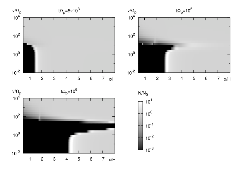
Figure 17: Time evolution of the distribution of dust particles around $2M_{\oplus}$ embedded in a solar nebula at $t\Omega_{\rm p}=5\times 10^{3}$ (top left), $t\Omega_{\rm p}=10^{5}$ (top right), and $t\Omega_{\rm p}=10^{6}$ (bottom left) with various $\nu$. The horizontal axis denotes the semi-major axis difference between the planet and the particle. Gray scale indicates the fraction of the remaining particles. The pressure gradient factor $\eta$ is set to be zero.

Figures 17 shows the snapshots of the distribution of dust particles of various drag coefficients at $t\Omega_{\rm p}=5\times 10^{3}$, $t\Omega_{\rm p}=10^{5}$, and $t\Omega_{\rm p}=10^{6}$ for $\eta=0$. The gap of particles with $\nu\sim 10\Omega_{\rm p}$ has been opened up after several $10^{5}$ Kepler time. The gap of particles $\nu\mathrel{\hbox{\hbox to0.0pt{\hbox{\lower 4.0pt\hbox{$\sim$}}\hss}\hbox{$<$}}}\Omega_{\rm p}$ may be the artefact of boundary condition, since the radial velocity of particles at the nearest edge of the planet is positive but we have assumed there is no dust particles outside the calculation domain. However, there is no boundary effect for small particles with large drag coefficient, since radial velocity of dust particle is negative at the inner edge and positive at the outer edge. We note that since it takes about $10^{5}$ years for dust gap formation for the planet with $2M_{\oplus}$, this effect is small if the gas pressure gradient is significantly large, $\eta>0$. However, for larger mass planets, planet perturbation on the dust motion is large and dust gap formation is possible even in the presence of pressure gradient, as seen in the order-of-magnitude estimate provided in the previous section.

Finally, we briefly discuss the observational implication of dust gap in the disk with zero pressure gradient. The width of the dust gap that forms around a low mass planet is several times the scale height. Therefore, it might be challenging to detect a low mass planet embedded in a gas disk at $1\mathrm{AU}$. However, if there is a planet at several tens of AU, the width of the gap can be of the order of several AU, which can be resolved in near future. The gap formation timescale in this case is of order $10^{5-6}$ years, which might be comparable to disk life time. Therefore, it may be possible to find a low mass planet by observing a dust gap in a gaseous nebula, even if the planet itself is too small to be observable.

6 Summary and Future Prospects

In this paper, we have investigated the motion of particles embedded in a gas disk in the presence of a small mass planet. This is the full analytic calculation of the particle motion including the gas disk and the planet considering the non-axisymmetric pattern of the gas around the planet produced by the gravitational interaction between the planet and the gas.

Our main result is equation (70) which describes the change of the particle semi-major axis, which has been in circular motion initially, after one distant encounter with the planet. In addition to well-known particle migration towards the central star due to the pressure gradient (the first term) and the gravitational scattering by the planet (fourth term), we have derived (1) the effect of steady mass accretion (the second term), (2) attraction of particles towards the planet due to the planet’s gravity (the third term), and (3) contribution of the structure of the gas disk produced by the planet’s gravity (the fifth term). We find that only the axisymmetric structure of the gas contributes to the semi-major axis evolution of particles and the spiral structure is ineffective in the absence of vorticity source.

All the terms considered, in the absence of the global pressure gradient and steady accretion flow towards the central star, we find that (see Figure 3) (1) particles with $\nu\mathrel{\hbox{\hbox to0.0pt{\hbox{\lower 4.0pt\hbox{$\sim$}}\hss}\hbox{$>$}}}\Omega_{\rm p}$ will migrate towards the planet if they are close to the planet because of the gravitational attraction by the planet, but they migrate away from the planet if they are far away, primarily due to the effect of the gas structure, (2) large particles with $\nu\ll\Omega_{\rm p}$ will be scattered away from the planet because of the gravitational scattering, and (3) there is a parameter range where particles are scattered away from the planet when they are close to the planet while attracted towards the planet if they are located at far away, thereby particles are accumulated at an equilibrium distance from the planet (i.e., shepherding by gas drag and gravitational scattering). This shepherding mechanism acts for particles in both interior and exterior orbits as long as the radial pressure gradient of the gas is negligible.

We have checked the validity of our formula by solving three-body problem with and without Hill’s approximations. Our main assumptions in deriving equation (70) are (1) initially circular orbit, (2) distant encounter, and (3) local approximation. Validity of the first assumption is justified when the eccentricity of the particle is damped within the time taken for each synodic encounter that is given by equation (86). The valid region for the second assumption is shown by the contour of small deflection in Figure 11. The condition for the third assumption is simply given by equation (89). Hill’s approximation is good as long as we consider the orbits in the vicinity of the planet. In short, our formula is especially useful in predicting the motions of dust particles with stopping time $t_{e}\Omega_{\rm p}\mathrel{\hbox{\hbox to0.0pt{\hbox{\lower 4.0pt\hbox{$\sim$}}\hss}\hbox{$<$}}}10^{2}$. For particles with smaller drag, our treatment predicts only quantitative behavior of non-resonant orbital evolution of particles whose semi-major axis is close to that of the planet. We also note that since we have made use of linear calculation for the flow, our treatment is restricted to low mass planets with the mass up to the orders of several tens of Earth mass.

Using equation (70), we have discussed the criterion for dust gap formation. The condition depends on the value of global pressure gradient, mass of the planet, and disk scale height. It is possible to derive the condition suggested by Paardekooper and Mellema (2004, 2006), and we have derived more general criteria. We have calculated the qualitative long-term behavior of dust particles around a planet with $2M_{\oplus}$. It is indicated that the gap of small dust particles with width of the order of several scale height may be opened up after several $10^{5}$ Kepler time. This long timescale has not been reached by full numerical simulations yet.

We have simplified the description of the drag force by assuming the force proportional to relative velocity with the gas. For large particles, however, the drag force is proportional to the square of the relative velocity, which is not treated in our calculation. We have also made a simplification by considering two-dimensional problem. In considering the vertical motion of particles, it is necessary to do three-dimensional calculations. The effects of magnetic field, self gravity, and turbulence of the disk will be the subjects in this line of analytical study. It is also of interest to extend our formulation to include the finite box size and investigate how the resonance effect is described in Hill’s system.

Appendix A Derivation of Equation (22)

In this section, we briefly show the derivation of (22). The method is the same as that of Goldreich and Tremaine (1980), Hénon and Petit (1986), or Hasegawa & Nakazawa (1990).

We consider the restricted three-body problem. In other words, we consider the problem with $\nu=0$. In this case, Jacobi energy $E_{J}$ conserves throughout the particle orbit. Jacobi energy is given by

$$E_{J}={\displaystyle\frac{1}{2}}r_{\rm p}^{2}\Omega_{\rm p}^{2}(h^{2}+k^{2})-{\displaystyle\frac{3}{8}}\Omega_{\rm p}^{2}b^{2}+\psi_{\rm p},$$ (A1)

where $\psi_{\rm p}$ is the gravitational potential of the planet. Therefore, orbital elements before and after the encounter with the planet are related by

$$-{\displaystyle\frac{3}{8}}\Omega_{\rm p}^{2}b^{2}={\displaystyle\frac{1}{2}}r_{\rm p}^{2}\Omega_{\rm p}^{2}(h(\infty)^{2}+k(\infty)^{2})-{\displaystyle\frac{3}{8}}\Omega_{\rm p}^{2}(b+\Delta b)^{2}.$$ (A2)

Assuming $\Delta b\ll b$, we obtain

$$\Delta b\sim{\displaystyle\frac{2r_{\rm p}^{2}}{3b}}\left(h(\infty)^{2}+k(\infty)^{2}\right).$$ (A3)

On the other hand, from equation (11), $\Delta b$ is given by

$$\Delta b={\displaystyle\frac{2}{\Omega_{\rm p}}}\int_{-\infty}^{\infty}F_{y}(t)dt.$$ (A4)

Therefore, we obtain

$$\int_{-\infty}^{\infty}F_{y}(t)dt={\displaystyle\frac{r_{\rm p}^{2}\Omega_{\rm p}}{3b}}(h(\infty)^{2}+k(\infty)^{2}).$$ (A5)

From equation (14) and (15), the elements $h$ and $k$ after the encounter are given by

$$h(\infty)=-{\displaystyle\frac{1}{r_{\rm p}\Omega_{\rm p}}}\int_{-\infty}^{\infty}du\left\{F_{x}(u)\sin[\Omega_{\rm p}u]+2F_{y}(u)\cos[\Omega_{\rm p}u]\right\}$$ (A6)

$$k(\infty)={\displaystyle\frac{1}{r_{\rm p}\Omega_{\rm p}}}\int_{-\infty}^{\infty}du\left\{F_{x}(u)\cos[\Omega_{\rm p}u]-2F_{y}(u)\sin[\Omega_{\rm p}u]\right\}.$$ (A7)

Approximating the trajectory of the particle by circular orbit, we have

$$F_{x}(t)\sim-\mathrm{sgn}(b){\displaystyle\frac{GM_{\rm p}}{b^{2}}}{\displaystyle\frac{1}{\left(1+(9/4)(\Omega_{\rm p}t)^{2}\right)^{3/2}}}$$ (A8)

$$F_{y}(t)\sim\mathrm{sgn}(b){\displaystyle\frac{GM_{\rm p}}{b^{2}}}{\displaystyle\frac{(3/2)\Omega_{\rm p}t}{\left(1+(9/4)(\Omega_{\rm p}t)^{2}\right)^{3/2}}}.$$ (A9)

Integrating (A6) and (A7), we have

$$h(\infty)=0$$ (A10)

$$k(\infty)=-\mathrm{sgn}(b){\displaystyle\frac{8}{9}}{\displaystyle\frac{1}{r_{\rm p}\Omega_{\rm p}^{2}}}{\displaystyle\frac{GM_{\rm p}}{b^{2}}}\left[K_{1}\left({\displaystyle\frac{2}{3}}\right)+2K_{0}\left({\displaystyle\frac{2}{3}}\right)\right].$$ (A11)

Substituting these results into equation (A5), we finally obtain

$$\int_{-\infty}^{\infty}F_{y}(t)dt={\displaystyle\frac{64}{243}}{\displaystyle\frac{G^{2}M_{\rm p}^{2}}{b^{5}\Omega_{\rm p}^{3}}}\left[K_{1}\left({\displaystyle\frac{2}{3}}\right)+2K_{0}\left({\displaystyle\frac{2}{3}}\right)\right]^{2}$$ (A12)

We note that direct substitution of equation (A9) into equation (A4) results in zero, indicating that higher order of the expansion is essential.

Appendix B Proof of Equation (66)

In this section, we show that the right hand side of equation (65) vanishes up to second order perturbation and prove equation (66). The equation we prove is

$$-{\displaystyle\frac{2}{\Omega_{\rm p}}}\displaystyle{\int_{0}^{T}}dt\delta v_{x}^{(1)}{\displaystyle\frac{\partial}{\partial x}}\delta v_{y}^{(1)}+\displaystyle{\int_{0}^{T}}dt_{1}{\displaystyle\frac{\partial\delta v_{x}^{(1)}}{\partial x}}(x_{c},y_{c}(t_{1}))\displaystyle{\int_{0}^{t_{1}}}dt_{2}\delta v_{x}^{(1)}(x_{c},y_{c}(t_{2}))$$

$$+\displaystyle{\int_{0}^{T}}dt_{1}{\displaystyle\frac{\partial\delta v_{x}^{(1)}}{\partial y}}(x_{c},y_{c}(t_{1}))\displaystyle{\int_{0}^{t_{1}}}dt_{2}\delta v_{y}^{(1)}(x_{c},y_{c}(t_{2}))=0$$ (B1)

We Fourier transform the perturbation in the $y$-direction,

$$\delta f(x,y)=\overline{\delta f}+\sum_{k_{y}\neq 0}\tilde{\delta f}_{k_{y}}(x)e^{ik_{y}y}$$ (B2)

where $\delta f$ denotes any perturbation quantity, $\overline{\delta f}$ is the average over $y$, and $\tilde{f}_{k_{y}}$ is the Fourier component of non-axisymmetric modes. Since physical quantities are real, $\tilde{\delta f}_{k_{y}}=\tilde{\delta f}_{-k_{y}}^{\ast}$. In this section, we drop superscript $(1)$ since all the perturbed values refer to first order values.

Since we integrate over the circular orbit, integration with respect to $t$ is converted to that with respect to $y$ by

$$y=-{\displaystyle\frac{3}{2}}x_{c}\Omega_{\rm p}t.$$ (B3)

It is possible to show that the right hand side of equation (B1) is equal to

$$-{\displaystyle\frac{8L_{y}}{3\Omega_{\rm p}x_{c}}}\sum_{k_{y}>0}\mathrm{Re}\left[\tilde{d\delta v_{x}}_{k_{y}}{\displaystyle\frac{\tilde{\delta v_{y}}_{k_{y}}^{\ast}}{dx}}\right]-{\displaystyle\frac{8L_{y}}{9\Omega_{\rm p}^{2}x_{c}^{2}}}\sum_{k_{y}>0}{\displaystyle\frac{1}{k_{y}}}\mathrm{Im}\left[{\displaystyle\frac{d\tilde{\delta v_{x}}_{k_{y}}^{\ast}}{dx}}\tilde{\delta v_{x}}_{k_{y}}\right]$$

$$+{\displaystyle\frac{8L_{y}}{9\Omega_{\rm p}^{2}x_{c}^{2}}}\sum_{k_{y}>0}\left[\tilde{\delta v_{x}}_{k_{y}}^{\ast}\tilde{\delta v_{y}}_{k_{y}}\right]+{\displaystyle\frac{4L_{y}}{9\Omega_{\rm p}^{2}x_{c}^{2}}}\overline{\delta v_{y}}\delta v_{x}(x_{c},L_{y}/2).$$ (B4)

The last term is zero as long as the box size is large enough. Using equation of continuity

$$-{\displaystyle\frac{3}{2}}ik_{y}x\Omega_{\rm p}{\displaystyle\frac{\tilde{\delta\Sigma}_{k_{y}}}{\Sigma_{0}}}+{\displaystyle\frac{d}{dx}}\tilde{\delta v_{x}}_{k_{y}}+ik_{y}\tilde{\delta v_{y}}=0$$ (B5)

and conservation of vorticity

$${\displaystyle\frac{d}{dx}}\tilde{\delta v_{y}}_{k_{y}}-ik_{y}\tilde{\delta v_{x}}_{k_{y}}-{\displaystyle\frac{1}{2}}\Omega_{\rm p}{\displaystyle\frac{\tilde{\delta\Sigma}_{k_{y}}}{\Sigma_{0}}}=0,$$ (B6)

we can show that the first three terms cancel. Hence, equation (66) is proved.

Appendix C Mass Flux of Sound Wave Propagating in a Homogeneous, Static Medium

In this section, we demonstrate that the sound wave that propagates in a homogeneous, non-rotating medium carries mass flux, and therefore, show that the vanishing mass flux given by equation (67) is not a general conclusion but specific to the problem in consideration. We consider one-dimensional system which extends in $x>0$, and at $x=0$, there is a forcing that creates a sound wave, which is turned on at $t=0$. The full system of equations are the equation of continuity and Euler equation in one-dimensional system

$${\displaystyle\frac{\partial\rho}{\partial t}}+{\displaystyle\frac{\partial}{\partial x}}(\rho x)=0$$ (C1)

$${\displaystyle\frac{\partial v}{\partial t}}+v{\displaystyle\frac{\partial v}{\partial x}}=-{\displaystyle\frac{c^{2}}{\rho}}{\displaystyle\frac{\partial\rho}{\partial x}}+S\cos(\Omega t)\delta_{D}(x)\theta(t),$$ (C2)

where $\rho$ is density, $v$ is velocity, $c$ is sound speed, $S$ is the amplitude of the source, $\Omega$ is the frequency of the forcing, $\delta_{D}(x)$ is the Dirac’s delta function, and $\theta(t)$ is step function. We consider background state with constant density $\rho_{0}$ and vanishing velocity.

The first order fluctuation caused by the forcing is given by

$${\displaystyle\frac{\partial}{\partial t}}{\displaystyle\frac{\delta\rho^{(1)}}{\rho_{0}}}+{\displaystyle\frac{\partial}{\partial x}}\delta v^{(1)}=0$$ (C3)

$${\displaystyle\frac{\partial}{\partial t}}\delta v^{(1)}+c^{2}{\displaystyle\frac{\partial}{\partial x}}{\displaystyle\frac{\delta\rho}{\rho_{0}}}=S\cos(\Omega t)\delta(x)\theta(t)$$ (C4)

and the second order perturbation is caused by the first order perturbation as follows

$${\displaystyle\frac{\partial}{\partial t}}{\displaystyle\frac{\delta\rho^{(1)}}{\rho_{0}}}+{\displaystyle\frac{\partial}{\partial x}}\delta v^{(1)}=-{\displaystyle\frac{\partial}{\partial x}}\left[{\displaystyle\frac{\delta\rho^{(1)}}{\rho_{0}}}\delta v^{(1)}\right]$$ (C5)

$${\displaystyle\frac{\partial}{\partial t}}\delta v^{(1)}+c^{2}{\displaystyle\frac{\partial}{\partial x}}{\displaystyle\frac{\delta\rho}{\rho_{0}}}={\displaystyle\frac{1}{2}}{\displaystyle\frac{\partial}{\partial x}}\left[c^{2}\left({\displaystyle\frac{\delta\rho^{(1)}}{\rho_{0}}}\right)^{2}-\delta v^{(1)^{2}}\right].$$ (C6)

Mass flux $F_{M}=\rho v$ is given by, up to the second order,

$$F_{M}=\rho_{0}\delta v^{(1)}+\rho_{0}\delta v^{(2)}+\delta\rho^{(1)}\delta v^{(1)}$$ (C7)

Since the sound wave propagates to $x\to\infty$ and there is no reflection, the appropriate solution for the first order is given by

$${\displaystyle\frac{\delta\rho^{(1)}}{\rho_{0}}}={\displaystyle\frac{S}{c^{2}}}\cos(\Omega t-kx),$$ (C8)

$$\delta v^{(1)}={\displaystyle\frac{S}{c}}\cos(\Omega t-kx)$$ (C9)

where $k=\Omega/c$ and the boundary condition at $x=0$ is considered.

Equation for second order velocity fluctuation is given by

$$\left[-{\displaystyle\frac{1}{c^{2}}}{\displaystyle\frac{\partial^{2}}{\partial t^{2}}}+{\displaystyle\frac{\partial^{2}}{\partial x^{2}}}\right]\delta v^{(2)}=2{\displaystyle\frac{k^{2}S^{2}}{c^{3}}}\cos\left[2(\Omega t-kx)\right].$$ (C10)

Since all the perturbation must vanish at $t=0$, we obtain

$$\delta v^{(2)}=-{\displaystyle\frac{S^{2}}{2c^{3}}}\Omega t\sin\left[2(\Omega t-kx)\right].$$ (C11)

Therefore, mass flux is given by

$$F_{M}={\displaystyle\frac{\rho_{0}S^{2}}{2c^{3}}}+{\displaystyle\frac{\rho_{0}S}{c}}\cos\left[\Omega t-kx\right]+{\displaystyle\frac{\rho_{0}S^{2}}{2c^{3}}}\Omega t\sin\left[2(\Omega t-kx)\right]+{\displaystyle\frac{\rho_{0}S^{2}}{2c^{3}}}\cos\left[2(\Omega t-kx)\right].$$ (C12)

Therefore, there is a positive and finite mass flux $\rho_{0}S^{2}/2c^{3}$ remains even after spatial and temporal averages are taken. It is also possible to show that a fluid element move to $x>0$ on average by calculating path line.

Appendix D Interpolation Methods

In the numerical calculation of large drag coefficient, stopping time of the particle $\nu^{-1}$ is very small that the particle remains in the same grid cell of the hydrodynamic calculation for several time steps. In this situation, it is necessary to have a smooth data of gas velocity even in sub-grid scale in order to obtain a smooth results. In this section, we describe how this can be realized.

Our method of interpolation is to consider the value of one grid cell as a representative value of physical data around the grid cell with a certain width, and add the contribution from nearby grid cells to find the value of physical quantities at a location of interest. Let $f(x)$ be the value of a physical quantity of interest and the data of $f(x)$ is given at discrete set of grid cells at $x=x_{i}$. We denote the data of $f(x)$ at $x=x_{i}$ by $f_{i}=f(x_{i})$ and $\Delta$ by grid size $\Delta=x_{i+1}-x_{i}$. Let the grid cell which is closest to the location of interest $x$ be $x_{i0}$. Our method of interpolation approximate the value of $f$ at $x$ by

$$f(x)\sim{\displaystyle\frac{\sum_{i=i0-I}^{i=i0+I}f_{i}\exp[-(x_{i}/\eta\Delta)^{2}]}{\sum_{i=i0-I}^{i=i0+I}\exp[-(x_{i}/\eta\Delta)^{2}]}}$$ (D1)

where $I$ is an integer and $\eta$ is a numerical factor. If $\eta$ is large, we have a more smoothed but more damped value. We find $I=20$ and $\eta=4$ gives a reasonably smooth results.

Figure 1: An example of the relationship between the dust size and the drag coefficient $\nu$ used in our numerical calculations, given by equation (8). Reciprocal of stopping time, $\nu=t_{e}^{-1}$ is shown as a function of dust size in centimeters for gas densities with $\rho=10^{-8}\mathrm{g/cm}^{3}$, $\rho=10^{-10}\mathrm{g/cm}^{3}$, and $\rho=10^{-12}\mathrm{g/cm}^{3}$.

Figure 2: Comparison between the azimuthally averaged profile of $L_{y}\delta v_{y}/c$ obtained by the numerical calculation (solid line) and analytic expression (53) (dotted line). The results of the numerical calculation is normalized by $GM_{\rm p}/Hc^{2}$.

Figure 3: Contour plot of $\Delta b/T$ given by equation (70) normalized by $H\Omega_{\rm p}$ for a planet with $GM_{\rm p}/Hc^{2}=10^{-2}$. The horizontal axis shows the distance from the planet and the vertical axis shows the drag coefficient of the particle. Global pressure gradient and steady mass accretion is neglected ($\eta=\zeta=0$). We note that our analytic approach is limited by assumptions of local approximation, initially circular orbit of the particle, and distant encounter. This figure has only qualitative meanings for particles with $\nu/\Omega_{\rm p}\mathrel{\hbox{\hbox to0.0pt{\hbox{\lower 4.0pt\hbox{$\sim$}}\hss}\hbox{$<$}}}10^{-2}$, with initial semi-major axis difference $b\mathrel{\hbox{\hbox to0.0pt{\hbox{\lower 4.0pt\hbox{$\sim$}}\hss}\hbox{$<$}}}3r_{\rm H}$ for $\nu/\Omega_{\rm p}\mathrel{\hbox{\hbox to0.0pt{\hbox{\lower 4.0pt\hbox{$\sim$}}\hss}\hbox{$<$}}}1-10$, or with $b\mathrel{\hbox{\hbox to0.0pt{\hbox{\lower 4.0pt\hbox{$\sim$}}\hss}\hbox{$<$}}}r_{\rm H}$ for $\nu/\Omega_{\rm p}\mathrel{\hbox{\hbox to0.0pt{\hbox{\lower 4.0pt\hbox{$\sim$}}\hss}\hbox{$>$}}}10$. Detailed discussions in the limitation of analytic calculations are given in Sections 3.3 and 4, and are summarized in Section 6.

Figure 4: Evolution of $b$ for a particle with zero drag coefficient initially located at $b=H$. Symbols show the values of $b$ obtained at the box boundary. The value of $b$ during the encounter is also indicated by dashed line upto $t=250\Omega_{\rm p}^{-1}$.

Figure 5: Evolution of $b$ for a particle with zero drag coefficient initially located at $b_{\rm ini}=3.4H$ (plus) that corresponds to $l=5$ case in equation (79) and $b_{\rm ini}=3.8H$ (cross) that does not satisfy equation (79). Vertical axis indicates the value of $(b(t)-b_{\rm ini})/H$. The value of $b(t)$ is obtained when the particle reaches the box boundary. Note that vertical axis of this figure is in logarithmic scale and the values smaller than $10^{-9}$ are not plotted. Horizontal axis shows time.

Figure 6: Evolution of $b$ for particles initially located at $x=H$ with different drag coefficient. Planet mass corresponds to $GM_{\rm p}/Hc^{2}=10^{-2}$. Particles with small drag coefficients shows oscillation, while particles with large drag coefficient shows a systematic decrease or increase of semi-major axis.

Figure 7: Comparison between the local numerical calculation (solid line) and analytical formula (dashed line) of $\Delta b/T$ for particles with $\nu/\Omega_{\rm p}=10^{-2}$. The value of $\Delta b/T$ is the average of a number of encounters and calculated using equation (81). The gravitational force by the planet and the spiral pattern of the gas around the planet are both considered.

Figure 8: Same as Figure 7 but for particles with $\nu/\Omega_{\rm p}=1$.

Figure 9: Same as Figure 7 but for particles with $\nu/\Omega_{\rm p}=10^{2}$.

Figure 10: Long-term evolution of the semi-major axis of the particles with $\nu=\Omega_{\rm p}$. The mass of the planet corresponds to $GM_{\rm p}/Hc^{2}=10^{-2}$. The calculations are done for the disk model with zero pressure gradient and zero accretion flow, $\eta=\zeta=0$.

Figure 12: Examples of the orbit of the particle when they encounter with the planet. Particles with $\nu/\Omega_{\rm p}=10^{-4}$ (solid line) and $\nu/\Omega_{\rm p}=10^{3}$ (dashed line) are shown. Both particles are initially located at $b=2r_{\rm H}$. Only the region $(1r_{\rm H}<x<2r_{\rm H},-50r_{\rm H}<y<50r_{\rm H})$ is shown. The particle with small drag is strongly perturbed by the planet and eventually captured within the Hill’s radius, while that with large drag can escape owing to the drag by the background gas.

Figure 13: Comparison between the global numerical calculation (solid line) and local calculation (dashed line) of $\Delta b/T$ for particles with $\nu/\Omega_{\rm p}=10^{-2}$. The average of the change of the semi-major axis of the particle after 100 encounters with the planet is shown. Horizontal axis shows the initial location of the particle normalized by disk scale height, $b/H=(r-r_{\rm p})/H$. We use disk aspect ratio $H/r_{\rm p}=0.04$ and the mass ratio between the planet and the central star is $M_{\rm p}/M_{\ast}=6\times 10^{-7}$. The disk aspect ratio is chosen in such a way that the value of $L_{y}$ we have adopted in the integration of Hill’s equation corresponds to $2\pi r_{\rm p}$, and the planet mass is chosen in such a way that $GM_{\rm p}/Hc^{2}=10^{-2}$, which is also the value we have used in local calculations. Keplerian rotation of the gas is assumed so $\eta=\zeta=0$ and there is no modification of the gas structure by the planet’s gravity. Note that global calculations and local calculations are in good agreement except for the location of the resonances. The position of $4:5$, $5:6$, and $6:7$ resonances are indicated by arrows.

Figure 14: Same as Figure 13 but for particles with $\nu/\Omega_{\rm p}=1$. Particles initially located at $b/H<1.4$ has been trapped in the vicinity of the resonance so the average rate of orbital change over 100 encounters is small. See also Figures 10 and 16 for the time evolution of semi-major axis difference $b$ for particles with $b/H\mathrel{\hbox{\hbox to0.0pt{\hbox{\lower 4.0pt\hbox{$\sim$}}\hss}\hbox{$<$}}}1.4$.

Figure 15: Same as Figure 13 but for particles with $\nu/\Omega_{\rm p}=10^{2}$.

Figure 16: Evolution of semi-major axis of particles with $\nu/\Omega_{\rm p}=1$ in global run with $\eta=\zeta=0$ and the gas is assumed to rotate at Kepler velocity. Osculating elements of the particle at the opposition point is plotted. Particles in both interior and exterior orbits migrate towards the planet and trapped in the orbit of $\sim 0.3H$. This figure corresponds to Figure 10 that shows the results of local calculations.

References

- Adachi et al. (1976) Adachi, I, Hayashi, C & Nakazawa, K. 1976, Prog. Theo. Phys., 56, 1756
- Artymowicz (1993) Artymowicz, P. 1993, ApJ, 419, 155
- Fouchet et al. (2008) Fouchet, L., Maddison, S. T., Gonzalez, J.-F., & Murray, J.R., 2007, A&A 474, 1037
- Goldreich and Tremaine (1979) Goldreich, P. & Tremaine, S. 1979, ApJ, 233, 857
- Goldreich and Tremaine (1980) Goldreich, P. & Tremaine, S. 1980, ApJ, 241, 425
- Goodman and Rafikov (2001) Goodman, J & Rafikov, R. R. 2001, ApJ, 552, 793
- Greenberg (1978) Greenberg, R. 1978, Icarus, 33, 62
- Haisch et al. (2001) Haisch, K., E., Lada, E., A., & Lada, C. J. 2001, ApJ, 553, L153
- Hasegawa and Nalazawa (1990) Hasegawa, M. & Nakazawa, K. 1990, A&A, 227, 619
- Hayashi et al. (1985) Hayashi, C., Nakazawa, K., & Nakagawa, Y. 1985, in Protostars and Planets II, ed. Black & Matthews (Tucson: Univ. Arizona Press)
- Hénon and Petit (1986) Hénon, M. & Petit, J-M. 1986, Celes. Mech, 38, 67
- Inaba and Ikoma (2003) Inaba, S. & Ikoma, M. 2003, A&A, 410, 711
- Kary et al. (1993) Kary, D. M., Lissauer, J. J., & Greenzweig, Y. 1993, Icarus, 106, 288
- Kretke and Lin (2007) Kretke, A. K. & Lin, D. N. C. 2007, ApJ, 664, L55
- Landau and Lifshitz (1959) Landau, L. D. & Lifshitz E. M., 1959, Fluid Mechanics, Course of Theoretical Physics (Oxford: Pergamon Press)
- Lyra et al. (2008) Lyra, W, Johansen, A., Klahr, H., & Piskunov, N. preprint (arXiv:0810.3192)
- van Leer (1977) van Leer, B. 1977, J. Comp. Phys., 23, 276
- Mizuno et al. (1978) Mizuno, H., Nakazawa, K., & Hayashi, C. 1978, Prog. Theo. Phys, 60, 699
- Narayan et al. (1987) Narayan, R., Goldreich, P., & Goodman, J. 1987, MNRAS, 228, 1
- Paardekooper (2007) Paardekooper, S.-J. 2007, A&A, 462, 355