Density gradients for the exchange energy of electrons in two dimensions

Abstract

We derive a generalized gradient approximation to the exchange energy to be used in density functional theory calculations of two-dimensional systems. This class of approximations has a long and successful history, but it has not yet been fully investigated for electrons in two dimensions. We follow the approach originally proposed by Becke for three-dimensional systems [Int. J. Quantum Chem. 23, 1915 (1983), J. Chem. Phys. 85, 7184 (1986)]. The resulting functional depends on two parameters that are adjusted to a test set of parabolically confined quantum dots. Our exchange functional is then tested on a variety of systems with promising results, reducing the error in the exchange energy by a factor of 4 with respect to the simple local density approximation.

I Introduction

Present nanoscale electronic devices contain a large variety of low-dimensional systems in which the many-body problems of interacting electrons need to be addressed. These systems include, e.g., modulated semiconductor layers and surfaces, quantum Hall systems, spintronic devices, and quantum dots qd . In order to describe the electronic properties of these systems, a practical and accurate way of computing the energy components is required. Since the advent of density-functional theory dft1 ; dft2 ; dft3 (DFT) much effort went into the development of approximate functionals for the exchange and correlation energies. Most of this work focused on three-dimensional (3D) systems, where considerable advances beyond the commonly used local density approximation (LDA) were achieved by generalized gradient approximations (GGAs), orbital functionals, and hybrid functionals functionals . However, previous studies have shown that most functionals developed for 3D systems break down when applied to two-dimensional (2D) systems kim ; pollack .

Within the DFT approach, 2D systems are most commonly treated using the 2D-LDA exchange [see Eq. (13) in Ref. rajagopal, ], which is then combined with the 2D-LDA correlation parametrized first by Tanatar and Ceperley tanatar and later, for the complete range of collinear spin polarization, by Attaccalite and co-workers attaccalite . Despite the relatively good performance of LDA with respect to, e.g., quantum Monte Carlo calculations henri , there is a clear lack of accurate 2D density functionals.

The exact-exchange functional employed within the optimized effective potential method, which automatically conforms to various dimensionalities, seems an appealing alternative to the LDA, and it has recently been applied to quantum dots nicole . In that method, however, the development of approximations for the correlation energies compatible with exact-exchange energies remains a complicated problem.

The derivation of local and semi-local approximations for the exchange-correlation energy in 2D can be carried out following the general lines already employed for the 3D case. In this way one can take advantage of the almost 40 years of experience in that field. Only very recently, such efforts have been done in 2D by developing exchange functionals specially tailored for finite 2D systems. pittalis ; ring ; ususus ; correlation In this work we take the most natural step beyond the LDA by including the density gradients in the functional. To this end, there are several possible approaches, e.g., the gradient expansion of the exchange hole perdew1 , semiclassical expansions from the Dirac or Bloch density matrix, dft1 and the GGAs of Perdew perdew2 and Becke. becke2 ; becke3 ; becke88 Here we follow the approach introduced by Becke for 3D systems in Refs.  becke2, and  becke3, , and derive and apply a GGA for the exchange energy of 2D electronic systems. Tests for a diverse set of 2D quantum dots show excellent performance of the derived approximation when compared with exact-exchange results.

II Derivation of the approximations

Within the Kohn-Sham approach to spin-DFT BarthHedin:72 , the ground state energies and spin densities $n_{\sigma}({\bf r})$ of a system of $N=N_{\uparrow}+N_{\downarrow}$ interacting electrons are determined. The total energy, which is minimized to obtain the ground-state energy, is written as a functional of the spin densities (in Hartree atomic units)

$$E[n_{\sigma}]=T_{\text{s}}[n_{\sigma}]+E_{\rm H}[n]+E_{\text{xc}}[n_{\sigma}]\\ +\sum_{\sigma=\uparrow,\downarrow}\int\!\!{\rm d}^{2}r\>v_{\sigma}({\bf r})n_{\sigma}({\bf r}),$$ (1)

where $T_{\text{s}}[n_{\sigma}]$ is the Kohn-Sham kinetic energy functional, $v_{\sigma}({\bf r})$ is the external (local) spin-dependent scalar potential acting upon the interacting system, $E_{\rm H}[n]$ is the classical electrostatic or Hartree energy of the total charge density $n({\bf r})=n_{\uparrow}({\bf r})+n_{\downarrow}({\bf r})$, and $E_{\text{xc}}[n_{\sigma}]$ is the exchange-correlation energy functional. The latter can be further decomposed into the exchange and correlation parts as $E_{\text{xc}}=E_{\text{x}}+E_{\text{c}}$.

In this work we focus in the exchange-energy functional, that can be expressed as

$$E_{\text{x}}[n_{\sigma}]=-\frac{1}{2}\sum_{\sigma=\uparrow,\downarrow}\int\!\!{\rm d}^{2}r_{1}\>\!\!\int\!\!{\rm d}^{2}r_{2}\>\frac{n_{\sigma}({\bf r}_{1})}{|{\bf r}_{1}-{\bf r}_{2}|}h_{\text{x},\sigma}({\bf r}_{1},{\bf r}_{2}),$$ (2)

where, within the restriction that the noninteracting ground state is nondegenerate and hence takes the form of a single Slater determinant, the exchange-hole (or Fermi-hole) function is given by

$$h_{\text{x},\sigma}({\bf r}_{1},{\bf r}_{2})=\frac{|\sum_{k=1}^{N_{\sigma}}\varphi^{*}_{k,\sigma}({\bf r}_{1})\varphi_{k,\sigma}({\bf r}_{2})|^{2}}{n_{\sigma}({\bf r}_{1})}.$$ (3)

The sum in the numerator is the one-body spin-density matrix of the Slater determinant constructed from the Kohn-Sham orbitals, $\varphi_{k,\sigma}$. Moreover, integrating this function over ${\bf r}_{2}$ yields

$$\int\!\!{\rm d}^{2}r_{2}\>h_{\text{x},\sigma}({\bf r}_{1},{\bf r}_{2})=1.$$ (4)

This exact property reflects the fact that around an electron with spin $\sigma$ at ${\bf r}_{1}$, other electrons of the same spin are less likely to be found. This a consequence of the Pauli principle. From Eq. (2) it is clear that to evaluate the exchange energy in 2D, we just need to know the cylindrical average w.r.t. ${\bf s}={\bf r}_{2}-{\bf r}_{1}$ of the exchange-hole around ${\bf r}_{1}$,

$$\bar{h}_{\text{x},\sigma}({\bf r}_{1},s)=\frac{1}{2\pi}\int_{0}^{2\pi}\!\!{\rm d}\phi_{s}\>h_{\text{x},\sigma}({\bf r}_{1},{\bf r}_{1}+{\bf s}),$$ (5)

from which

$$E_{\text{x}}[n_{\sigma}]=-\pi\sum_{\sigma=\uparrow,\downarrow}\int\!\!{\rm d}^{2}r\>n_{\sigma}({\bf r})\int\!\!{\rm d}s\>\bar{h}_{\text{x},\sigma}({\bf r},s),$$ (6)

where we have renamed ${\bf r}_{1}$ as ${\bf r}$. Expressing the exchange hole by its Taylor expansion, and considering its cylindrical average, one arrives at the following expression,

$$\bar{h}_{\text{x},\sigma}({\bf r},s)=n_{\sigma}({\bf r})+C^{\sigma}_{\text{x}}({\bf r})s^{2}+\ldots,$$ (7)

where $C^{\sigma}_{\text{x}}$ is the so-called local curvature of the exchange hole around the given reference point ${\bf r}$. This function can be expressed as becke2 ; Dobson:93 ; pittalis ; esa

$$C^{\sigma}_{\text{x}}({\bf r})=\frac{1}{4}\left[\nabla^{2}n_{\sigma}({\bf r})-2\tau_{\sigma}({\bf r})+\frac{1}{2}\frac{\left|\nabla n_{\sigma}({\bf r})\right|^{2}}{n_{\sigma}}+2\frac{{\bf j}^{2}_{p,\sigma}({\bf r})}{n_{\sigma}({\bf r})}\right],$$ (8)

where

$$\tau_{\sigma}({\bf r})=\sum_{k=1}^{N_{\sigma}}|\nabla\varphi_{k,\sigma}({\bf r})|^{2}$$ (9)

is (twice) the spin-dependent kinetic-energy density, and

$${\bf j}_{p,\sigma}({\bf r})=\frac{1}{2i}\sum_{k=1}^{N_{\sigma}}\Big{\{}\varphi^{*}_{k,\sigma}({\bf r})[\nabla\varphi_{k,\sigma}({\bf r})]-\\ [\nabla\varphi^{*}_{k,\sigma}({\bf r})]\varphi_{k,\sigma}({\bf r})\Big{\}}$$ (10)

is the spin-dependent paramagnetic current density. Both $\tau_{\sigma}$ and ${\bf j}_{p,\sigma}$ depend explicitly on the Kohn-Sham orbitals. Thus the expression in Eq. (8) has an implicit dependence on the spin densities $n_{\sigma}$.

II.1 Small density-gradient limit

When the inhomogeneity of the electron system is small, we may regard the homogeneous 2D electron gas (2DEG) as a good reference system. In this case, we have an exact expression gorigiorgi

$$\bar{h}^{\rm 2DEG}_{\text{x},\sigma}(s)=\frac{k^{2}_{F,\sigma}}{\pi}\frac{J^{2}_{1}(k_{F,\sigma}\;s)}{(k_{F,\sigma}\;s)^{2}},$$ (11)

where $k_{F,\sigma}=\sqrt{4\pi n_{\sigma}}$ is the Fermi momentum (for spin $\sigma$) in 2D, and $J_{1}$ is the ordinary Bessel function of the first kind in the first order. Notice that the principal maximum of Eq. (11) accounts for $95\%$ of the exchange energy. We thus follow the idea introduced by Becke for the 3D case becke2 to modify the principal maximum of $\bar{h}^{\rm 2DEG}_{x,\sigma}$ by a polynomial factor. This improves the short-range behavior but leaves the secondary maximum unchanged. We may write

$$\bar{h}_{\text{x},\sigma}({\bf r},s)=\left[1+a_{\sigma}({\bf r})s^{2}+b_{\sigma}({\bf r})s^{4}+\ldots\right]\bar{h}^{\rm 2DEG}_{\text{x},\sigma}(s),$$ (12)

for $k_{F,\sigma}s<z$, and

$$\bar{h}_{\text{x},\sigma}({\bf r},s)=\bar{h}^{\rm 2DEG}_{\text{x},\sigma}(s),$$ (13)

for $k_{F,\sigma}s>z$, where $z$ is the first zero of $J_{1}$.

Now we have to find an expression for both $a_{\sigma}$ and $b_{\sigma}$. Comparing Eq. (12) with Eq. (7), making use of the series representation of $J_{1}$

$$J_{1}(y)=\sum_{k=0}^{\infty}\frac{\left(-1\right)^{k}\left(\frac{y}{2}\right)^{2k+1}}{k!\,\Gamma(k+2)},$$ (14)

and replacing the expression of $\tau_{\sigma}$ in Eq. (8) by the 2D Thomas-Fermi expression Zyl2 ; Berkane ; pittalis

$$\tau_{\sigma}({\bf r})=2\pi n^{2}_{\sigma}({\bf r})+\frac{1}{3}\nabla^{2}n_{\sigma}({\bf r})+\frac{{\bf j}^{2}_{p,\sigma}({\bf r})}{n_{\sigma}({\bf r})}\,,$$ (15)

we arrive at

$$a_{\sigma}({\bf r})=\frac{1}{4n_{\sigma}({\bf r})}\left[\frac{2}{3}\nabla^{2}n_{\sigma}({\bf r})+\frac{1}{2}\frac{\left|\nabla n_{\sigma}({\bf r})\right|^{2}}{n_{\sigma}({\bf r})}\right].$$ (16)

Next, we can determine $b_{\sigma}$ by applying the normalization constraint of Eq. (4), leading to

$$b_{\sigma}({\bf r})=-4\pi\frac{I(1)}{I(3)}n_{\sigma}({\bf r})a_{\sigma}({\bf r})\,.$$ (17)

Here the symbol $I(m)$ denotes

$$I(m)=\int_{0}^{z}\!\!{\rm d}y\>y^{m}J^{2}_{1}(y)\,,$$ (18)

where $z$ is again the first zero in $J_{1}$. The values of the integrals $I(n)$ can be determined numerically.

Making use of Eq. (6), we arrive at

$$E_{\text{x}}[n_{\sigma}]=E^{\rm 2DEG}_{\text{x},\sigma}[n_{\sigma}]+E^{\rm SGL}_{\text{x},\sigma}[n_{\sigma}]$$ (19)

where

$$E^{\rm SGL}_{\text{x}}[n_{\sigma},\nabla n_{\sigma}]=\\ -\tilde{\kappa}\sum_{\sigma}\int\!\!{\rm d}^{2}r\>n^{-1/2}_{\sigma}({\bf r})\left[\frac{2}{3}\nabla^{2}n_{\sigma}({\bf r})+\frac{1}{2}\frac{\left|\nabla n_{\sigma}({\bf r})\right|^{2}}{n_{\sigma}({\bf r})}\right],$$ (20)

with

$$\tilde{\kappa}=\frac{1}{4^{3/2}\sqrt{\pi}}\left[\frac{I(0)I(3)-I(1)I(2)}{I(3)}\right],$$ (21)

where SGL refers to the small-gradient limit. Using Green’s first identity when integrating the first term, we find

$$E^{\rm SGL}_{\text{x},\sigma}=-\kappa_{\rm SGL}\int\!\!{\rm d}^{2}r\>n^{3/2}_{\sigma}({\bf r})x^{2}_{\sigma}({\bf r})\,,$$ (22)

with $\kappa_{\rm SGL}=5\tilde{\kappa}/6$ and $x_{\sigma}({\bf r})=\left|\nabla n_{\sigma}({\bf r})\right|/n^{3/2}_{\sigma}({\bf r})$ is the usual dimensionless parameter for exchange.

II.2 Large density-gradient limit

Using Eqs. (8) and (15), we can rewrite Eq. (7) as

$$\bar{h}_{\text{x},\sigma}({\bf r},s)\approx n_{\sigma}({\bf r})\\ +\frac{1}{4}\left[\nabla^{2}n_{\sigma}({\bf r})-4\pi n^{2}_{\sigma}({\bf r})+\frac{1}{2}\frac{\left|\nabla n_{\sigma}({\bf r})\right|^{2}}{n_{\sigma}({\bf r})}\right]s^{2}.$$ (23)

Here we follow the reasoning of Becke becke3 (applied in 3D), and assume that the term in the density gradient dominates over the other terms. Thus, we obtain

$$\bar{h}_{\text{x},\sigma}({\bf r},s)\approx\frac{1}{8}\frac{\left|\nabla n_{\sigma}({\bf r})\right|^{2}}{n_{\sigma}({\bf r})}s^{2}.$$ (24)

We note that expression (24) is valid only for small $s$. Otherwise, following again the argument of Becke, we propose

$$\bar{h}_{\text{x},\sigma}({\bf r},s)=\left[\frac{1}{8}\frac{\left|\nabla n_{\sigma}({\bf r})\right|^{2}}{n_{\sigma}({\bf r})}s^{2}\right]F(\alpha_{\sigma}({\bf r})\,s),$$ (25)

where

$$F(y)=e^{-y^{2}}.$$ (26)

The form of $F$ in Eq. (26) corresponds to a Gaussian approximation for the exchange-hole. This would be exact in the case of a single electron in a harmonic confinement potential. However, another choice for $F$ may be considered; so far it allows to reproduce the correct short-range behavior given by Eq. (24), and decay in a way leading to finite exchange energies.

In Eq. (25), the parameter $\alpha_{\sigma}$ can be determined by enforcing the normalization condition of Eq. (4). This leads to

$$\alpha^{4}_{\sigma}({\bf r})=\frac{\pi~{}G(3)}{4}\frac{\left|\nabla n_{\sigma}({\bf r})\right|^{2}}{n_{\sigma}({\bf r})}\,,$$ (27)

where

$$G(m)=\int_{0}^{\infty}\!\!{\rm d}y\>y^{m}e^{-y^{2}}.$$ (28)

Finally, making use of Eq. (6), we arrive at

$$E^{\rm LGL}_{x,\sigma}[n_{\sigma},\nabla n_{\sigma}]=-\kappa_{\rm LGL}\int\!\!{\rm d}^{2}r\>n^{3/2}_{\sigma}({\bf r})x^{1/2}_{\sigma}({\bf r}),$$ (29)

where

$$\kappa_{\rm LGL}=\frac{\pi^{1/4}}{2^{3/2}}G(2)G^{-3/4}(3).$$ (30)

Here LGL refers to the large-gradient limit.

III Exchange-energy functional

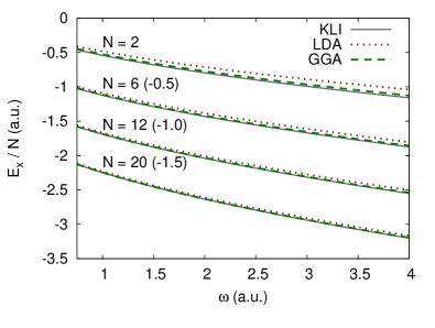
Figure 1: (color online) Exchange energy per electron for a series of parabolically confined quantum dots with $N$ electrons and confinement strength $\omega$. For clarity, the line for $N=6$ was shifted down by 0.5 a.u., the line for $N=12$ by 1 a.u., and the line for $N=20$ by 1.5 a.u. The lines are: exact exchange (solid gray), exchange-only LDA (dotted red), and this work (dashed green).

We can combine Eqs. (22) and (29) in an expression that interpolates the exchange energy of an inhomogeneous electron gas from the small density-gradient limit to the large one. A possible expression is of the form

$$E^{\rm GGA}_{\text{x}}[n_{\sigma},\nabla n_{\sigma}]=E^{\rm LDA}_{\text{x}}[n_{\sigma}]\\ -\beta\sum_{\sigma=\uparrow,\downarrow}\int\!\!{\rm d}^{2}r\>n^{3/2}_{\sigma}({\bf r})\frac{x^{2}_{\sigma}({\bf r})}{\left[1+\gamma x^{2}_{\sigma}({\bf r})\right]^{3/4}},$$ (31)

or, writing this expression explicitly in terms of the density and its gradients,

$$E^{\rm GGA}_{\text{x}}[n_{\sigma},\nabla n_{\sigma}]=E^{\rm LDA}_{\text{x}}[n_{\sigma}]\\ -\beta\sum_{\sigma=\uparrow,\downarrow}\int\!\!{\rm d}^{2}r\>\frac{|\nabla n_{\sigma}({\bf r})|^{2}}{n^{3/2}_{\sigma}({\bf r})\left[1+\gamma\frac{|\nabla n_{\sigma}({\bf r})|^{2}}{n^{3}_{\sigma}({\bf r})}\right]^{3/4}}\,,$$ (32)

where $\beta$ and $\gamma$ can be trivially written in terms of $\kappa_{\rm LGL}$ and $\kappa_{\rm SGL}$. At last, to improve the flexibility of the above approximate functional, we replace both $\beta$ and $\gamma$ with two parameters to be determined by fitting the exchange energies of an ensemble of physically relevant 2D systems.

We have chosen to fit our parameters to a set of four parabolic two-electron quantum dots qd with confinement stengths $\omega=1,\>1/4,\>1/16$, and 1/36 a.u., respectively. These are very well studied systems rontani that span a wide range of the density parameter, $0.9\lesssim r_{s}\lesssim 5.7$, where $r_{s}=N^{-1/6}\,\omega^{-2/3}$. For the reference exchange energies we performed self-consistent exact-exchange calculations with the code octopusoctopus using the Krieger-Li-Iafrate KLI (KLI) approximation, which is a very accurate approximation in the static case kli_oep . We obtained $\beta=0.003317$ and $\gamma=0.008323$, which are close to the parameters found by Becke for the 3D case by fitting a series of rare-gas atoms, $\beta^{\text{3D}}=0.00375$ and $\gamma^{\text{3D}}=0.007$ (Ref.  becke3, ).

Table 1: Exchange energies (in atomic units) for parabolic quantum dots. The last row contains the mean percentage error, $\Delta$. The first four lines represent the systems that were used in the fitting of $\beta$ and $\gamma$. The columns are: exact exchange (EXX), local density approximation (LDA), and the generalized gradient approximation presented in this work (GGA).

$N$	$\omega$	$-E^{\rm EXX}_{\rm x}$	$-E_{\rm x}^{\rm LDA}$	$-E_{\rm x}^{\rm GGA}$
2	1	1.083	0.9672	1.051
2	1/4	0.4850	0.4312	0.4704
2	1/16	0.2073	0.1843	0.2023
2	1/36	0.1239	0.1108	0.1276
6	0.42168	2.229	2.110	2.206
6	$1/1.89^{2}$	1.735	1.642	1.719
6	1/4	1.618	1.531	1.603
12	$1/1.89^{2}$	3.791	3.668	3.777
$\Delta$			7.9%	1.8%

Table 2: Exchange energies (in atomic units) for square (${\rm area}=\pi\times\pi$) quantum dots. The meaning of the columns is identical to Table 1.

$N$	$-E^{\rm EXX}_{x}$	$-E_{\rm x}^{\rm LDA}$	$-E_{\rm x}^{\rm GGA}$
2	1.417	1.288	1.383
6	6.147	5.902	6.180
8	9.509	9.017	9.434
12	16.24	15.91	16.46
16	25.23	24.35	25.15
$\Delta$		4.8%	1.1%

Our functional was then applied to parabolically confined quantum dots by varying the number of electrons $N$ in the dot and the confinement strength $\omega$. From the fully self-consistent DFT results summarized in Fig. 1 it is clear that our functional outperforms the LDA for the whole range of $N$ and $\omega$. A more quantitative picture can be obtained from Tables 1 and 2 where we present numerical values for the exchange energy obtained with different approximations, for both parabolically confined and hard-wall square square quantum dots, respectively. It is clear that our functional yields errors that are smaller by at least a factor of 4 than the errors of the simple LDA.

We tested the performance of our GGA functional also in the large-$N$ limit. Here we used the exact exchange energies known for parabolic closed-shell quantum dots of noninteracting electrons. zyl Using a fixed, analytic electron density as an input in Eq. (32), we found relative percentage errors of $0.7\,\%$ and $0.5\,\%$ for $N=110$ and $420$, respectively, whereas the corresponding errors of the LDA are $0.5\,\%$ and $0.2\,\%$. Even if the plain LDA is slightly more accurate in this case, we find the result very satisfactory in view of the fitting of $\beta$ and $\gamma$ according to two-electron data as explained above. We point out that in terms of potential applications for our GGA functional, the main interest is in relatively small systems (up to a few dozen of electrons). However, the GGA described here – possibly with simple modifications – enables precise many-electron calculations also in large-scale structures such as quantum-dot arrays zaremba or quantum-Hall devices. siddiki

IV Conclusions

We proposed a generalized gradient approximation for the exchange energy of two-dimensional systems, following the same lines developed for three-dimensional systems proposed by Becke becke2 ; becke3 . Analyzing the small- and large-density gradient limits, we arrived at the expression of a functional which depends on two parameters, that are fitted to a test set composed of four parabolically confined quantum dots containing two electrons. Further calculations, both for parabolically confined and square quantum dots, show that our approximations yields errors that are at least a factor of 4 better than the local density approximation.

We believe that this is the necessary step in the construction of reliable generalized gradient approximations for two-dimensional systems. The next steps will necessarily involve the construction of correlation functionals (beyond the local density approximation attaccalite or the forms proposed in Refs.  ususus, and  correlation, ), improvements to the exchange functional presented in this work, and further extensive tests, and analysis, to assess the quality of the same functionals. In this path we expect that the experience in the development of functionals in three dimensions will be a very useful guide, but we can also expect that experience gained in describing exchange and correlation in these low-dimensional systems can be again transposed to bring new insights and ideas into the three-dimensional world.

- (1) L. P. Kouwenhoven, D. G. Austing, and S. Tarucha, Rep. Prog. Phys. 64, 701 (2001); S. M. Reimann and M. Manninen, Rev. Mod. Phys. 74, 1283 (2002).
- (2) R. M. Dreizler and E. K. U. Gross, Density Functional Theory (Springer, Berlin, 1990).
- (3) A Primer in Density Functional Theory, edited by C. Fiolhais, F. Nogueira, and M. A. L. Marques (Springer-Verlag, Berlin, 2003).
- (4) U. von Barth, Phys. Scr. T109, 9 (2004).
- (5) J. P. Perdew and S. Kurth, in A Primer in Density Functional Theory, edited by C. Fiolhais, F. Nogueira, and M. A. L. Marques (Springer, Berlin, 2003), p. 1; G. E. Scuseria and V. N. Staroverov, in: Theory and Applications of Computational Chemistry: The First Forty Years, edited by C. E. Dykstra, G. Frenking, K. S. Kim, and G. E. Scuseria (Elsevier, Amsterdam, 2005), p. 669.
- (6) Y.-H. Kim, I.-H. Lee, S. Nagaraja, J.-P. Leburton, R. Q. Hood, and R. M. Martin, Phys. Rev. B 61, 5202 (2000).
- (7) L. Pollack and J. P. Perdew, J. Phys.: Condens. Matter 12, 1239 (2000).
- (8) A. K. Rajagopal and J. C. Kimball, Phys. Rev. B 15, 2819 (1977).
- (9) B. Tanatar, D. M. Ceperley, Phys. Rev. B 39, 5005 (1989).
- (10) C. Attaccalite, S. Moroni, P. Gori-Giorgi, and G. B. Bachelet, Phys. Rev. Lett. 88, 256601 (2002).
- (11) H. Saarikoski, E. Räsänen, S. Siljamäki, A. Harju, M. J. Puska, and R. M. Nieminen, Phys. Rev. B 67, 205327 (2003).
- (12) N. Helbig, S. Kurth, S. Pittalis, E. Räsänen, and E. K. U. Gross, Phys. Rev. B 77, 245106 (2008).
- (13) S. Pittalis, E. Räsänen, N. Helbig, and E. K. U. Gross, Phys. Rev. B 76, 235314 (2007)
- (14) E. Räsänen, S. Pittalis, C. Proetto, and E. K. U. Gross, submitted (arxiv:0807.1868)
- (15) S. Pittalis, E. Räsänen, and M. A. L. Marques, Phys. Rev. B 78, 195322 (2008).
- (16) S. Pittalis, E. Räsänen, C. Proetto, and E. K. U. Gross, submitted (arXiv:0810.4283).
- (17) J. P. Perdew, Phys. Rev. Lett. 55, 1665 (1985).
- (18) J. P. Perdew and Y. Wang, Phys. Rev. B 33, 8800 (1986).
- (19) A. D. Becke, Int. J. Quant. Chem. 23, 1915 (1983).
- (20) A. D. Becke, J. Chem. Phys. 85, 7184 (1986).
- (21) A. D. Becke, Phys. Rev. A 38, 3098 (1988).
- (22) U. von Barth and L. Hedin, J. Phys. C 5, 1629 (1972).
- (23) J. F. Dobson, J. Chem. Phys. 98, 8870 (1993).
- (24) E. Räsänen, A. Castro, and E. K. U. Gross, Phys. Rev. B 77, 115108 (2008).
- (25) P. Gori-Giorgi, S. Moroni, and G. B. Bachelet, Phys. Rev. B 70, 115102 (2004).
- (26) M. Brack and B. P. van Zyl, Phys. Rev. Lett. 86, 1574 (2001).
- (27) K. Berkane and K. Bencheikh, Phys. Rev. A 72, 022508 (2005).
- (28) M. Rontani, C. Cavazzoni, D. Bellucci, and G. Goldoni, J. Chem. Phys. 124, 124102 (2006).
- (29) M. A. L. Marques, A. Castro, G. F. Bertsch, A. Rubio, Comput. Phys. Commun. 151, 60 (2003); A. Castro, H. Appel, Micael Oliveira, C.A. Rozzi, X. Andrade, F. Lorenzen, M.A.L. Marques, E.K.U. Gross, and A. Rubio, Phys. Stat. Sol. (b) 243, 2465 (2006).
- (30) J. B. Krieger, Y. Li, and G. J. Iafrate, Phys. Rev. A 46, 5453 (1992).
- (31) T. Grabo, T. Kreibich, S. Kurth, and E. K. U. Gross, in Strong Coulomb Correlations in Electronic Structure Calculations: Beyond Local Density Approximations, edited by V. Anisimov (Gordon and Breach, Amsterdam, 2000); E. Engel, in A Primer in Density Functional Theory, edited by C. Fiolhais, F. Nogueira, and M. A. L. Marques (Springer-Verlag, Berlin, 2003).
- (32) E. Räsänen, H. Saarikoski, V. N. Stavrou, A. Harju, M. J. Puska, and R. M. Nieminen, Phys. Rev. B 67, 235307 (2003).
- (33) B. P. van Zyl, Phys. Rev. A 68, 033601 (2003).
- (34) See, e.g., B. P. van Zyl, E. Zaremba, and D. A. W. Hutchinson, Phys. Rev. B 61, 2107 (2000).
- (35) See, e.g., A. Siddiki and F. Marquardt, Phys. Rev. B 75, 045325 (2007) and references therein.