Lagrangian Structure Functions in Turbulence: Scaling Exponents and Universality

Abstract

In this paper, the approach for investigation of asymptotic ($Re\rightarrow\infty$) scaling exponents of Eulerian structure functions (J. Schumacher et al, New. J. of Physics 9, 89 (2007). ) is generalized to studies of Lagrangian structure functions in turbulence. The novel ”bridging relation” based on the derived expression for the fluctuating, moment-order - dependent dissipation time $\tau_{\eta,n}$, led to analytic expression for scaling exponents ($\kappa_{n}$ ) of the moments of Lagrangian velocity differences $S_{n,L}(\tau)=\overline{(u(t+\tau)-u(t))^{n}}\propto\tau^{\kappa_{n}}$ in a good agreement with experimental and numerical data.

Introduction. A turbulent flow can be described using Eulerian and Lagrangian approaches addressing dynamics of velocity field and evolution of individual fluid particles, respectively. Therefore, one can introduce two kinds of structure functions, i.e. moments of velocity increments. The properties of Eulerian correlation functions (ESF) were first theoretically investigated by Kolmogorov in his celebrated K41 theory of turbulence based on an exact in the inertial range relation for the third-order structure function $S_{3}(r)=\overline{{\bf(u(x+r)-u(x))}\cdot\frac{{\bf r}}{r})^{3}}\equiv\overline{({\bf\delta_{r}u}\cdot\frac{{\bf r}}{r})^{3}}\propto r$ [1]. The problem of Lagrangian correlation functions, for which not a single exact dynamic relation exists, is not new and was originally formulated within the framework of Kolmogorov theory of turbulence (for a detailed review, see Ref.[2]). Due to technological limitations of the past, experimental studies of strong turbulence were mainly devoted to Eulerian structure functions (ESF) $S_{n}=\overline{(u(x+r)-u(x))^{n}}\equiv\overline{(\delta_{r}u)^{n}}$ limited to the single- point measurements with subsequent application of Taylor hypothesis. Here $u$ is a component of velocity field parallel to the displacement vector ${\bf r}$ chosen along the $x$-axis. The experimental and numerical studies of Eulerian structure functions revealed two distinct intervals: while in the analytic range $r\rightarrow 0$ (or $r\ll\eta_{n}$), the velocity field is differentiable and $S_{n}(r)\propto r^{n}$, at the scales $L\gg r\gg\eta_{n}$, the ESFs are given by algebraic relations $S_{n}(r)\propto r^{\xi_{n}}$ with ‘anomalous’ scaling exponents $\xi_{n}$. By this definition, $\eta_{n}$’s are the cut-offs separating analytic and ‘rough’ ranges of ESFs. (See Fig.1).

The remarkable breakthroughs in experimental particle tracking, led by the Bodenschatz group [3]-[7], enabled investigation of Lagrangian structure functions (LSF) $S_{n,L}=\overline{(u(t+\tau)-u(t))^{n}}\equiv\overline{(\delta_{\tau}u)^{n}}$ which are a crucial ingredient in understanding of turbulent transport and mixing. Due to analyticity of velocity field, as $\tau\rightarrow 0$, $\delta_{\tau}u\approx a\tau$ where $a$ is acceleration of a fluid particle and $S_{nL}=\overline{a^{n}}\tau^{n}$. For the time-increments $\tau\gg\tau_{\eta,n}$, the LSFs $S_{nL}\propto\tau^{\kappa_{n}}$ with the dissipation times $\tau_{\eta,n}$ separating analytic and rough intervals on a time-domain. (See Fig.1). The recent multifractal theory of LSFs [6] stressed the importance of the dissipation time $\tau_{\eta}$ which was treated in the spirit of Kolmogorov theory as a moment-number- independent quantity $\tau_{\eta}\propto T/\sqrt{Re}=const$ where $T\approx L/u_{rms}$ is a large-scale eddy turn-over time. To make a connection between ESFs and LSFs, the authors of Ref. [6] used the ”bridging relation” (BR): $r\approx\tau\delta_{\tau}u\equiv\tau(u(t+\tau)-u(t))$ with the time-increment $\tau$ approximately equal to the fluctuating eddy turn-over time in the inertial range. This expression, introduced on dimensional grounds in Ref.[8], can be understood as follows. Consider a fluid particle at a time $t=t_{0}$ occupying position ${\bf X}_{0}$. Then, the particle displacement is: ${\bf R}={\bf X}(t_{0}+\tau)-{\bf X}_{0}=\int_{t_{0}}^{t_{0}+\tau}{\bf u}(\lambda)d\lambda$, so that ${\bf R}={\bf u}(t_{0})\tau+\int_{t_{0}}^{t_{0}+\tau}({\bf u}(\lambda)-{\bf u}(t_{0}))d\lambda$. We can see that if ${\bf u}(t)={\bf U}=const$, the displacement ${\bf R}\neq 0$. Then, following [2] (page 342, where it is related to transition to a moving frame of reference), we define the regularized (not involving single-point- velocity) quantity: ${\bf r}={\bf R}-{\bf u}(t_{0})\tau$. (It is estimated in Ref.[2] (page 359) that $r\approx 0$, meaning that it tends to zero when either $u\rightarrow U=const$ or $\tau\rightarrow 0$.) From the mean value theorem we also have $\int_{t_{0}}^{t_{0}+\tau}u(\lambda)d\lambda\approx u(t+\overline{\tau})\tau$, where $0<\overline{\tau}\leq\tau$. The relation $r\approx\tau\delta_{\tau}u$ is obtained in the first approximation setting $u(t+\tau)\approx u(t+\overline{\tau})$ which resembles the one used in construction of Kraichnan’s Lagrangian History Direct Interaction Approximation [9]. Keeping in mind topological complexity of developed turbulence, we conclude that the mean value theorem, leading to the ”bridging relation” $r\approx\tau\delta_{\tau}u$ with the inertial range time-increments $\tau\gg\tau_{\eta}$, cannot be accurate. Recently, the BR was analyzed using the exact relations between Eulerian and Lagrangian structure functions by Kamps et al [10] who showed that, combined with the multifractal formalism, it leads to the Lagrangian exponents in a substantial disagreement with experimental [3]-[7] and numerical [11] data. Moreover, it was pointed out that the theory of Ref. [6], expressing anomalies of Lagrangian exponents in terms of anomalies of Eulerian ones, does not explain the ”2D-paradox”: while the two-dimensional Eulerian turbulence is not intermittent, the Lagrangian one is.

In this paper, based on the ideas developed in Refs.[12]-[16], we attack the problem differently. In the analytic (dissipation) range where $\delta_{\tau}u\approx a\tau$, the displacement $r\approx\tau\delta_{\tau}u/2$. Extrapolating this to the dissipation cut-off $\eta$, separating analytic and rough intervals of the structure functions, leads to the dissipation time $\tau_{\eta}$ :

$$\eta\approx\tau_{\eta}\delta_{\tau_{\eta}}u$$ (1)

Both $\eta\approx\frac{\nu}{\delta_{\eta}u}$ and $\tau_{\eta}$ in formula (1) are random functions investigated in great detail theoretically and numerically [13]-[16]. Unlike the BR defined for the large inertial range values of the time - increment $\tau\gg\tau_{\eta}$, the expression (1), introduced as an extrapolation of the exact in the analytic interval relation, is accurate for short times $\tau\leq\tau_{\eta}$. Theoretical basis for this extrapolation is understood as follows. The structure functions, both Eulerian and Lagrangian, can be formally represented as $\psi_{n}(x)\propto x^{\beta_{n}(x)}$ with the $x$-dependent exponents $\xi_{n}\leq\beta_{n}(x)\leq n$ (or $\kappa_{n}\leq\beta_{n}(x)\leq n$) covering both analytic ($\beta_{n}=n$) and inertial ( $\beta_{n}(x)=\xi_{n}$ or $\beta_{n}=\kappa_{n}$) ranges. The smallest inertial range exponents giving maximum values to the differences $n-\beta_{n}$, correspond to the strongest singularities of velocity field and defining the cut - offs by the matching relation $\overline{a^{n}}\tau_{\eta,n}=K_{n}\tau_{\eta,n}^{\kappa_{n}}$, we account for the strongest, dominant, singularities. (See Ref.[16]).

Figure 1: Definition of the cut-off $\eta_{n}$ ( or $\tau_{\eta_{n}}$) for a structure function $S_{n}(x)$ (or$(S_{n,L}(x)$). As an example $S=S_{8}$ is chosen. The strait lines are $x^{8}$ (analytic range) and $x^{2.2}$ (inertial one). The point of their crossing is $x_{n}=\eta_{n}$. Schematic.

The probability distribution functions $Q(\eta,Re)$, derived and investigated numerically in [14]-[15] enable one to evaluate the moments of the dissipation scales:

$$\eta_{n}^{n}=\overline{\eta^{n}}=\int\eta^{n}Q(\eta,Re)d\eta\approx LRe^{\frac{n}{\xi_{n}-\xi_{n+1}-1}}$$ (2)

Combining (1) and (2) and assuming continuity of $S_{nL}(\tau)$ on the dissipation time scale yields:

$$L^{n}Re^{\frac{n}{\xi_{n}-\xi_{n+1}-1}}=(u_{rms}T)^{n}(\frac{\tau_{\eta,n}}{T})^{\kappa_{n}+n}$$ (3)

Our goal now is to express the dissipation times $\tau_{\eta,n}\equiv\tau_{n}$ in terms of the Reynolds number and, comparing the result with formula (2), obtain expressions for Lagrangian exponents $\kappa_{n}$.

Eulerian structure functions. Since energy dissipation in the inertial range dynamics ( inverse-energy-cascade ) of 2D turbulence is irrelevant, the relation (2), obtained by balancing viscous dissipation and inertial-range contributions to the exact equations for the Eulerian structure functions (see Refs. [14]-[16]) is valid for three-dimensional flows only. If, in accord with Kolmogorov theory, we assume $\xi_{n}=n/3$, this formula gives the well-known $n$-independent relation $\eta_{n}\approx LRe^{-\frac{3}{4}}$. However, due to intermittency, the function $\xi_{n}$ is a convex function of the moment order $n$ and for a fixed Reynolds number $Re=const$, the dissipation scales $\eta_{n}$ decrease with $n$. (This result has been numerically tested in Ref.[16]). Since the inertial range is compressed to the interval between integral and dissipation scales ($\eta_{n}\ll r\ll L/10$), experimental determination of exponents $\xi_{n}$ is very difficult and at the present time only the exponents $\xi_{n}$ with $n\leq 8$ have been accurately established by direct investigation of inertial range dynamics. In accord with the recently developed theory of small-scale intermittency, the dissipation scale is defined by a dynamic Reynolds number $Re_{\eta}=\frac{\eta\delta_{\eta}u}{\nu}\approx 1$ [15]. First, we see that the dissipation scale is not a constant as in K41, but a fluctuating property of a flow. Then, it is easy to show [14[-[16] that $\frac{\partial u}{\partial x}=\frac{\delta_{\eta}u}{\eta}\approx\frac{(\delta_{\eta}u)^{2}}{\nu}$. Since $\eta$ is the scale separating analytic and rough scale- intervals of the velocity field, it has been shown that:

$$\overline{(\frac{\partial u}{\partial x})^{n}}\approx S_{2n}(\eta_{2n})/\nu^{n}\propto\eta_{2n}^{\xi_{2n}}/\nu^{n}\propto Re^{\rho_{n}}$$ (4)

Using (2) we derive readily:

$$\rho_{n}=n+\frac{\xi_{2n}}{\xi_{2n}-\xi_{2n+1}-1};~{}d_{n}=n+\frac{\xi_{4n}}{\xi_{4n}-\xi_{4n+1}-1}$$ (5)

where $d_{n}$ are the exponents of the moments of the dissipation rate $\overline{{\cal E}^{n}}\approx\frac{\overline{(\delta_{\eta}u)^{4}}}{\nu}=S_{4n}(\eta_{4n})/\nu\propto Re^{d_{n}}$. According to this calculus, the moments of Lagrangian acceleration

$$\overline{a^{n}}=\overline{(\frac{(\delta_{\eta}u)^{3}}{\nu})^{n}}\propto Re^{\frac{\xi_{3n}}{\xi_{3n}-\xi_{3n+1}-1}+n}\equiv Re^{\alpha_{n}}$$ (6)

The quantitative results of Ref. [16], obtained with the help of a particular parametrization (Ref.[13]-[15])

$$\xi_{n}=0.383n/(1+n/20)$$ (7)

The predicted in Refs. [13]-[16] relations (4),(5) have been confirmed in the most detailed numerical simulation of Ref.[16] and [17]. The expression (7), calibrated to give $\xi_{3}=1$, is the result of a theory valid for the even - order moments only. We do not have any reason to believe that $\overline{|\delta_{r}u|^{3}}\propto r^{\xi_{abs}}$ with $\xi_{abs}=1$. Thus, the accuracy of the relation (7) must be of the order $|\xi_{3}-\xi_{3,abs}|$, which is numerically small. This drawback is common to all exisitng models leading to expression for $\xi_{n}$.

Lagrangian structure functions. The classical treatment of the problem can be formulated as follows [2]. As $\tau\rightarrow 0$, the velocity field is differentiable and using (6):

$$S_{2n,L}(\tau)=\overline{(\delta_{\tau}u)^{n}}=\overline{a^{2n}}\tau^{2n}\propto Re^{\alpha_{2n}}\tau^{2n}$$ (8)

The limit $\tau\rightarrow 0$, means that there exist a time-scale $\tau_{\eta,2n}$ such that the relation (8) is valid in the interval $\tau\ll\tau_{\eta,2n}$. In the ”inertial range $\tau_{\eta,2n}\ll\tau\ll T=\frac{1}{u_{rms}^{2}}\int_{t_{0}}^{t_{0}+\tau}\overline{u(0)u(t)}dt$, the velocity field is not differentiable and

$$S_{2n,L}(\tau)\propto\tau^{\kappa_{2n}}$$ (9)

In what follows we define n^th dissipation time $\tau_{2n}$ by the matching relation:

$$S_{2n,L}(\tau_{2n})=\overline{a^{2n}}\tau_{2n}^{2n}=({\cal E}\tau_{2n})^{n}(\frac{\tau_{2n}}{T})^{\kappa_{2n}-n}$$ (10)

According to K41, neither integral scale nor viscosity influence the dynamics of inertial range and, on dimensional grounds $\kappa_{2n}=n$ and $S_{2n,L}=K_{2n}({\cal E}\tau)^{n}$ with $K_{n}=const.$ Let us examine consistency of this result with some other predictions of the K41. It is clear that: $S_{2,L}=\int_{0}^{\tau}\int_{0}^{\tau}\overline{a(\lambda_{1})a(\lambda_{2})}d\lambda_{1}d\lambda_{2}$. By the time-homogeneity $\overline{a(\lambda_{1})a(\lambda_{2})}=A(\lambda_{1}-\lambda_{2})\equiv A(s)$ and

$$S_{2,L}=\int_{0}^{\tau}(\tau-s)A(s)ds$$ (11)

According to K41 (see Ref.[2]), in the interval $0<\tau<\tau_{\eta,2}$, $A(\tau)\approx\overline{a^{2}}$ and for $\tau_{\eta,2}<\tau\ll T$, $A(\tau)\approx K_{2}{\cal E}/\tau$. Substituting this into (11) gives the inertial range expression ($\tau\geq\tau_{\eta,2}$)

$$S_{2,L}(\tau)\approx\frac{\overline{a^{2}}\tau_{2}^{2}}{2}+K_{2}{\cal E}(\tau\ln\frac{\tau}{\tau_{2}}-\tau+\tau_{2})$$ (12)

We can notice a slight inconsistency of K41: the expressions (12) and the K41 result $S_{2,L}\propto\tau$ differ by a large logarithmic factor which is impossible to derive from dimensional considerations. Dimensional considerations [2] also give $\overline{a^{2}}\approx{\cal E}^{\frac{3}{2}}/\sqrt{\nu}\propto\frac{u_{rms}^{4}}{L^{2}}\sqrt{Re}$ and up to logarithmic correction, the second contribution to the right side of (12) is $O(1)$. Demanding continuity of the structure function $S_{n,L}$ in the limit $Re\rightarrow\infty$, we obtain the familiar K41 estimate for the relaxation time $\tau_{2}\approx\frac{u_{rms}}{a_{rms}}\propto Re^{-\frac{1}{2}}$. Accounting for intermittency. Since, $T\approx L/u_{rms}$ , then, as follows from (10), on the dissipation time-scale:

$$s_{2n}(\tau_{2n})=\frac{S_{2n,L}(\tau_{2n})}{u_{rms}^{2n}}=Re^{\alpha_{2n}}(\frac{\tau_{2n}}{T})^{2n}=K_{2n}(\frac{\tau_{2n}}{T})^{\kappa_{2n}}$$ (13)

and for $\tau\ll\tau_{2n}$:

$$S_{2n,L}\propto Re^{\alpha_{2n}}\tau^{2n};\hskip 14.22636pt\frac{\tau_{2n}}{T}\approx Re^{\frac{\alpha_{2n}}{\kappa_{2n}-2n}}\equiv Re^{-\gamma_{2n}}$$ (14)

Now, we derive the expression for $\kappa_{n}$. Combining (2),(3) with (14) gives:

$$L^{n}Re^{\frac{n}{\xi_{n}-\xi_{n+1}-1}}=(u_{rms}T)^{n}(\frac{\tau_{n}}{T})^{\kappa_{n}+n}=$$

$$(Tu_{rms})^{n}Re^{\frac{\alpha_{n}(\kappa_{n}+n)}{\kappa_{n}-n}}$$ (15)

and

$$\frac{n}{\xi_{n}-\xi_{n+1}-1}=\frac{\alpha_{n}(\kappa_{n}+n)}{\kappa_{n}-n}$$ (16)

n	$\xi_{n}$	$\alpha_{n}$	$\kappa_{n}^{th}$	$\kappa_{n}^{exp}$	$\gamma_{n}$
2	0.7	0.55	0.95	0.9-1. [4]’[10[,[11]	0.545
4	1.27	1.5	1.44	1.3-1.6 [2],[4],[5],[11]	0.566
6	1.77	2.6	1.74	1.6-1.8 [2],[4],[5],[11]	0.61
8	2.2	3.9	1.92	1.9,[4]	0.66
10	2.55	5.8	2.05	2.1, [4]	0.76

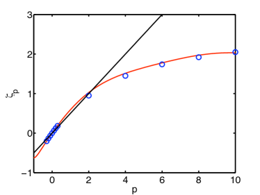
Figure 2: Top curve: Lagrangian and Eulerian exponents $\kappa_{n}$ and $\xi_{n}$ vs. $n$. Lagrangian ones are ”more intermittent”. Bottom: comparison of predicted (formula (14)) and experimentally observed exponents $\kappa_{p}\equiv\zeta_{p}$ [4]. Black line is exponents based on K41.

With the parametrization (7) (or any other, for that matter) one is able to calculate the exponents $\kappa_{n}$ of Lagrangian structure functions. The theoretical predictions ($\kappa_{n}^{th})$ are favorably compared with experimental and numerical ($\kappa_{n}^{exp})$ results in the Table.

The moment-number dependence of Lagrangian and Eulerian exponents is presented on Fig.2 (top curve) together with comparison of theoretical predictions with experimental data of Ref. [4].

The non-trivial Reynolds number dependence of the relaxation times $\tau_{\eta,n}$, given by expression (14), is also of importance. Plotting the experimental data on $S_{n,L}(\tau)$ in coordinates $\tau/\tau_{K}\approx T/\sqrt{Re}$ instead of $\tau/\tau_{n}$, the authors of Ref. [7] failed to collapse the experimental graphs for $S_{nL}(\tau,Re)$, which indicated a dynamic inconsistency of Kolmogoorv’s dissipation time. Similar phenomenon was described in Schumacher et. al. (Ref.[16]) dealing with the moments of increments Eulerian velocity field.

Conclusions. In this paper we used the theoretically predicted and experimentally verified fact [16] that the inertial-range asymptotic exponents of Eulerian structure functions are closely related to the anomalous Reynolds -number- scaling of the moments of velocity derivatives defined on the fluctuating ultra-violet cut-offs given by expression (2). Following [15],[16], we introduced the moment-number-dependent dissipation time which, combined with the new ”bridging relation” $\eta\approx\tau_{\eta}\delta_{\tau_{\eta}}u$, enabled us to evaluate the scaling exponents of Lagrangian structure functions in a good agreement with experimental and numerical data. Unlike the previously used BR, defined for the inertial range increments $\tau\gg\tau_{\eta}$, this relation, which is an extrapolation of an exact in the analytic range dependence $r=\tau\delta_{\tau}u/2$, is much more accurate.

I am grateful to Rainer Grauer for bringing my attention to the ”2D-paradox” and for many illuminating discussions. Working on this paper I, as always, benefited from the evergreen volumes by A.S. Monin and A.M. Yaglom. Sadly, this time I was unable to discuss all this with Akiva Moiseevich whom we lost in the fall of 2007. Most interesting and stimulating discussions with E. Bodenschatz, L. Biferale, Haitao Xu, K.R. Sreenivasan, and J. Schumacher are gratefully acknowledged.

References

1.  A.N. Kolmogorov, Dokl. Akad. Nauk SSSR 30, 299 (1941).
2. A.S. Monin and A.M. Yaglom, Statistical Fluid Mechanics, vol. 2 1975, MIT Press, Cambridge, MA
3. A. LaPorta et. al., Nature, London 409, 1017 (2001).
4. H. Xu, N. Ouelette and E. Bodenshcatz, Phys.Rev.Lett., 96, 024503 (2006); 5. M. Mordant, P. Metz, O. Michel and J.-F. Pinton, Phys.Rev.Lett. 87, 214501 (2001).
6. A. Arneodo et. al., Phys.Rev.Lett. 100, 254504 (2008.)
7. L. Biferale, E. Bodenschatz, M. Cencini, A.S. Lanotte, N.T. Oulette, F. Toschi, H. Xu, Phys. Fluids 20, 065103 (2008)
8. M.S. Borgas, Phil. Trans. R. Soc. A 342, 379 (1993); G. Boffetta, F. De Lillo, and S. Musacchio, Phys. Rev. E 66, 066307 (2002);
9. R. H. Kraichnan, Phys. Fluids 8, 575 (1965).
10. O.Kamps, R. Friedrich and R. Grauer, arXiv:0809.4339[physics.flu-dyn].
11. H. Homann, R. Grauer, A. Busse and W.C. Muller, J.Plasma Phys. 73, 821 (2007).
12. G. Paladin and A. Vulpiani, ‘Anomalous scaling laws in multifractal objects’, Phys.Rep. 156, 147-225 (1987) .
Phys. Rep. 35 1971-1973 (1987);  M. Nelkin, Phys. Rev. A 42 7226 (1992);   U. Frisch and M. Vergassola, Europhys. Lett. 14 439 (1991).
13. V. Yakhot, ‘Pressure-velocity correlations and anomalous exponents of structure functions in turbulence’, J. Fluid Mech., 495, 135 (2003).
14. V. Yakhot and K.R. Sreenivasan, ‘Toward dynamical theory of multifractals in turbulence’, Physica A 343, 147-155. Physica A 343 147 (2004);  V. Yakhot, Physica D 215 166-174 (2006).
15. V. Yakhot, J. Fluid. Mech. 606, 325 (2008).
16. J. Schumacher, K.R. Sreenivasan and V. Yakhot, New. J. of Physics 9, 89 (2007).
17. D.A. Donzis, P.K. Yeung and K.R. Sreenivasan, Phys. Fluids, 20, 045108, (2008).