Galactic Nonlinear Dynamic Model

Abstract

We develop a model for spiral galaxies based on a nonlinear realization of the Newtonian dynamics starting from the momentum and mass conservations in the phase space. The radial solution exhibits a rotation curve in qualitative accordance with the observational data.

Keywords: Galactic Rotation Curves; Dark Matter; Mathematical Modeling.

PACS numbers: 95.35.+d, 02.90.+p

1 Introduction

Galactic rotation curves are one of the most important evidences favoring the dark matter scenario in astrophysics. Actually dark matter was proposed by Zwicky [1] in order to accommodate observed velocities in galaxies and galaxy clusters. Since then others explanations was proposed as modifications of Newtonian gravity [2] or modifications in General Relativity [3]. All these approaches have in common, from the modeling point of view, just one element: non-linearity. So, is natural asks the question if non-linear effects of some sort are responsible for the discrepancy observed in galaxies and galaxy cluster dynamics. Recently, in the context of General Relativity, some authors have investigated this point [4].

Here, we will propose an alternative paradigm where Newtonian gravity is maintained on its solid basements but a non-linear model of a galaxy is build. We solve the non-linear equations in two simplified cases and calculate the resulting galaxy rotation curves, showing qualitatively that flat curves can be obtained in a given region of the parameter space.

2 The General Model

We focus on spiral galaxies described as a fluid with mass distribution in the phase space, $\Psi\left(\mathbf{x},\mathbf{v},t\right)$ which is related to the ordinary mass distribution by

$$\rho\left(\mathbf{x},t\right)=m_{\ast}\int d\mathbf{v~{}}\Psi\left(\mathbf{x},\mathbf{v},t\right)$$

where $m_{\ast}$ the mass for a typical star. the dynamics is governed by the Poisson equation coming from the second Newton law,

$$\mathbf{\nabla}^{2}V\left(\mathbf{x},t\right)=4\pi G\rho\left(\mathbf{x},t\right)$$

but restricted to the mass conservation,

$$\frac{d\Psi}{dt}=0\rightarrow\frac{\partial\Psi}{\partial t}+\frac{\partial\Psi}{\partial\mathbf{x}}\cdot\mathbf{\dot{x}}+\frac{\partial\Psi}{\partial\mathbf{v}}\cdot\mathbf{\dot{v}}=0$$

Using a Hamiltonian description, $\mathbf{\dot{x}=v}$, $\mathbf{\dot{v}}=-\mathbf{\nabla}V$, we obtain,

$$\frac{\partial\Psi}{\partial t}+\mathbf{v}\cdot\mathbf{\nabla}\Psi-\mathbf{\nabla}V\cdot\frac{\partial\Psi}{\partial\mathbf{v}}=0$$

$$\mathbf{\nabla}^{2}V\left(\mathbf{x},t\right)=4\pi G\int d\mathbf{v~{}}\Psi\left(\mathbf{x},\mathbf{v},t\right)$$

In general, this is a set of integro-differential non-linear coupled equations.

2.1 Axial Symmetry

Let us restrict the model only to the disc of the galaxy in the static regime. So, using the axial symmetry of this system, the mass conservation equation become:

$$\dot{r}\frac{\partial\Psi}{\partial r}+\dot{\phi}\frac{\partial\Psi}{\partial\phi}+\dot{z}\frac{\partial\Psi}{\partial z}-\left(\frac{\partial V}{\partial r}\frac{\partial\Psi}{\partial\dot{r}}+\frac{\partial V}{\partial\phi}\frac{\partial\Psi}{\partial\dot{\phi}}+\frac{\partial V}{\partial z}\frac{\partial\Psi}{\partial\dot{z}}\right)=0$$

This equation can be solved using the Method of Characteristics. Assuming a constant angular velocity, this is equivalent to a set of ordinary differential equations,

$$\frac{dr}{\dot{r}}=\frac{d\dot{r}}{-\frac{\partial V}{\partial r}}=\frac{dz}{\dot{z}}=\frac{d\dot{z}}{-\frac{\partial V}{\partial z}}~{},\;\frac{d\phi}{\dot{\phi}}=0~{},\;\frac{d\Psi}{dt}=0$$

whose uniparametric family of solutions is

$$\Psi=\Psi\left(E\right)~{},\;E=\frac{1}{2}\left(\dot{r}^{2}+r^{2}\dot{\phi}^{2}+\dot{z}^{2}\right)+V\left(r,z\right)$$

Experimental data shows that the mass distribution is Gaussian in the observed velocities, therefore is natural to choose the mass distribution $\Psi$ to be a Boltzmann distribution in the total energy:

$$\Psi\left(E\right)=\Psi_{0}e^{-\beta E}=\Psi_{0}\exp\left(-\beta\left[\frac{1}{2}\left(\dot{r}^{2}+r^{2}\dot{\phi}^{2}+\dot{z}^{2}\right)+V\left(r,z\right)\right]\right)$$

The integration over the velocities can be done, in order to obtain the functional dependence of the mass distribution over the gravitational potential

$$\rho\left(r,z\right)=\int d\dot{r}d\dot{\phi}d\dot{z}r\Psi\left(E\right)=\Psi_{0}\left(\frac{2\pi}{\beta}\right)^{3/2}\exp\left(-\beta V\left(r,z\right)\right)=\rho_{0}e^{-\beta V\left(r,z\right)}$$

It means that the Poisson equation now is a non-linear partial differential equation, given by

$$\frac{\partial^{2}V}{\partial r^{2}}+\frac{1}{r}\frac{\partial V}{\partial r}+\frac{\partial^{2}V}{\partial z^{2}}=4\pi G\rho_{0}e^{-\beta V\left(r,z\right)}$$

3 Variation in the Height

Let us to take an over simplified case, assuming that the field vary only with the height to the plane of the disc,

$$\frac{d^{2}V}{dz^{2}}=4\pi G\rho\left(z\right)=4\pi G\rho_{0}e^{-\beta V\left(z\right)}$$

Using an integration factor $\frac{dV}{dz}$ and the boundary conditions $V\left(0\right)=\frac{dV\left(0\right)}{dz}=0$ this equation can be directly integrated,

$$V\left(z\right)=\frac{2}{\beta}\ln\cosh\left(\frac{z}{z_{0}}\right)~{},\;z_{0}\equiv\left(2\pi G\rho_{0}\beta\right)^{-1/2}$$

The density profile in this case is

$$\rho\left(z\right)=\rho_{0}e^{-\beta V}=\frac{\rho_{0}}{\cosh^{2}\left(\frac{z}{z_{0}}\right)}$$

So far, it is a reasonable model, since the disc predicted is thin.

4 Radial Variation

Let us to take another over simplified model assuming variation only in the radial direction,

$$\frac{d^{2}V}{dr^{2}}+\frac{1}{r}\frac{dV}{dr}=4\pi G\rho_{0}e^{-\beta V\left(r\right)}$$

Multiplying both sides by $r$ and integrating, we find

$$r\frac{dV}{dr}-r_{0}c=4\pi G\rho_{0}\int_{r_{0}}^{r}\tilde{r}e^{-\beta V\left(\tilde{r}\right)}d\tilde{r}$$

where $r_{0}$ is the radius of the galaxy core, and $c\equiv\frac{dV\left(r_{0}\right)}{dr}$. Performing a second integration, we arrive in a Volterra second order integral equation:

$$V\left(r\right)=V_{0}+r_{0}c\ln\left(\frac{r}{r_{0}}\right)+4\pi G\rho_{0}\int_{r_{0}}^{r}d\bar{r}\int_{r_{0}}^{\bar{r}}\frac{\tilde{r}}{\bar{r}}e^{-\beta V\left(\tilde{r}\right)}d\tilde{r}$$

To solve it, we apply the Piccard’s method of successive approximations:

$$V^{\left(n+1\right)}\left(r\right)=V^{\left(0\right)}\left(r\right)+4\pi G\rho_{0}\int_{r_{0}}^{r}d\bar{r}\int_{r_{0}}^{\bar{r}}\frac{\tilde{r}}{\bar{r}}e^{-\beta V^{\left(n\right)}\left(\tilde{r}\right)}d\tilde{r}$$

$$V^{\left(0\right)}\left(r\right)=V_{0}+r_{0}c\ln\left(\frac{r}{r_{0}}\right)$$

Therefore, the first order iterative solution is

$$V^{\left(1\right)}\left(r\right) =V_{0}-4\pi G\rho_{0}e^{-\beta V_{0}}\left(\frac{r_{0}}{2-\beta r_{0}c}\right)^{2}+\left(r_{0}c-\frac{4\pi r_{0}^{2}G\rho_{0}e^{-\beta V_{0}}}{2-\beta r_{0}c}\right)\ln\left(\frac{r}{r_{0}}\right)+$$

$$+4\pi G\rho_{0}e^{-\beta V_{0}}\left(\frac{r}{2-\beta r_{0}c}\right)^{2}\left(\frac{r_{0}}{r}\right)^{\beta r_{0}c}$$

5 Galaxy Rotation Curve

Assuming a virial balance, $\frac{\upsilon^{2}}{r}=\frac{dV}{dr}\rightarrow\upsilon=\sqrt{r\frac{dV}{dr}}$, the galaxy rotation curve in this model is $\left(\bar{\beta}\equiv\beta r_{0}c~{},\;\left(r_{G}\right)^{-2}\equiv 4\pi G\rho_{0}~{},\;\lambda\equiv\frac{r}{r_{0}}~{},\;a\equiv\frac{r_{0}}{r_{G}}\right)$

$$\upsilon^{\left(1\right)}\left(\lambda\right)=\sqrt{\frac{\bar{\beta}}{\beta}+\left(\frac{a^{2}}{2-\bar{\beta}}\right)\left(\lambda^{2-\bar{\beta}}-1\right)}$$

In our illustrative example, $a=\beta=1$, we have the behavior illustrated in Fig. 1.

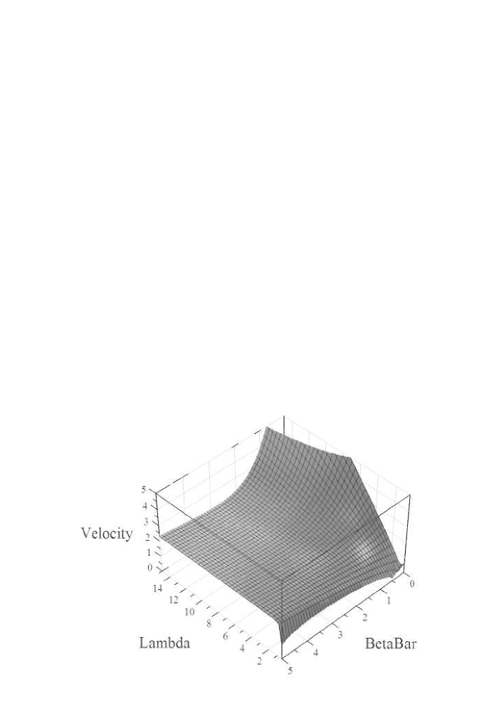
Figure 1: Parametric rotation curve. Velocity is given in units of $1/\beta^{1/2}$ and $\lambda$ is the distance to center in adimensional units. $\bar{\beta}$ is the parameter dictated by the boundary condition at the core.

So, if $\bar{\beta}>2$,

$$\lim_{\lambda\rightarrow\infty}\upsilon^{\left(1\right)}\left(\lambda\right)=\sqrt{\frac{\bar{\beta}}{\beta}-\left(\frac{a^{2}}{2-\bar{\beta}}\right)}$$

which is constant.

6 Final Remarks

A non-linear Newtonian model for the galaxy disk was constructed by introducing a solution of the mass conservation on the phase space.

We illustrate by a direct example that the non-linear character of the gravitational field is a key feature to understand galaxy rotation curves, even in the Newtonian case.

References

[1]F. Zwicky, Helv. Phys. Acta 6 (1933) 110.
[2]J. R. Bownstein and J. W. Moffat, Astrophys. J.636 (2006) ??; M. Milgrom, Astrophys. J.270 (1983)
365, ibid. 371, ibid. 384.
[3]S. Fay, Astron. Astrophys.413 (2004) 799;
S. Behar and M. Carmeli, Int. J. Mod. Phys.39 (2000) 1397;
S. Capozziello et al., Phys. Lett.A326 (2004) 292; D. N.
Vollick, Gen. Rel. & Grav.34 (2002) 471; K. Ichiki
et al., Phys. Rev. D66 (2002) 023514; R. R. Cuzinatto, C. A. M. de Melo, L. G. Medeiros and P. J.
Pompeia, Eur. Phys. J. C53 (2008) 98.
[4]M. D. Maia, A. J. S. Capistrano and D. Müller,
astro-ph/0605688.