Universal ratios of critical amplitudes in the Potts model universality class

Abstract

Monte Carlo (MC) simulations and series expansions (SE) data for the energy, specific heat, magnetization, and susceptibility of the three-state and four-state Potts model and Baxter-Wu model on the square lattice are analyzed in the vicinity of the critical point in order to estimate universal combinations of critical amplitudes. We also form effective ratios of the observables close to the critical point and analyze how they approach the universal critical-amplitude ratios. In particular, using the duality relation, we show analytically that for the Potts model with a number of states $q\leq 4$, the effective ratio of the energy critical amplitudes always approaches unity linearly with respect to the reduced temperature. This fact leads to the prediction of relations among the amplitudes of correction-to-scaling terms of the specific heat in the low- and high-temperature phases. It is a common belief that the four-state Potts and the Baxter-Wu model belong to the same universality class. At the same time, the critical behavior of the four-state Potts model is modified by logarithmic corrections while that of the Baxter-Wu model is not. Numerical analysis shows that critical amplitude ratios are very close for both models and, therefore, gives support to the hypothesis that the critical behavior of both systems is described by the same renormalization group fixed point.

The fixed points of the renormalization group define the universal behavior of a system through a set of critical exponents and universal combinations of critical amplitudes [1]. The universality concept divides all systems at criticality into a number of universality classes. It is instructive to know the set of values of the critical exponents and of the universal combinations of critical amplitudes for a given universality class.

The two-dimensional Potts model [2] is the simplest model which exhibits a phase transition. It is solved exactly at the critical point for any number of spin components $q$ and it is known that for $q\leq 4$ it has a continuous phase transition while for $q>4$ the phase transition is of the first order. The model has a great theoretical interest as new theories may be tested in this model.

At the same time, these models may have some practical interest as they may be realized in an adsorbate lattice placed onto a clean crystalline surface. The full classification of such systems with continuous transitions is known theoretically [3]. There are experiments in which some of them realize the 3-state and 4-state Potts models [4] and the critical exponents can be experimentally estimated.

Critical exponents for the Potts model with $q\leq 4$ can be computed exactly by different theoretical techniques [5, 6]. The values of the thermal critical exponents and of the magnetic critical exponents follow from the identification of the dimensions of the conformal algebra operators [6].

Nowadays, there is no doubt on the values of the leading critical exponents whereas the values of the correction-to-scaling exponents are still under discussion, as well as the values of the universal ratios of the critical amplitudes. Our presentation is intended to give a short review of the research on the subject.

The Potts model Hamiltonian [2] (see review [7] for details) can written as $H=-\sum_{\langle ij\rangle}\delta_{s_{i}s_{j}}\;,$ where $s_{i}$ is a spin variable taking integer values between $0$ and $q{-}1$, and the sum is restricted to the nearest neighbor sites $\langle ij\rangle$ on the square lattice.

Close to the critical temperature $T_{c}$ at which the continuous phase transition occurs, the residual magnetization $M$ and the singular part of the reduced susceptibility $\chi$ and of the specific heat $C$ of the system in zero external field are characterized by the critical exponents $\beta$, $\gamma$, and $\alpha$ and by the critical amplitudes $B$, $\Gamma_{\pm}$, and $A_{\pm}$

$$M(\tau) \approx B(-\tau)^{\beta},\ \tau<0$$ (1)

$$\chi_{\pm}(\tau) \approx \Gamma_{\pm}|\tau|^{-\gamma},$$ (2)

$$C_{\pm}(\tau) \approx \frac{A_{\pm}}{\alpha}|\tau|^{-\alpha},$$ (3)

where $\tau$ is the reduced temperature $\tau=(T-T_{c})/T$ and the labels $\pm$ refer to the high-temperature and low-temperature sides of the critical temperature $T_{c}$. The critical amplitudes are not universal by themselves but some combinations of them, f.e., $A_{+}/A_{-}$, $\Gamma_{+}/\Gamma_{-}$, and $\Gamma_{+}A_{+}/B^{2}$, are universal [1] due to the scaling laws.

On the square lattice, in zero field, the model is self-dual. The duality relation

$$\left(e^{\beta}-1\right)\left(e^{\beta^{*}}-1\right)=q$$ (4)

fixes the inverse critical temperature to $\beta_{c}{=}\ln(1{+}\sqrt{q})$. The values $E(\beta)$ and $E(\beta^{*})$ of the internal energy at dual temperatures are simply related through

$$\left(1-e^{-\beta}\right)E(\beta)+\left(1-e^{-\beta^{*}}\right)E(\beta^{*})=2.$$ (5)

Dual reduced temperatures $\tau$ and $\tau^{*}$ can be defined by $\beta{=}\beta_{c}(1{-}\tau)$ and $\beta^{*}{=}\beta_{c}(1{+}\tau^{*})$. Close to the critical point, $\tau$ and $\tau^{*}$ coincide through linear order, since $\tau^{*}{=}\tau{+}\frac{\ln(1{+}\sqrt{q})}{\sqrt{q}}\tau^{2}{+}O(\tau^{3})$.

The ratio of the free energy critical amplitudes $A_{+}/A_{-}$ is equal to unity due to duality. Moreover, duality relations may be used to understand the dependence on temperature of the effective amplitude functions which may be constructed from the energy in the symmetric phase $E_{+}(\tau)$ and in the ordered phase $E_{-}(\tau^{*})$

$$A_{+}(\tau) = \alpha(1-\alpha)\beta_{c}(E_{+}(\tau)-E_{0})\tau^{\alpha-1},$$ (6)

$$A_{-}(\tau^{*}) = \alpha(1-\alpha)\beta_{c}(E_{0}-E_{-}(\tau^{*}))(\tau^{*})^{\alpha-1}$$ (7)

as an effective amplitude ratio

$$\frac{A_{+}(\tau)}{A_{-}(\tau^{*})}=\frac{(E_{+}(\tau)-E_{0})\tau^{\alpha-1}}{(E_{0}-E_{-}(\tau^{*}))(\tau^{*})^{\alpha-1}},$$ (8)

where the constant $E_{0}$ is the value of the energy at the transition temperature, $E_{0}{=}E(\beta_{c}){=}{-}1{-}1/\sqrt{q}$.

Evaluating expression (8) for small $\tau$ and denoting $\alpha_{q}=-E_{0}\beta_{c}e^{-\beta_{c}}=\frac{\ln(1+\sqrt{q})}{\sqrt{q}}$, we obtain

$$\frac{A_{+}(\tau)}{A_{-}(\tau^{*})} = 1+(3-\alpha)\alpha_{q}\tau+O(\tau^{1+\alpha}).$$ (9)

Note the linear dependence on $\tau$ of the effective amplitude ratio.

The 2-state Potts model is equivalent to the Ising model which was solved exactly [8] (see Ref. [9] for details). The susceptibility behavior was understood in the paper by Wu, McCoy, Tracy and Barouch [10]. It turns out that there exist only integer corrections to scaling (for a recent and detailed discussions we refer readers to Refs. [11, 12, 13]). Values of the critical exponents and of some amplitude ratios are presented in Table 1.

Table 1: Exact values of critical exponents and ratios of critical amplitudes for the Ising model (2-state Potts model).

$\nu$	$\alpha$	$\beta$	$\gamma$	$A_{+}/A_{-}$	$\Gamma_{+}/\Gamma_{L}$	$R_{C}^{+}=\Gamma_{+}A_{+}/B^{2}$
1	0	$1/8$	$7/4$	1	37.69365…	0.318569…

The critical behavior of the susceptibility reads as

$$\chi(\tau)=\Gamma_{\pm}|\tau|^{-\gamma}{\cal X}_{corr}(|\tau|^{\Delta})+{\cal Y}_{bt}(\tau),$$ (10)

where ${\cal X}_{corr}(|\tau|^{\Delta})$ is the correction-to-scaling function and ${\cal Y}_{bt}(\tau)$ represents an analytic expression (“background term”) which accounts for non-singular contributions to susceptibility.

Set of values of the thermal critical exponents $x_{\epsilon_{n}}$ and of the magnetic critical exponents $x_{\sigma_{n}}$ are known analytically [5, 6]

$$x_{\epsilon_{n}}=\frac{n^{2}+ny}{2-y},\;\;\;x_{\sigma_{n}}=\frac{\left(2n-1\right)^{2}-y^{2}}{4(2-y)}$$ (11)

in terms of the variable $y$ linked to the number of states $q$ by $\cos\frac{\pi y}{2}=\frac{1}{2}\sqrt{q}$.

For the 3-state Potts model there is a finite number of correction terms [6], $x_{\epsilon_{2}}=14/5$, $x_{\epsilon_{2}}=6$, and $x_{\sigma_{2}}=4/3$. The leading correction-to-scaling contribution is $\Delta=-(2-x_{\epsilon_{2}})/(2-x_{\epsilon_{1}})=2/3$ and it was first supported in numerical simulation [14].

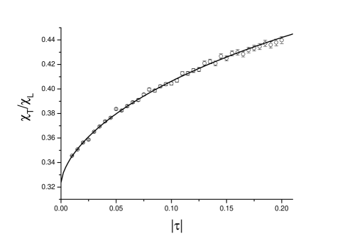
Figure 2: 3-state Potts model. Ratio of transverse to longitudinal susceptibilities.

Clear evidence for these leading correction to the scaling behavior may be seen in Figure 1, where we plot the difference of the longitudinal and transverse susceptibilities $(\chi_{L}-\chi_{T})$ (note the cancelation of background terms (10) in the difference) multiplied by the leading behavior factor $|\tau|^{\gamma}$, as a function of $|\tau|^{2/3}$. The ratio of the susceptibilities $(\chi_{T}/\chi_{L})$ is shown in Figure 2 and may be used to estimate the universal ratio of associated amplitudes $\Gamma_{T}/\Gamma_{L}$.

Analytical predictions for the amplitude ratios in Potts model for $q=2,3$, and 4 were given in the papers [15, 16]. The values are shown in the Table 2 together with numerical estimations from Monte Carlo (MC) and series expansions (SE) analyses [17, 18, 19]. The coincidence of the data is a good indication for the validity of both two-kink approximation [15, 16] to the exact scattering theory [20] for 3-state Potts model and of the analysis of MC data and series expansions.

Table 2: Exact values of critical exponents and estimates of the ratios of critical amplitudes for the 3-state Potts model.

$\nu$	$\alpha$	$\beta$	$\gamma$	$\Gamma_{+}/\Gamma_{L}$	$\Gamma_{T}/\Gamma_{L}$	$R_{C}^{+}{=}\Gamma_{+}A_{+}/B^{2}$	Remark
5/6	1/3	$1/9$	$13/9$	-	-	-	Exact result
				13.848	0.327	0.1041	[15, 16]
				13.83(9)	0.325(2)		[19] - SE
				13.83(9)	0.3272(7)	0.1044(8)	[18] - SE
				13.86(12)	0.322(3)	0.1049(29)	[18] - MC

The analysis of the 4-state Potts model is much more complicated because in addition to the corrections to scaling there are confluent logarithmic corrections [21, 22]. The result of the analysis of MC data and SE [23, 24, 19] is shown in the Table 3 together with the analytical estimates [15, 16].

Conformal field theory predicts the set of renormalization group (RG) exponents $y_{\epsilon_{n}}{=}2{-}x_{\epsilon_{n}}{=}$3/2, 0, -5/2, … . The leading correction-to-scaling exponent $y_{\epsilon_{2}}$ vanishes and gives rise to a logarithmic behavior [21]. In our recent publication [24, 25] we revised the renormalization group equations and included in our analysis the known form of the logarithmic corrections and of the next-to-leading corrections, taking into account the width of the temperature region window examined. The set of magnetic exponents for the Potts model $x_{\sigma_{n}}$=1/8, 9/8, 25/8, … translates into the magnetization exponent $\beta{=}1/12$ and the leading correction-to-scaling exponent $\Delta_{\sigma}{=}2/3$. Finally, the following behavior of the susceptibility is assumed

$$\chi_{+}(\tau)=\Gamma_{+}\tau^{-7/6}{\cal G}^{3/4}(-\ln\tau)(1+a_{+}\tau^{2/3}+b_{+}\tau)+D_{+},$$ (12)

where the function $\cal G$ contains a universal correction function $\cal E$ [22, 24, 25] and the leading nonuniversal correction function $\cal F$

$${\cal G}(-\ln|\tau|) = (-\ln|\tau|)\times{\cal E}(-\ln|\tau|)\times{\cal F}(-\ln|\tau|),$$ (13)

$${\cal E}(-\ln|\tau|) = \left(1+\frac{3}{4}\frac{\ln(-\ln|\tau|)}{-\ln|\tau|}\right)$$ (14)

$$\ \times\left(1-\frac{3}{4}\frac{\ln(-\ln|\tau|)}{-\ln|\tau|}\right)^{-1}\left(1+\frac{3}{4}\frac{1}{(-\ln|\tau|)}\right),$$

$${\cal F}(-\ln|\tau|) \simeq \left(1+\frac{C_{1}}{-\ln|\tau|}+\frac{C_{2}\ln(-\ln|\tau|)}{(-\ln|\tau|)^{2}}\right)^{-1}.$$ (15)

We fit our data to estimate the amplitude $\Gamma_{+}$, the coefficient of the leading correction to scaling $a_{+}$ in Eq. (12), and coefficients $C_{1}$ and $C_{2}$ in Eq. (15).

It is obvious that the logarithmic corrections (the whole function $\cal G(-\ln|\tau|)$) cancels in simple ratios, like $A_{+}/A_{-}$, $\Gamma_{+}/\Gamma_{L}$, $\Gamma_{T}/\Gamma_{L}$, etc. This has been demonstrated analytically for the effective ratio $A_{+}/A_{-}$ (see Eq. 9). We note also that the RG analysis predicts [24, 25] powers of logarithmic corrections to specific heat $\alpha^{\prime}{=}{-}1$, susceptibility $\gamma^{\prime}{=}3/4$, and magnetization $\beta^{\prime}{=}{-}1/8$ such that they cancel in all universal ratios. For example, the universal amplitude ratio $R_{C}^{-}$ may be calculated as the limit of the ratio of functions

$$R_{C}^{-}=\lim_{\tau\rightarrow 0}\tau\frac{(E_{-}(|\tau|)-E_{0})\chi_{-}(|\tau|)}{M(|\tau|)^{2}}\alpha(\alpha-1)\beta_{c}$$ (16)

where $E_{0}=E(0)=\sqrt{2}$. One can check that in the ratio (16) not only powers of $|\tau|$ cancel but also powers of $\cal E$. In the ratio, the magnetization $M$ and the energy difference $E_{-}(|\tau|)-E_{0}$ have only singular contributions and the only systematic deviation may come from the background correction to susceptibility $\chi_{-}(|\tau|)$. It was shown in [18] that the contribution from this background correction is negligible in the critical region window, and the estimator (16) tends to the value $0.0055(1)$ as $\tau\rightarrow 0$.

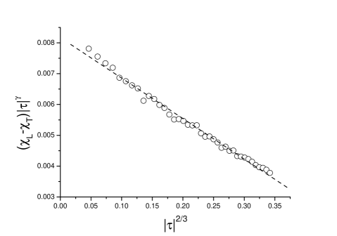
Figure 1: 3-state Potts model. Difference of susceptibilities $(\chi_{L}-\chi_{T})|\tau|^{\gamma}$ as function of $|\tau|^{2/3}$. The almost linear dependence supports the value 2/3 for the power of the leading correction to scaling.

The Baxter-Wu [26] model is defined on a triangular lattice, with spins $\sigma_{i}$ located at vertices. The three spins forming a triangular face are coupled with a strength $J$, and the Hamiltonian reads

$${\cal H}=-J\sum_{\rm faces}\sigma_{i}\sigma_{j}\sigma_{k},$$ (17)

where the summation extends over all triangular faces of the lattice, both pointing up and down. The ground state is four-fold degenerate and the critical exponents are found to be the same as for the 4-state Potts model.

The exact behavior of the magnetization, energy, and specific heat are known analytically [26, 27, 28]. An analysis of Monte Carlo data was performed by two of us [29] and preliminary estimates shows that the values of the susceptibility amplitude-ratio $\Gamma_{+}/\Gamma_{L}\approx 6.9$ and of the ratio $R_{C}^{-}\approx 0.005$ are very near to those obtained from our analysis of MC and SE data for the 4-state Potts model (see Table 3). We have to note that logarithmic corrections to scaling are absent in the critical behavior of Baxter-Wu model and this gives us more confidence in our analysis.

Delfino and Grinza [30] use the same analytical approach as in [15] to study the Ashkin-Teller model which also belongs to the 4-state Potts model universality class with some particular choice of coupling constants. This leads to the estimatation $\Gamma_{+}/\Gamma_{L}\approx 4.02$ and $\Gamma_{T}/\Gamma_{L}\approx 0.129$. This result is also very near to those for 4-state Potts model (see second entry in Table 3.)

A possible explanation of the deviation of our results from the analytical predictions may be explained as follows: the two-kink approximation is exact for the 2-state Potts model, it gives good accuracy for the 3-state Potts model, but it may be insufficient to produce accurate values for 4-state Potts model. Further analyses have to be done to resolve the contradiction among these results.

Table 3: Exact values of critical exponents and estimations of the ratios of critical amplitudes for the 4-state Potts model.

$\nu$	$\alpha$	$\beta$	$\gamma$	$\Gamma_{+}/\Gamma_{L}$	$\Gamma_{T}/\Gamma_{L}$	$R_{C}^{-}{=}\Gamma_{-}A_{-}/B^{2}$	Remark
2/3	2/3	$1/12$	$7/6$	-	-	-	Exact result
				4.013	0.129	0.00508	[15, 16]
				3.5(4)	0.11(4)		[19] - SE
				3.14(70)		0.0068(9)	[23] - MC
				6.93(6)	0.1674(30)	0.00512(13)	[24, 25] - MC
				6.30(1)	0.1511(24)	0.00531(5)	[24, 25] - SE

BB and WJ acknowledge partial support within the Graduate School “Statistical Physics of Complex Systems” of DFH-UFA under Contract No. CDFA-02-07. Financial support within a common research program between the Landau Institute and the Ecole Normale Supérieure de Paris, Paris Sud University is also gratefully acknowledged.

References

- [1] V. Privman, P.C. Hohenberg, A. Aharony, in Phase Transitions and Critical Phenomena, Vol. 14, edited by C. Domb and J.L. Lebowitz (Academic, New York, 1991).
- [2] R.B. Potts, Proc. Camb. Phil. Soc. 48 (1952) 106.
- [3] E. Domany, M. Schick, J. Walker, and R.B. Griffiths, Phys. Rev. B 18 (1978) 2209; E. Domany and M. Schick, Phys. Rev. B 20 (1979) 3828; C. Rottman, Phys. Rev. B 24 (1981) 1482.
- [4] A. Aharony, K. A. Muller and W. Berlinger, Phys. Rev. Lett. 38 (1977) 33;H. Pfnür and P. Piercy, Phys. Rev. B 41 (1990) 582; M. Sokolowski and H. Pfnür, Phys. Rev. Lett. 49 (1994) 7716; Y. Nakajima, et al, Phys. Rev. B 55(1997) 8129; C. Voges and H. Pfnür, Phys. Rev. B 57 (1998) 3345.
- [5] M.P.M. den Nijs, J. Phys. A 12 (1979)1857; R.B. Pearson, Phys. Rev. B 22 (1980) 2579; B. Nienhuis, J. Phys. A 15 (1982) 199; B. Nienhuis, J. Stat. Phys. 34 (1984) 731; B. Nienhuis, in Phase Transitions and Critical Phenomena,Vol. 11, edited by C. Domb and J.L. Lebowitz(Academic Press, London, 1987).
- [6] Vl.S. Dotsenko, Nucl. Phys. B 235 (1984) 54; Vl.S. Dotsenko and V.A. Fateev, Nucl. Phys. B 240 (1984) 312.
- [7] F.Y. Wu, Rev. Mod. Phys. 54 (1982) 235.
- [8] L. Onsager, Phys. Rev. ]65 (1944) 117.
- [9] B. M. McCoy and T.T. Wu, The two-dimensional Ising model (Harvard Uni. Press, Camdridge, Massachusetts, 1973)
- [10] E. Barouch, B.M. McCoy, and T.T. Wu, Phys. Rev. Lett. 31 (1973) 409; C.A. Tracy and B.M. McCoy, Phys. Rev. Lett. 31 (1973) 1500; T.T. Wu, B.M. McCoy, C.A. Tracy, and E. Barouch, Phys. Rev. B 13 (1976) 316.
- [11] Orrick, W. P., Nickel, B. G., Guttmann, A. J., and Perk, J. H. H., Phys. Rev. Lett. 86 (2001) 4120; J. Stat. Phys. 102 (2001) 795.
- [12] M. Caselle, M. Hasenbusch, A. Pelissetto, E. Vicari, J.Phys. A 35 (2002) 4861.
- [13] G. Delfino, Phys.Lett. B450 (1999) 196
- [14] G. von Gehlen, V. Rittenberg, and H. Ruegg, J. Phys. A 19 (1985) 107.
- [15] G. Delfino and J.L. Cardy, Nucl. Phys. B 519 (1998) 551.
- [16] G. Delfino, G.T. Barkema and J.L. Cardy, Nucl. Phys. B 565 (2000) 521.
- [17] L.N. Shchur, P. Butera, and B. Berche, Nucl. Phys. B 620 (2002) 579.
- [18] L.N. Shchur, L.N. Shchur, and P. Butera, Phys. Rev. B 77 (2008) 144410.
- [19] I.G. Enting and A.J. Guttmann, Physica A 321 (2003) 90.
- [20] L. Chim and A.B. Zamolodchikov, Int. J. Mod. Phys. A 7 (1992) 5317.
- [21] M. Nauenberg and D.J. Scalapino, Phys. Rev. Lett. 44 (1980) 837; J. L. Cardy, N. Nauenberg and D.J. Scalapino, Phys. Rev. B 22 (1980) 2560.
- [22] J. Salas and A. Sokal, J. Stat. Phys. 88 (1997) 567.
- [23] M. Caselle, R. Tateo, and S. Vinci, Nucl. Phys. B 562 (1999) 549.
- [24] L.N. Shchur, B. Berche and P. Butera, Europhys. Lett. bf 81 (2008) 30008.
- [25] L.N. Shchur, B. Berche and P. Butera, unpublished.
- [26] R. J. Baxter and F.Y. Wu, Phys. Rev. Lett. 31 (1973) 1294; Aust. J. Phys. 27 (1974) 357; R.J. Baxter, Aust. J. Phys. 27 (1974) 369.
- [27] R.J. Baxter, Exactly Solved Models in Statistical Mechanics (New York, Academic Press, 1982).
- [28] G.S. Joyce, Proc. R. Soc. Lond. A 343 (1975); ibid 345 (1975) 277.
- [29] L.N. Shchur and W. Janke, unpublished.
- [30] G. Delfino and P. Grinza, Nucl. Phys. B 682 (2004) 521.