Fermions and Loops on Graphs. II. Monomer-Dimer Model as Series of Determinants.

Abstract

We continue the discussion of the fermion models on graphs that started in the first paper of the series. Here we introduce a Graphical Gauge Model (GGM) and show that : (a) it can be stated as an average/sum of a determinant defined on the graph over $\mathbb{Z}_{2}$ (binary) gauge field; (b) it is equivalent to the Monomer-Dimer (MD) model on the graph; (c) the partition function of the model allows an explicit expression in terms of a series over disjoint directed cycles, where each term is a product of local contributions along the cycle and the determinant of a matrix defined on the remainder of the graph (excluding the cycle). We also establish a relation between the MD model on the graph and the determinant series, discussed in the first paper, however, considered using simple non-Belief-Propagation choice of the gauge. We conclude with a discussion of possible analytic and algorithmic consequences of these results, as well as related questions and challenges.

Gauge theories, stated in terms of fermions and gauge fields (e.g. associated with a vector potential), are common in theoretical and mathematical physics Polyakov (1987); Zinn-Justin (1989). Normally in physics, e.g. discussing quantum electrodynamics or quantum gravity, these popular theories are defined over continuous spaces, or their natural discretizations, e.g. triangulated Eucledian grids. In the discretized versions, e.g. in Lattice Gauge Theories Wilson and Kogut (1974), fermions are normally associated with vertexes of the grid, while gauge variables reside on edges.

In this paper we extend this standard discretized construction to arbitrary graphs and show that the gauge theory approach, native of physics, can be useful for getting new nontrivial relations between different graphical models that describe computer science problems defined on arbitrary graphs. We introduce and discuss a Graphical Gauge Model (GGM). Gauge fields in our construction correspond to standard binary variables, which could also be called Ising spins/variables, or more formally, the gauge group of the theory is $\mathbb{Z}_{2}$. Two objects emerging in any gauge theory, determinants and loops, are therefore natural participants of our description. We also find that this approach and language fits naturally with the Loop Calculus introduced in Chertkov and Chernyak (2006a, b) and extended in the first paper of the series Chernyak and Chertkov (2008) to the Gaussian Graphical models on graphs.

The power of GGM is in its natural operational flexibility: changing the order of integrations and modifying the integrand in the expression for the model’s partition function result in a variety of nontrivial relations, some of them discussed in this paper. Integration over the Grassman-fermion variables turns the partition function of GGM into a $\zeta$-function dependent on the gauge (binary variable) configuration. Here the $\zeta$-function is understood as a generating function for the expectation values of the Grassman variables and their combinations. In this formulation it is related to the inverse of the Ihara $\zeta$-function of the graph Ihara (1966).

Even though we are making a point in promoting the language of Grassman/fermion integration in this paper, and the series in general, our two main statements are made in terms of “normal” objects, e.g. determinants, disjoint oriented cycles, and also partition functions of the monomer-dimer model. Given that this latter object did not appear in the first paper of the series, we find it useful to state it casually right away (see the rhs of Eq. (6) for formal definition). Consider a graph, and cost functions, $w_{a}$ and $w_{ab}$, associated with the vertices and edges of the graph. A monomer-dimer configuration on the graph is a set of colorings of vertices and edges so that either any vertex of the graph is colored and then no adjusted edges are colored, or the vertex is not colored but then one of the adjusted edges is colored. The partition function of the monomer-dimer model on the graph is the sum over all allowed monomer-dimer configurations/colorings, where each individual contribution is a product of factors associated with colored vertices and edges over the graph . Armed with this definition let us now state the main results reported in the paper:

• The partition function, $Z_{MD}$, of the monomer-dimer model on a graph ${\cal G}$ is expressed in terms of a matrix $H$ built from the monomer and dimer weights placed at the diagonal and off-diagonal elements, respectively. Specifically, $Z_{MD}({\cal G})$ is stated as a series over the oriented disjoint cycles $C\in{\rm ODC}({\cal G})$ of the graph. An oriented disjoint cycle $C\in{\rm ODC}({\cal G})$ is represented by a disjoint union of simple oriented loops. Each term in the series is equal to the determinant of the original matrix $H$ with the cycles excluded, $H|_{{\cal G}\setminus C}$, multiplied by the product along the simple loops of the cycle of the corresponding off-diagonal elements taken with the reversed signs. (See Eqs. (6,15).)

• The determinant of $H$ is stated as a series over oriented disjoint cycles $C\in{\rm ODC}({\cal G})$ of the graph ${\cal G}$, where each term is equal to the partition function, $Z_{MD}({\cal G}\setminus C)$, of the monomer-dimer of the original graph with the cycle excluded, multiplied by the product along the simple loops of the cycle of the off-diagonal elements taken with the reversed signs. (See Eqs. (25,6).)

Three remarks are in order. First, the two main statements are equivalent, in fact, one is a kind of an inverse of the other (see Appendix A for clarifications). Second, the first statement has an immediate algorithmic consequence: it may be used for an approximate computation of the monomer-dimer partition function (which is known to be an $\#P$-complete, i.e. a counting problem of the likely exponential complexity Jerrum (1990)) via a truncation of the determinant series (the complexity of a determinant evaluation is cubic in the graph size). Third, the statement number two (expansion of the determinant in a series over oriented disjoint cycles) can be derived by implementing the Gauge fixing approach in the spirit of Chertkov and Chernyak (2006a, b), however selecting a gauge different from the Belief Propagation (BP) gauge. The latter resulted in the Loop Series expansion for the determinant, described in the first paper of the series Chernyak and Chertkov (2008).

A schematic set of relations between the two main statements and other results and models discussed in the paper, are shown in Fig. 1. The distribution of material is as follows. GGM is introduced in Section I.1. Direct relations between GGM and partition function of MD and DCS over determinants are established in Section I.2 and Section I.3 respectively. Inverse of the relation, expressing determinant as a series over partition functions of MD models on the original graph with disjoint cycles excluded is discussed in Section II, with some auxiliary material placed in Appendix A and Appendix B. Section III is reserved for Summary and Conclusions.

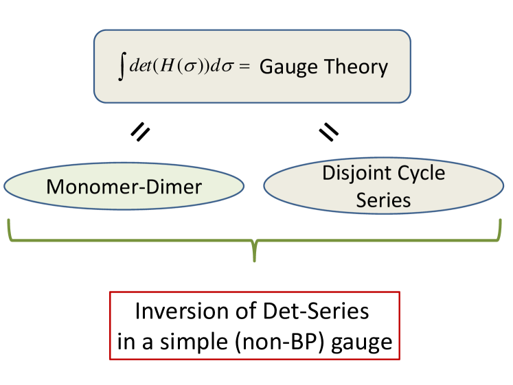
Figure 1: Schematic description of relations between models and concepts discussed in the paper.

I Graphical Gauge Model, Monomer-Dimer and Disjoint Cycle Series

I.1 Graphical Gauge Model

The determinant of a matrix was the key object discussed in Chernyak and Chertkov (2008). Thus, we naturally start a technical description in this second paper with stating a new model in terms of determinants.

Consider a square matrix, $H$, with elements $H_{ab}$, $a,b=1,\cdots,N$, and define a set of transformed (twisted) matrices, $H(\bm{\sigma})$, determined by a set of fields, ${\bm{\sigma}}=(\sigma_{ab}=\pm 1|a\neq b;\;a,b=1,\cdots,N)$, hereafter referred to as gauge fields, according to the following rule: $H_{ab}({\bm{\sigma}})=\sigma_{ab}H_{ab}$ and $H_{aa}({\bm{\sigma}})=H_{aa}$. The generalized $\zeta$-function of the matrix (understood as a generating function for Grassman variables correlations) is defined simply as the determinant,

$$\zeta({\bm{\sigma}})\equiv\det\left(H({\bm{\sigma}})\right).$$ (1)

Note that the Ihara $\zeta$-function of a graph depends on a spectral parameter represented by a complex number $\omega$. We add an additional set of binary spectral parameters, represented by the gauge field components and set $\omega=0$.

The matrix $H$ also defines an undirected graph ${\cal G}(H)$ with $N$ nodes $a\in{\cal G}_{0}$. The nodes $a$ and $b$ are connected by an edge $\alpha=\{a,b\}\in{\cal G}_{1}$ when $H_{ab}\neq 0$ or $H_{ba}\neq 0$. In other words the nodes $a\in{\cal G}_{0}$ represent the diagonal elements $H_{aa}$, whereas the edge $\{a,b\}\in{\cal G}_{1}$ corresponds to the pair of the off diagonal matrix elements $H_{ab}$ and $H_{ab}$ where at least one of the elements is nonzero. Hereafter we will also use a convenient notation $a\sim b$ for $\{a,b\}\in{\cal G}_{1}$. Note that for defining the $\zeta$-function we need only those components $\sigma_{ab}$ that are related to the edges of ${\cal G}$, i.e., $a\sim b$. Therefore, hereafter the gauge fields will include the relevant components, only, i.e. ${\bm{\sigma}}=(\sigma_{ab}=\pm 1|a\neq b;\;a\sim b;\;a,b=1,\cdots,N)$.

The last comment allows the configurations ${\bm{\sigma}}$ to be interpreted as discrete gauge fields with the gauge group $\mathbb{Z}_{2}$ that reside on the graph ${\cal G}$ in the full accordance with the terminology of the Lattice Gauge Theories Wilson and Kogut (1974); Polyakov (1987); Zinn-Justin (1989), originally developed in the context of regular lattices. Recall that in Lattice Gauge Theories the components $\sigma_{ab}$ of a gauge field reside on the edges of the lattice and take values in the gauge group; the latter means that in our case the gauge group is $\mathbb{Z}_{2}$. It is important to note that generally $\sigma_{ab}\neq\sigma_{ba}$, they rather satisfy the constraints $\sigma_{ba}\sigma_{ab}=1$ (with $1$ being naturally the gauge group unit element). However, in our special case of the $\mathbb{Z}_{2}$ gauge group the constraints imply $\sigma_{ba}=\sigma_{ab}$, and we can interpret the gauge field components as residing on the graph unoriented edges $\{a,b\}=\{b,a\}$, not on plaquettes as common in standard Lattice Gauge Theories considered on surface graphs .

The $\mathbb{Z}_{2}$ gauge theory associated with matrix $H$ and the graph ${\cal G}(H)$, respectively, is stated simply as an average/sum of the gauge-field-dependent determinant over all possible configurations of the gauge field on the graph. The partition function of the model becomes

$$Z=2^{-|{\cal G}_{1}|}\sum_{{\bm{\sigma}}\in{\cal G}_{1}}\zeta({\bm{\sigma}})\equiv\int_{{\cal G}_{1}}{\cal D}{\bm{\sigma}}\det(H({\bm{\sigma}})),$$ (2)

where the “integral” over the set of nonzero edges on the rhs is simply a convenient notation for the sum over $2^{|{\cal G}_{1}|}$ possible states of the discrete gauge fields and $|{\cal G}_{1}|$ stands for the cardinality of ${\cal G}_{1}$ (i.e., number of edges of ${\cal G}$).

Obviously one can think of any determinant on the rhs of Eq. (2) as of the one derived in the result of averaging/integration over Grassman variables ${\bm{\theta}}$, associated with the vertexes of ${\cal G}$. Adopting the notation introduced in the first paper Chernyak and Chertkov (2008) (see also Berezin (1987)) we can recast the partition function (2) in a form

$$Z=\int_{{\cal G}_{1}}{\cal D}{\bm{\sigma}}\int{\cal D}{\bm{\theta}}{\cal D}\bar{\bm{\theta}}\exp\left({\cal S}_{0}(\bar{\bm{\theta}},{\bm{\theta}};{\bm{\sigma}})\right),$$ (3)

$$S_{0}(\bar{{\bm{\theta}}},{\bm{\theta}};{\bm{\sigma}})=\sum_{a\in{\cal G}_{0}}H_{aa}\bar{\theta}_{a}\theta_{a}+\sum_{\{a,b\}\in{\cal G}_{1}}\sigma_{ab}(H_{ab}\bar{\theta}_{a}\theta_{b}+H_{ba}\bar{\theta}_{b}\theta_{a}).$$ (4)

Following the terminology commonly accepted in the field theory and mathematical physics we call $S_{0}$ the action of the Graphical Gauge Model. Note that, since the action in Eq. (4) depends on the gauge field ${\bm{\sigma}}$, it describes free fermions, interacting with the gauge field. The action of the pure gauge field in this model is zero.

I.2 Monomer-Dimer Model

The integrations/summations on the rhs of Eq. (3) obviously commutes, thus exchanging the order of integration, expanding vertex terms of the integrand in the series, utilizing the anti-commuting features of the Grassman variables and, finally, integrating over the binary gauge variables, one derives

$$\int_{{\cal G}_{1}}{\cal D}{\bm{\sigma}}e^{S_{0}(\bar{{\bm{\theta}}},{\bm{\theta}};{\bm{\sigma}})}=\prod_{a\in{\cal G}_{0}}(1+w_{a}\bar{\theta}_{a}\theta_{a})\prod_{\{a,b\}\in{\cal G}_{1}}(1+w_{ab}\bar{\theta}_{a}\theta_{a}\bar{\theta}_{b}\theta_{b}),$$ (5)

where $w_{ab}\equiv-H_{ab}H_{ba}$ and $w_{a}\equiv H_{aa}$. Expanding Eq. (5) into a polynomial and integrating the resulting expression over the Grassman variables we find that only terms associated with valid monomer-dimer configurations survive (are nonzero), i.e.

$$Z=Z_{MD}\equiv\sum_{\bm{\pi}}\left(\prod_{a\in{\cal G}_{0}}w_{a}^{\pi_{a}}\right)\left(\prod_{\{a,b\}\in{\cal G}_{1}}w_{ab}^{\pi_{ab}}\right)\left(\prod_{a\in{\cal G}_{0}}\delta\left(\pi_{a}+\sum_{b\sim a}\pi_{ab},1\right)\right),$$ (6)

where the set of ${\bm{\pi}}$ consists of two sub-sets of binary $0,1$ variables defined on the vertexes of the graph and on the edges of the graph, respectively: ${\bm{\pi}}\equiv{\bm{\pi}}_{v}\cup{\bm{\pi}}_{e}$, ${\bm{\pi}}_{v}\equiv(\pi_{a}=0,1;a\in{\cal G}_{0})$, and ${\bm{\pi}}_{e}\equiv(\pi_{ab}=0,1;\{a,b\}\in{\cal G}_{1})$. The last term on the rhs of Eq. (6) stated in terms of the Kroneker symbols describes the set of the monomer-dimer exclusions. In other words, a monomer-dimer configuration corresponds to a coloring of the graph (its vertexes and edges) in such a way that either at least one edge adjusted to the vertex is colored and then the vertex is not colored, or the adjusted vertexes are all uncolored and then the vertex is colored.

Note that Eq. (5) after some obvious modification can be viewed as a definition of an effective action $S(\bar{{\bm{\theta}}},{\bm{\theta}})$ that depends on the fermion variables only

$$\int_{{\cal G}_{1}}{\cal D}{\bm{\sigma}}e^{S_{0}(\bar{{\bm{\theta}}},{\bm{\theta}};{\bm{\sigma}})}=e^{S(\bar{{\bm{\theta}}},{\bm{\theta}})},\;\;\;S(\bar{{\bm{\theta}}},{\bm{\theta}})=\sum_{a\in{\cal G}_{0}}w_{a}\bar{\theta}_{a}\theta_{a}+\sum_{\{a,b\}\in{\cal G}_{1}}w_{ab}\bar{\theta}_{a}\theta_{a}\bar{\theta}_{b}\theta_{b},$$ (7)

As it usually happens in gauge theories, integration over the gauge field creates fermion interactions (second term in the action in Eq. (7)). The interaction can be decoupled by introducing a Hubbard-Stratonovich field represented by another $\mathbb{Z}_{2}$ gauge field coupled to $\theta_{a}\theta_{b}$ and $\bar{\theta}_{a}\bar{\theta}_{b}$. This results ina representation of the partition function of the Monomer-Dimer model in a form of an integral (sum) over the gauge field, with the integrand represented as a product of two gauge-field dependent Pfaffians. This representation will be studied in detail in the next paper of the series, with the focus on its applications to fat graphs.

I.3 Oriented Disjoint cycle (Determinant) Series

We further represent the integrand of the GGM partition function (3) in the following simple form

$$e^{S_{0}(\bar{{\bm{\theta}}},{\bm{\theta}};{\bm{\sigma}})}=\prod_{a\in{\cal G}_{0}}e^{w_{a}\bar{\theta}_{a}\theta_{a}}\prod_{\{a,b\}\in{\cal G}_{1}}\left(e^{H_{ab}\bar{\theta}_{a}\theta_{b}+H_{ba}\bar{\theta}_{b}\theta_{a}}+(\sigma_{ab}-1)(H_{ab}\bar{\theta}_{a}\theta_{b}+H_{ba}\bar{\theta}_{b}\theta_{a})\right),$$ (8)

using straightforwardly the Grassman variables anticoagulation relations. Direct integration of Eq. (8) over the gauge variables implies

$$\int_{{\cal G}_{1}}{\cal D}{\bm{\sigma}}e^{S_{0}(\bar{{\bm{\theta}}},{\bm{\theta}};{\bm{\sigma}})}=\prod_{a\in{\cal G}_{0}}e^{w_{a}\bar{\theta}_{a}\theta_{a}}\prod_{\{a,b\}\in{\cal G}_{1}}\left(e^{H_{ab}\bar{\theta}_{a}\theta_{b}+H_{ba}\bar{\theta}_{b}\theta_{a}}-(H_{ab}\bar{\theta}_{a}\theta_{b}+H_{ba}\bar{\theta}_{b}\theta_{a})\right).$$ (9)

We further note that Eq. (9) can be represented as a sum of monoms in elements of $H$. Let us consider a monom which contains an off-diagonal element $H_{ab}$ but not its conjugate, $H_{ab}$. Then, it is obvious (from the rules of the Grassman integration) that such a monom can only be associated with a directed disjoint cycle which contains the directed segment $(a,b)$, i.e. the monom should contain a product of the off-diagonal elements along the cycle and do not contain any of the respective conjugates. Moreover the product of the off-diagonal elements of $H$ along the oriented disjoint cycle originates primarily from the expansion of the second product in Eq. (9) in the series. Therefore, one concludes that Eq. (9) can be represented as

$$Z=\sum_{C\in\mbox{ODC}({\cal G})}\bar{r}(C),\quad\bar{r}(C)=\alpha(C)\det(H|_{{\cal G}\setminus C})\prod_{(a,b)\in C}(-H_{ab}),$$ (10)

$$\alpha(C)\equiv\frac{\partial^{|C|}}{\prod_{(a,b)\in C}\partial_{H_{ab}}}\left.\left(\int\left(\prod_{a\in C}d\theta_{a}\right)\left(\prod_{a\in C}d\bar{\theta}_{a}\right)\prod_{(a,b)\in C}\left(e^{H_{ab}\bar{\theta}_{a}\theta_{b}+H_{ba}\bar{\theta}_{b}\theta_{a}}-(H_{ab}\bar{\theta}_{a}\theta_{b}+H_{ba}\bar{\theta}_{b}\theta_{a})\right)\right)\right|_{H=0}.$$ (11)

where $H|_{{\cal G}\setminus C}$ denotes the restriction of $H$ to ${\cal G}\setminus C$. For a subgraph $C\subset{\cal G}$ we denote by ${\cal G}\setminus C$ the maximal subgraph of ${\cal G}$ that has an empty intersection with $C$. Stated differently, ${\cal G}\setminus C$ is represented by those edges of ${\cal G}$ that do not have common vertices with $C$. In Eq. (10) the $\det$-term corresponds to direct integration over variables that do not belong the oriented disjoint cycle $C$. In essence, $\alpha(C)$ is a combinatorial factor which is calculated by straightforward counting. Expanding the integrand in Eq. (11) into a series over the square-bracket terms. One finds, that there are $\left(\begin{array}[]{c}|C|\\ k\end{array}\right)$ contributions associated with a product of $k$ square-bracket terms along the oriented disjoint cycle, where $|C|$ stands for the length of the oriented disjoint cycle measured in the number of segments/edges and $1\leq k\leq|C|$, and each of them contributes $(-1)^{k+1}$ into $\alpha(C)$. Summing up all the nonzero contributions one derives,

$$\alpha(C)=\sum_{k=1}^{|C|}(-1)^{k+1}\left(\begin{array}[]{c}|C|\\ k\end{array}\right)=1.$$ (14)

Substituting Eq. (14) into Eq. (10) we arrive at the desired expansion of the MD model partition function with the coefficients represented by determinants

$$Z_{{\rm MD}}=\sum_{C\in\mbox{ODC}({\cal G})}\bar{r}(C),\quad\bar{r}(C)=\det(H|_{{\cal G}\setminus C})\prod_{(a,b)\in C}(-H_{ab})$$ (15)

An example of a family of oriented disjoint cycles for a sample graph is shown in Fig. 2.

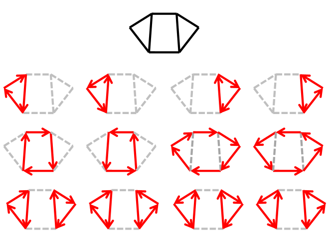
Figure 2: Example of a graph (top) and its respective set of oriented disjoint cycles, consisting of $12$ configurations. Oriented Disjoint cycles are shown in red.

II Determinant as a Series over Monomer-Dimer Contributions

Eqs. (7-10,12) of Chernyak and Chertkov (2008) represent the starting point for discussion of this Section. However, instead of following the path discussed in Chernyak and Chertkov (2008), we make another non-BP choice of the gauge.

The special gauges we will be using are associated with the graph orientations ${\bm{\partial}}\in O({\cal G})$, where $O({\cal G})$ denotes the set of graph orientations. An orientation of ${\cal G}$ associates a direction (“arrow”) on each edge, i.e., it is a pair of maps $\partial_{j}:{\cal G}_{1}\to{\cal G}_{0}$ with $j=0,1$ so that the edge $\alpha$ connects $\partial_{0}(\alpha)$ and $\partial_{1}(\alpha)$. For each edge there are two possible orientations: $\partial_{0}(\{a,b\})=a$, $\partial_{1}(\{a,b\})=b$ and $\partial_{0}(\{a,b\})=b$, $\partial_{1}(\{a,b\})=a$. In particular ${\rm card}(O({\cal G}))=2^{N_{1}({\cal G})}$, where $N_{k}={\rm card}({\cal G}_{k})$ with $k=0,1$ represent the number of edges and nodes. Therefore, orientation can be viewed as a binary variable that resides on the graph edges. The gauge associated with an orientation ${\bm{\partial}}\in O({\cal G})$, which is totally determined by specifying the set $\{\gamma_{ab}({\bm{\partial}})\}_{a\sim b}$ of numbers that characterize the local ground states, is given by

$$\gamma_{ab}({\bm{\partial}}) = (H_{ab})^{-1}\;\;{\rm for}\;a=\partial_{0}(\{a,b\}),\;\;\gamma_{ab}({\bm{\partial}})=-(H_{ab})^{-1}\;\;{\rm for}\;a=\partial_{1}(\{a,b\}),$$

$$\kappa_{ab} = 1,\;\;c_{ab}=1/2,\;\;\gamma^{\prime}_{ab}=-\gamma_{ab},\;\;\;\zeta_{ab}=(H_{ab})^{-1}$$ (16)

which simply means that we choose $\gamma_{ab}=\pm(H_{ab})^{-1}$ depending on orientation, and the signs in front of $H_{ab}$ and $H_{ba}$ are always opposite. The rest of the parameters are determined by Eq. (12) of Chernyak and Chertkov (2008). Note that the set of parameters $\{\gamma_{ab}({\bm{\partial}})\}_{a\sim b}$ for a gauge choice given by Eq. (II) satisfy all the necessary requirements represented by Eq. (11) of Chernyak and Chertkov (2008). Also note that two graph orientations ${\bm{\partial}}$ and ${\bm{\partial}}^{\prime}$ are also related via a set ${\bm{\sigma}}$ of edge binary variables: we define $\sigma_{\{a,b\}}=1$ if $\partial(\{a,b\})=\partial^{\prime}(\{a,b\})$, and $\sigma_{\{a,b\}}=-1$, otherwise. In particular, a choice of some base graph orientation allows the graph orientations to be described using the edge binary variables ${\bm{\sigma}}$. However, a generic unoriented graph is not equipped with a preferred choice of orientation.

For any choice of a special gauge (II) the Grassman integral representation (Eq. (7) of Chernyak and Chertkov (2008)) for the determinant of $H$ can be represented in the following form

$$\det(H)=\left(\prod_{\{a,b\}\in{\cal G}_{1}}(-H_{ab}H_{ba})\right)\left(\prod_{a\in{\cal G}_{0}}H_{aa}\right)\int{\cal D}{\bm{\chi}}{\cal D}\bar{{\bm{\chi}}}\prod_{a\in{\cal G}_{0}}e^{(H_{aa})^{-1}\sum_{b\in{\cal G}_{0}}^{b\sim a}\bar{\chi}_{ba}\sum_{b^{\prime}\in{\cal G}_{0}}^{b^{\prime}\sim a}\chi_{b^{\prime}a}}$$

$$\times\prod_{\{a,b\}\in{\cal G}_{1}}\left(\underbrace{1-\frac{\bar{\chi}_{ab}\chi_{ab}\bar{\chi}_{ba}\chi_{ba}}{H_{ab}H_{ba}}}_{\mbox{even states at }\{a,b\}}+\underbrace{\frac{\bar{\chi}_{ab}\chi_{ba}}{H_{ab}}+\frac{\bar{\chi}_{ba}\chi_{ab}}{H_{ba}}}_{\mbox{odd states at }\{a,b\}}\right),$$ (17)

which is explicitly independent on the choice of a special gauge. We further partition each factor on the second line of Eq. (II) that corresponds to an edge $\{a,b\}$ into a sum of two terms, referred to even and, odd according to the terminology introduced (and explained) in Chernyak and Chertkov (2008). Our next step is to expand the product of edge terms in the integrand of Eq. (II) into a polynomial over the odd states, followed by performing integration over the edge Grassman variables that correspond to the odd contributions. For a given choice of the local odd states we denote by $C\subset{\cal G}$ the subgraph of ${\cal G}$ formed by the edges, where the odd terms [the third or forth term in the second line of Eq. (II)] have been chosen. We start with demonstrating that all vertices of the subgraph $C\subset{\cal G}$ have the valence two, i.e., $C$ is represented by a disjoint union of simple loops. This follows from the fact that the expression in the exponent in Eq. (II) is actually a product of two linear combinations of the original Grassman variables and, therefore

$$e^{(H_{aa})^{-1}\sum_{b\in{\cal G}_{0}}^{b\sim a}\bar{\chi}_{ba}\sum_{b^{\prime}\in{\cal G}_{0}}^{b^{\prime}\sim a}\chi_{b^{\prime}a}}=1+(H_{aa})^{-1}\sum_{b\in{\cal G}_{0}}^{b\sim a}\bar{\chi}_{ba}\sum_{b^{\prime}\in{\cal G}_{0}}^{b^{\prime}\sim a}\chi_{b^{\prime}a}.$$ (18)

Consider a vertex $a\in C_{0}$. For the integral over the local vertex variables $d{\bm{\chi}}_{a}d\bar{\bm{\chi}}_{a}$ not to vanish the integrand should contain each of the local variables $\chi_{ba}$ and $\bar{\chi}_{ba}$ with $b\sim a$ exactly once. These local variables in the integrand originate from the odd terms, described above, from the even terms [second contribution in the second line of Eq. (II)] and from the relevant exponential terms represented by Eq. (18). If an edge $\{b,a\}\in{\cal G}_{1}$ also belongs to $C$ we have either the odd term $(H_{ab})^{-1}\bar{\chi}_{ab}\chi_{ba}$ or $(H_{ba})^{-1}\bar{\chi}_{ba}\chi_{ab}$ in the integrand. Consider the first option (the second option is considered in a similar way), the local conjugate variable $\bar{\chi}_{ba}$ can originate only from the vertex term given by Eq. (18) and is represented by a contribution $(H_{aa})^{-1}\bar{\chi}_{ba}\chi_{b^{\prime}a}$. The variable $\bar{\chi}_{b^{\prime}a}$ conjugate to the the variable $\chi_{b^{\prime}a}$ can originate only from an odd edge contribution, namely $(H_{b^{\prime}a})^{-1}\bar{\chi}_{b^{\prime}a}\chi_{b^{\prime}a}$, which implies that $\{b^{\prime},a\}\in C_{1}$. The edges $\{b,a\}$ and $\{b^{\prime},a\}$ are the only edges adjacent to the node $a$ that belong to $C_{1}$ since the vertex term [Eq. (18)] that provides the conjugate. local variables contains products of only two Grassmans. Consideration of the other odd edge term $(H_{ba})^{-1}\bar{\chi}_{ba}\chi_{ab}$ leads to a similar result, but with the opposite orientation. Therefore, any vertex $a\in C$ has the valence two, and, therefore $C\in\mbox{ODC}({\cal G})$.

Consider a simple oriented loop $(a_{1},\ldots,a_{n})$, where naturally $a_{j}\sim a_{j+1}$ and $a_{n}\sim a_{1}$. The associated contribution given by the integral of the loop edge variables of the product of the edge and vertex contributions has a form $\prod_{j=1}^{n}(H_{a_{j}a_{j}})^{-1}\prod_{j=1}^{n}(H_{a_{j-1}a_{j}})^{-1}I_{a_{1}\ldots a_{n}}$, where

$$I_{a_{1}\ldots a_{n}} = \int\prod_{j=1}^{n}d\chi_{a_{j-1}a_{j}}d\bar{\chi}_{a_{j-1}a_{j}}d\chi_{a_{j+1}a_{j}}d\bar{\chi}_{a_{j+1}a_{j}}\bar{\chi}_{a_{1}a_{2}}\chi_{a_{2}a_{1}}\bar{\chi}_{a_{2}a_{3}}\chi_{a_{3}a_{2}}\bar{\chi}_{a_{3}a_{4}}\chi_{a_{4}a_{3}}\ldots\bar{\chi}_{a_{n}a_{1}}\chi_{a_{1}a_{n}}$$ (19)

$$\times \prod_{j=1}^{n}\bar{\chi}_{a_{j+1}a_{j}}\chi_{a_{j-1}a_{j}}$$

$$= (-1)^{n-1}\prod_{j=1}^{n}\int d\chi_{a_{j-1}a_{j}}d\bar{\chi}_{a_{j-1}a_{j}}d\chi_{a_{j+1}a_{j}}d\bar{\chi}_{a_{j+1}a_{j}}\bar{\chi}_{a_{j-1}a_{j}}\chi_{a_{j+1}a_{j}}\bar{\chi}_{a_{j+1}a_{j}}\chi_{a_{j-1}a_{j}}=-1$$

and in Eq. (19) we use a cyclic convention $j+n=j$. The first equality in Eq. (19) is obtained by performing permutations in the following way. We start with moving the Grassman $\chi_{a_{4}a_{3}}$ in the integrand by two places to the left, followed by moving the combination $\bar{\chi}_{a_{2}a_{3}}\chi_{a_{4}a_{3}}$ to combine it with the combination $\bar{\chi}_{a_{4}a_{3}}\chi_{a_{2}a_{3}}$ in the product over $j$, which corresponds to the value $j=3$; after that we permute the Grassmans $\chi_{a_{3}a_{2}}$ and $\bar{\chi}_{a_{3}a_{4}}$. The overall permutation provides a $(-1)$ sign factor. Repeating a similar operation $(n-1)$ times (including the first explicitly described operation) results in the first equality. The second equality follows from the fact that each of $n$ Grassman integrals in the intermediate expression is equal to $(-1)$.

Due to Eq. (19) the resulting expression for the determinant adopts a form

$$\det(H)=\sum_{C\in\mbox{ODC}({\cal G})}(-1)^{{\rm deg}(C)}\left(\prod_{\{a,b\}\in C}(-H_{ab})\right)Z_{1}({\cal G}\setminus C),$$ (20)

$$Z_{1}({\cal G}\setminus C)=\left(\prod_{\{a,b\}\in({\cal G}_{C})_{1}}(-H_{ab}H_{ba})\right)\left(\prod_{a\in({\cal G}_{C})_{0}}H_{aa}\right)$$

$$\times\int{\cal D}{\bm{\chi}}_{{\cal G}_{C}}{\cal D}\bar{{\bm{\chi}}}_{{\cal G}_{C}}\prod_{a\in{(\cal G}_{C})_{0}}\left(1+(H_{aa})^{-1}\sum_{b\in{(\cal G}_{C})_{0}}^{b\sim a}\bar{\chi}_{ba}\sum_{b^{\prime}\in({\cal G}_{C})_{0}}^{b^{\prime}\sim a}\chi_{b^{\prime}a}\right)\prod_{\{a,b\}\in({\cal G}_{C})_{1}}\left(1-\frac{\bar{\chi}_{ab}\chi_{ab}\bar{\chi}_{ba}\chi_{ba}}{H_{ab}H_{ba}}\right),$$ (21)

where ${\rm deg}(C)$ denotes the number of connected components in $C$. Stated differently, an element $C\in\mbox{ODC}({\cal G})$ is represented by a disjoint union of oriented simple loops with ${\rm deg}(C)$ denoting the number of simple loops in $C$. In Eq. (20) $\bar{{\bm{\chi}}}_{{\cal G}_{C}}$, ${\bm{\chi}}_{{\cal G}_{C}}$ denote the edge Grassman variables restricted to the subgraph ${\cal G}_{C}$, formed by the edges of ${\cal G}$ that do not belong to $C$. In deriving Eq. (21) we have also made use of Eq. (18) to replace the exponential vertex terms with their polynomial counterparts.

It is now straightforward to check [by expanding the integrand in Eq. (21) into a polynomial followed by performing integration over the Grassman variables in Eq. (21)] that $Z_{1}({\cal G}^{\prime})$ is nothing else than the partition function (6) of the monomer-dimer model on the graph ${\cal G}$. Consider an edge $\{a,b\}\in({\cal G}_{C})_{1}$. The Grassman variables $\bar{\chi}_{ab}$, $\bar{\chi}_{ba}$, $\chi_{ab}$ $\chi_{ba}$ whose product provides a nonzero contribution to the integral over the edge variables can originate from the vertex or edge terms in Eq. (21). If they originate from the edge term, then combining with the corresponding edge prefactor [from the first line in Eq. (21)] we obtain the contribution

$$-H_{ab}H_{ba}\int d\chi_{ab}d\bar{\chi}_{ab}d\chi_{ba}d\bar{\chi}_{ba}\left(-\frac{\bar{\chi}_{ab}\chi_{ab}\bar{\chi}_{ba}\chi_{ba}}{H_{ab}H_{ba}}\right)=1,$$ (22)

if they come from the vertex terms associated with the vertices $a$ and $b$, then combined with the corresponding vertex prefactors, the contribution has a form

$$H_{aa}H_{bb}\int d\chi_{ab}d\bar{\chi}_{ab}d\chi_{ba}d\bar{\chi}_{ba}(H_{bb})^{-1}\bar{\chi}_{ab}\chi_{ab}(H_{aa})^{-1}\bar{\chi}_{ba}\chi_{ba}=1.$$ (23)

We call such an edge a dimer. Obviously, any node can have not more than one dimer edge attached to it. The nodes that do not have dimers attached to them are referred to as monomers. A monomer node $a$ does not provide the Grassmans associated with the vertex term and, therefore, the prefactor term $H_{aa}$ is not compensated. A dimer $\{a,b\}$ does not provide the edge terms and, therefore, the edge prefactor $(-H_{ab}H_{ba})$ is not compensated. It is easy to see that any configuration of monomers and dimers that provides a non-zero contribution to the Grassman integral in Eq. (21) satisfies the monomer-dimer matching rules. Therefore, $Z_{1}({\cal G}\setminus C)$ represents the partition function of the monomer-dimer model with the monomer and dimer weights $w_{a}=H_{aa}$ and $w_{ab}=-H_{ab}H_{ba}$, respectively.

Summarizing,

$$\forall C,\quad{\cal G}^{\prime}={\cal G}\setminus C:\quad Z_{1}({\cal G}^{\prime})=Z_{{\rm MD}}({\cal G}^{\prime}).$$ (24)

which implies

$$\det(H)=\sum_{C\in ODC({\cal G})}r(C),\;\;\;r(C)=(-1)^{{\rm deg}(C)}\prod_{(a,b)\in C}(-H_{ab})Z_{{\rm MD}}({\cal G}\setminus C)$$ (25)

To conclude, we just showed that the determinant of a matrix can be represented in terms of a series over disjoint oriented cycles of the underlying graph, with each term of the expansion being proportional to the partition function of the monomer-dimer model defined on the remainder of the graph, i.e., after the cycles, as well as all edges connected to their vertices are removed.

Comparing Eq. (15) with Eq. (25) one finds that in a sense one is an inverse of the other. While the former expresses the partition function of the MD model on the graph in terms of an expansion over the determinants (each corresponds to a directed disjoint cycle), the later does exactly the opposite by expressing the determinant as a series over the partition functions of the MD models each associated with the exclusion of a directed disjoint cycle. More details on this relation are given in Appendix A.

We complete this Section by addressing the issue of the gauge invariance of the simple-loop decomposition. To that end we twist the matrix $H$ as described at the beginning of Section I.1, i.e. introducing the matrix $H({\bm{\sigma}})$, twisted by the gauge field ${\bm{\sigma}}$ as $H_{ab}({\bm{\sigma}})=\sigma_{ab}H_{ab}$ for $a\neq b$ and $H_{aa}({\bm{\sigma}})=H_{aa}$. Applying Eq. (25) to $H({\bm{\sigma}})$, recalling the definition of the $\zeta$-function (1), and noting that the partition functions $Z_{{\rm MD}}({\cal G}\setminus C)$ are obviously invariant with respect to the twisting we obtain the following decomposition for the $\zeta$-function:

$$\zeta({\bm{\sigma}})=\det(H({\bm{\sigma}}))=\sum_{C\in ODC({\cal G})}(-1)^{{\rm deg}(C)}\prod_{(a,b)\in C}(-\sigma_{ab}H_{ab})Z_{{\rm MD}}({\cal G}\setminus C)=\sum_{C\in ODC({\cal G})}r(C)\prod_{(a,b)\in C}\sigma_{ab}$$ (26)

Therefore, $r(C)$ can be viewed as the coefficients in the expansion of the $\zeta$-function $\zeta({\bm{\sigma}})$ in the gauge field ${\bm{\sigma}}$ and, therefore they do not depend on a particular way they are evaluated.

III Summary and Conclusions

To summarize, this manuscript reports new relations between the partition function $Z_{MD}({\cal G})$ of the monomer-dimer model, defined on an arbitrary graph ${\cal G}$ and the corresponding determinant of the matrix $H$ and its minors, constructed from the monomer-dimer weights on the graph. We have formulated a Graphical Gauge Model (GGM) on a graph, stated in terms of Grassman variables and binary gauge fields, so that all the relations reported in the paper follow in a straightforward way via simple and natural manipulations (reparametrizations and integrations) over the partition function of the GGM. Some results of this paper are also linked to the discussions in the first paper of the series Chernyak and Chertkov (2008). In particular, we show here that the expression for a determinant as an expansion over directed disjoint cycles is related to the Loop Series approach of Chernyak and Chertkov (2008). The difference comes from different gauge choices.

In spite of the progress in understanding relations between determinants, loops and matchings (i.e. valid configurations of the monomer-dimer problems), there are still many important challenges left for future analysis. We conclude with mentioning some of these “natural” challenges.

• Given the prominent role the determinants play in the classical studies of the dimer models on planar graphs and graphs embedded in Riemann surfaces of finite genus Kasteleyn (1963); Regge and Zecchina (1996); Galluccio and Loebl (1999a, b); Regge and Zecchina (2000); Cimasoni and Reshetikhin (2007, 2008), one suggests that it should be important to analyze the consequences of the monomer-dimer, determinant, loops and GGM relations discussed above for planar and surface graphs, also extending the results of Chertkov et al. (2008).

• All the Loop Series related constructions for graphical models, introduced so far in Chertkov and Chernyak (2006a, b); Chernyak and Chertkov (2007); Chertkov et al. (2008); Chernyak and Chertkov (2008) and this manuscript, express the partition functions as series over sub-graphs. On the other hand, the well-known formula $\ln\det(H)={\rm Tr}\ln(H)$, and related famous expressions for the log-partition function of the Ising model on a planar graph Kac and Ward (1952), suggests that a multiplicative expansion that represents the partition functions as a product over sub-graphs, may also exist, at least for some class of graphical models. Exploring possible multiplicative decompositions constitutes an important theoretical and algorithmic challenge.

• One general technical conclusion of the paper is related to the use of Berezin integrals Berezin (1987). Our approach shows that the Grassman-integration technique can be useful for deriving quantitative exact relations in graphical statistical problems of computer science, operation research, and information theory. Obviously, the two papers of the series present only the first step in this direction. A possible extension of this approach, worth a future exploration, would be to develop a more general super-symmetrical and $\sigma$-models based approach, in the spirit of Efetov (1997), combining normal and Grassman integrations.

• To a large extent, the practical utility of the determinant and cycle series discussed in the paper is yet to be determined. In particular, it remains to be seen weather the reported cycle series allows an efficient deterministic approximation for the monomer-dimer model partition function. We speculate that an algorithmic extension of our results may lead to the development of novel Fully Polynomial-Time Approximation Schemes (FPTAS) for various hard, $\#P$, weighted counting problems (see e.g. Bayati et al. (2007) for a sample FPTAS example discussed recently).

IV Acknowledgements

We are grateful to J. Johnson for useful comments. This material is based upon work supported by the National Science Foundation under CHE-0808910. The work at LANL was carried out under the auspices of the National Nuclear Security Administration of the U.S. Department of Energy at Los Alamos National Laboratory under Contract No. DE-AC52-06NA25396.

Appendix A Correspondence between Monomer-Dimer model and Determinant Series

In this Appendix we establish relation between Eq. (15) and Eq. (25) in a somehow straightforward way.

A particular strength of the decomposition of the determinant Eq. (25) is its naturality, i.e., it is valid for any graph ${\cal G}$ associated with some matrix $H$. In particular it can be written for any subgraph ${\cal G}^{\prime}\subset{\cal G}$. To see the advantages of naturality in a more clear way we introduce the following notation $X_{C}=\det({\cal G}\setminus C)$ and $Y_{C}=Z_{{\rm MD}}({\cal G}\setminus C)$ where $C\in ODC({\cal G})$ is an (oriented) simple loop in ${\cal G}$. For our purposes it is also convenient to introduce an oriented graph ${\cal C}_{\cdot}({\cal G})$ of simple loops, whose nodes are simple loops $C\in ODC({\cal G})$, i.e., ${\cal C}_{0}({\cal G})=ODC({\cal G})$. The set of links of an oriented graph ${\cal C}_{1}({\cal G})\subset{\cal C}_{0}({\cal G})\times{\cal C}_{0}({\cal G})$ is naturally a subset ${\cal C}_{1}({\cal G})\subset ODC({\cal G})$ and is defined as follows. We say that $(C,C^{\prime})$ is an oriented link (a connecting arrow goes from $C^{\prime}$ to $C$), i.e. $(C,C^{\prime})\in{\cal C}_{1}({\cal G})$, if $C\subset C^{\prime}$.

The reason why the graph ${\cal C}_{\cdot}={\cal C}_{\cdot}({\cal G})$ has been introduced is that ${\cal C}_{\cdot}$ is the oriented graph associated with the linear relation (matrix) that expresses the set $\{X_{C}\}_{C\in{\cal C}_{0}}$ of partition functions in terms of the set $\{Y_{C}\}_{C\in{\cal C}_{0}}$ of partition functions. To see that we recast Eq. (25) for an arbitrary subgraph ${\cal G}^{\prime}\subset{\cal G}$

$$\det({\cal G}^{\prime})=\sum_{C\in ODC({\cal G}^{\prime})}(-1)^{{\rm deg}(C)}\prod_{(a,b)\in C}(-H_{ab})Z_{{\rm MD}}({\cal G}^{\prime}\setminus C).$$ (27)

Applying Eq. (27) for all ${\cal G}^{\prime}={\cal G}\setminus C$ and making use of the introduced notation we arrive at

$$X_{C}=\sum_{C^{\prime}\supset C}R_{CC^{\prime}}Y_{C^{\prime}}=\sum_{C^{\prime}}^{(C,C^{\prime})\in{\cal C}_{1}}R_{CC^{\prime}}Y_{C^{\prime}},\;\;\;R_{CC^{\prime}}=(-1)^{{\rm deg}(C^{\prime}\setminus C)}\prod_{(a,b)\in C^{\prime}\setminus C}(-H_{ab}),\;\;\;R_{CC}=1.$$ (28)

Note that $R_{CC^{\prime}}\neq 0$, if and only if $(C,C^{\prime})\in{\cal C}_{1}$, i.e., $(C,C^{\prime})$ is an edge of the oriented graph ${\cal C}_{\cdot}$, which means that ${\cal C}_{\cdot}$ is the oriented graph associated with the matrix $R_{CC^{\prime}}$.

The oriented disjoint cycle expansion (15) for $Z_{{\rm MD}}$ is obtained by expressing the inverse matrix $R_{CC^{\prime}}^{-1}$ as a sum over the oriented (i.e., orientation on the path should be compatible with the orientation on the graph) paths on the associated graph ${\cal C_{\cdot}}$:

$$Y_{C}=\sum_{C^{\prime}}R_{CC^{\prime}}^{-1}X_{C^{\prime}},\;\;\;R_{CC^{\prime}}^{-1} = \sum_{p\in P{\cal C}_{\cdot}}^{p_{0}=C^{\prime},p_{l(p)}=C}(-1)^{l(p)}\prod_{j=0}^{l(p)-1}R_{p_{j+1}p_{j}}$$ (29)

$$= \prod_{(a,b)\in C^{\prime}\setminus C}(-H_{ab})\sum_{p\in P{\cal C}_{\cdot}}^{p_{0}=C^{\prime},p_{l(p)}=C}(-1)^{l(p)+{\rm deg}(C^{\prime})-{\rm deg}(C)}=\prod_{(a,b)\in C^{\prime}\setminus C}(-H_{ab}).$$

In deriving Eq. (29) we made use of the fact $R_{CC}=1$ for the diagonal elements and the expression for the off-diagonal components (28). In particular the specific form of $R_{CC^{\prime}}$ implies that the contributions of different paths are the same up to a sign. The last equality in Eq. (29) is obtained by an explicit computation of the combinatorial factor

$$\sum_{l=0}^{{\rm deg}(C^{\prime})-{\rm deg}(C)}(-1)^{l(p)+{\rm deg}(C^{\prime})-{\rm deg}(C)}{\cal N}\left(l;{\rm deg}(C^{\prime})-{\rm deg}(C)\right)=1$$ (30)

where ${\cal N}(l;N)$ is the number of ways one can put $N$ objects into $l$ boxes with each box containing at least one object.

Applying Eq. (30) to $C=\emptyset$ and recalling the meaning of the notation $X_{C}$ and $Y_{C}$ we arrive at Eq. (15).

Appendix B Expansion of a Determinant and Summation over the Gauges

In this Appendix we present an alternative derivation of the decomposition (25) of a determinant into a sum over the oriented disjoint cycles with the individual contributions expressed in terms of the partition functions of the Monomer-Dimer (MD) models defined on the proper subgraphs of ${\cal G}$.

First of all we note that the loop decomposition (Eq. (22) of Chernyak and Chertkov (2008)) is valid in any gauge, i.e., for any choice of the set $\{\gamma_{ab}\}_{a\sim b}$, provided that the summation over generalized loops $C\in GL({\cal G})$ is extended to the summation over all subgraphs ${\cal G}^{\prime}\subset{\cal G}$. In the case of a BP gauge the latter summation is restricted to the summation over the generalized loops, since the BP gauge ensures the vanishing of the rest of the contributions. Multiplying the relative contributions $r(C,C^{\prime})$ with the prefactor and changing the order of the summations we recast the loop decomposition in a form

$$\det(H)=\sum_{C\in ODC({\cal G})}r(C),\;\;\;r(C)=\sum_{{\cal G}^{\prime}\subset{\cal G}}^{C\subset{\cal G}^{\prime}}Z({\cal G}^{\prime},C),$$ (31)

of a decomposition in oriented disjoint cycles. Note that in this notation the BP contribution corresponds to the empty simple loop and empty subgraph. Note that strictly speaking the loop series depends on the gauge choice. However, the gauge freedom (among the gauges we are dealing with) belongs to the boson subspace, which implies that the coefficients $r(C)$ in Eq. (31) should be gauge invariant. This issue is addressed at the end of section II.

We will consider the loop series (31) for all $2^{N_{1}}$ special gauges associated with the graph orientations (they are given by Eq. (II)) and average it with an equal weight of $2^{-N_{1}}$. This is a legitimate procedure since the sum of all terms in a loop series is naturally gauge invariant. We also note that for given $C\in ODC({\cal G})$ a particular choice of a subgraph $C\subset{\cal G}^{\prime}\subset{\cal G}$ can be described by a particular configuration of a set ${\bm{\sigma}}\in M_{C}$ of binary variables that reside on those edges of ${\cal G}$ that do not belong to $C$. Namely, $\sigma_{\alpha}=-1$ for $\alpha\in{\cal G}^{\prime}$ (painted edge that correspond to local even excited state) and $\sigma_{\alpha}=1$ otherwise (local ground state). Combining these arguments with the expressions for the ingredients of the loop expansion )Eqs. (23) and (24) in Chernyak and Chertkov (2008)) we arrive at

$$Z = 2^{-N_{1}({\cal G})}\sum_{{\bm{\partial}}\in O({\cal G})}\sum_{C\in ODC({\cal G})}\sum_{{\cal G}^{\prime}\subset{\cal G}}^{C\subset{\cal G}^{\prime}}Z({\cal G}^{\prime},C;{\bm{\partial}})$$ (32)

$$= 2^{-N_{1}({\cal G})}\sum_{C\in ODC({\cal G})}\sum_{{\bm{\partial}}\in O({\cal G})}\sum_{{\bm{\sigma}}\in M_{C}}(-1)^{{\rm deg}(C)}2^{-(N_{1}({\cal G})-N_{1}(C))}\prod_{(c,d)\in C}H_{cd}\prod_{a\in({\cal G}\setminus C)_{0}}\left(-H_{aa}-\sum_{b\sim a}(\gamma_{ba}({\bm{\partial}}))^{-1}\sigma_{ba}\right)$$

$$= 2^{-N_{1}({\cal G})}\sum_{C\in ODC({\cal G})}(-1)^{{\rm deg}(C)}2^{-(N_{1}({\cal G})-N_{1}(C))}$$

$$\times \prod_{(c,d)\in C}H_{cd}\sum_{{\bm{\sigma}}\in M_{C}}\sum_{{\bm{\partial}}\in O({\cal G})}\prod_{a\in({\cal G}\setminus C)_{0}}\left(-H_{aa}-\sum_{b\sim a}(\gamma_{ba}({\bm{\partial}}(\{a,b\})))^{-1}\sigma_{ba}\right).$$

Comparing Eq. (32) with Eqs. (31) we see that the decomposition in simple loops (25) is reproduced if we define

$$Z_{{\rm MD}}({\cal G}\setminus C)=2^{-(N_{1}({\cal G})-N_{1}(C))}\sum_{{\bm{\sigma}}\in M_{C}}2^{-N_{1}({\cal G})}\sum_{{\bm{\partial}}\in O({\cal G})}\prod_{a\in({\cal G}\setminus C)_{0}}\left(-H_{aa}-\sum_{b\sim a}(\gamma_{ba}({\bm{\partial}}(\{a,b\})))^{-1}\sigma_{ba}\right).$$ (33)

The only thing we need to show at this point is that the expression in Eq. (33) reproduces the partition function of the MD model on the graph ${\cal G}\setminus C$. This is achieved by performing the summation over the binary variables ${\bm{\partial}}\in O({\cal G})$. The desired result follows from an obvious property

$$\frac{1}{2}\sum_{{\bm{\partial}}(\{a,b\})}\left(\gamma_{ba}({\bm{\partial}}(\{a,b\}))\right)^{-1}\sigma_{ba}=0,\;\;\;\frac{1}{2}\sum_{{\bm{\partial}}(\{a,b\})}\left(\gamma_{ba}({\bm{\partial}}(\{a,b\}))\right)^{-1}\left(\gamma_{ab}({\bm{\partial}}(\{a,b\}))\right)^{-1}\sigma_{ba}\sigma_{ab}=-H_{ab}H_{ba},$$ (34)

where both sums in Eq. (34) contain two terms that correspond to two possible values of the orientation ${\bm{\partial}}(\{a,b\})$ of the edge $\{a,b\}$. A choice of a diagonal term in the parenthesis in Eq. (33) corresponds to having a monomer on the node $a$ with the weight $H_{aa}$. It follows from Eq. (34) that the off-diagonal terms should always go in pairs, each pair $(\gamma_{ab}\gamma_{ba})^{-1}$ corresponds to having a dimer on the link $\{a,b\}$, whose weight is $-H_{ab}H_{ba}$. It also follows from Eq. (34) that the sum over orientations in Eq. (33) does not depend on ${\bm{\sigma}}$ and, therefore, the sum over ${\bm{\sigma}}$ just cancels out the first prefactor in Eq. (33). This completes the proof.

References

- Polyakov (1987) A. M. Polyakov, Gauge fields and strings (Contemporary concepts in physics, Chur, Switzerland: Harwood Academic Publishers, 1987).
- Zinn-Justin (1989) J. Zinn-Justin, Quantum Field Theory and Critical Phenomena, vol. 77 of International Series of Monographs on Physics (Clarendon Press; Oxford University Press, Oxford, U.K.; New York, U.S.A., 1989), 3rd ed.
- Wilson and Kogut (1974) K. G. Wilson and J. Kogut, Physics Reports 12, 75 (1974).
- Chertkov and Chernyak (2006a) M. Chertkov and V. Chernyak, Physical Review E (Statistical, Nonlinear, and Soft Matter Physics) 73, 065102 (pages 4) (2006a), URL http://link.aps.org/abstract/PRE/v73/e065102.
- Chertkov and Chernyak (2006b) M. Chertkov and V. Y. Chernyak, Journal of Statistical Mechanics: Theory and Experiment 2006, P06009 (2006b), URL http://stacks.iop.org/1742-5468/2006/P06009.
- Chernyak and Chertkov (2008) V. Y. Chernyak and M. Chertkov, Fermions and loops on graphs. i. loop calculus for determinant (2008).
- Ihara (1966) Y. Ihara, J. Math. Soc. Japan 18, 219 (1966).
- L.Lovász and Plummer (1986) L.Lovász and M. Plummer, Matching Theory (Academic Press, 1986).
- Jerrum (1990) M. Jerrum, Journal of Statistical Physics 59, 1087 (1990).
- Milgram and Penner (1993) R. Milgram and R. Penner, Contemporary Mathematics 150, 247 (1993).
- Spanier (1989) E. Spanier, Algebraic Topology (Springer, 1989).
- Berezin (1987) F. Berezin, Introduction to superanalysis (Reidel Publishing Company, Dordrecht, 1987).
- Kasteleyn (1963) P. W. Kasteleyn, Journal of Mathematical Physics 4, 287 (1963), URL http://link.aip.org/link/?JMP/4/287/1.
- Regge and Zecchina (1996) T. Regge and R. Zecchina, Journal of Mathematical Physics 37, 2796 (1996).
- Galluccio and Loebl (1999a) A. Galluccio and M. Loebl, Electronic Journal of Combinatorics, 6(1). Research Paper 6 p. 18 (1999a).
- Galluccio and Loebl (1999b) A. Galluccio and M. Loebl, Electronic Journal of Combinatorics, 6(1). Research Paper 7 p. 7 (1999b).
- Regge and Zecchina (2000) T. Regge and R. Zecchina, Journal of Physics A Mathematical General 33, 741 (2000).
- Cimasoni and Reshetikhin (2007) D. Cimasoni and N. Reshetikhin, Communications in Mathematical Physics 275, 187 (2007), URL http://www.springerlink.com/content/a2m2385607g31614.
- Cimasoni and Reshetikhin (2008) D. Cimasoni and N. Reshetikhin, Communications in Mathematical Physics 281, 445 (2008), URL http://www.springerlink.com/content/74454243n7281kv6.
- Chertkov et al. (2008) M. Chertkov, V. Y. Chernyak, and R. Teodorescu, Journal of Statistical Mechanics: Theory and Experiment 2008, P05003 (19pp) (2008), URL http://stacks.iop.org/1742-5468/2008/P05003.
- Chernyak and Chertkov (2007) V. Y. Chernyak and M. Chertkov, Information Theory, 2007. ISIT 2007. IEEE International Symposium on pp. 316–320 (2007), URL http://arxiv.org/abs/cs.IT/0701086.
- Kac and Ward (1952) M. Kac and J. Ward, Physical Review 88 (1952).
- Efetov (1997) K. Efetov, Sypersimmetry in Disorder and Chaos (Cambridge University Press, 1997).
- Bayati et al. (2007) M. Bayati, D. Gamarnik, D. Katz, C. Nair, and P. Tetali, in STOC ’07: Proceedings of the thirty-ninth annual ACM symposium on Theory of computing (ACM, New York, NY, USA, 2007), pp. 122–127.