Effect of Slow Switching in On-line Learning for Ensemble Teachers

Abstract

We have analyzed the generalization performance of a student which slowly switches ensemble teachers. By calculating the generalization error analytically using statistical mechanics in the framework of on-line learning, we show that the dynamical behaviors of generalization error have the periodicity that is synchronized with the switching period and the behaviors differ with the number of ensemble teachers. Furthermore, we show that the smaller the switching period is, the larger the difference is.

Learning can be classified into batch learning and on-line learning [1, 2]. In on-line learning, examples once used are discarded and a student cannot give correct answers for all examples used in training. However, there are merits; for example, a large memory for storing many examples is not necessary and it is possible to follow a time variant teacher[3, 4]. Recently, we used a statistical mechanical method[1, 5] to analyze the generalization performance of a model composed of linear perceptrons: a true teacher, ensemble teachers, and the student in the framework of on-line learning[6]. That is, we treated a model that has $K$ teachers called ensemble teachers who exist around a true teacher[7]. In the study, we analyzed the model in which a student switches the ensemble teachers in turn or randomly at each time step. Therefore, the study was an analysis of a fast switching model. On the contrary, the properties of a model in which a student switches the ensemble teachers slowly is also attractive. In this letter, we analyze such a slow switching model.

We have considered a true teacher, $K$ ensemble teachers, and a student. They are all linear perceptrons with connection weights $A$, $\mbox{\boldmath$B$}_{k}$, and $J$, respectively. Here, $k=1,\ldots,K$. For simplicity, the connection weight of the true teacher, the ensemble teachers, and the student is simply called the true teacher, the ensemble teachers, and the student, respectively. The true teacher $\mbox{\boldmath$A$}=\left(A_{1},\ldots,A_{N}\right)$, ensemble teachers $\mbox{\boldmath$B$}_{k}=\left(B_{k1},\ldots,B_{kN}\right)$, student $\mbox{\boldmath$J$}=\left(J_{1},\ldots,J_{N}\right)$, and input $\mbox{\boldmath$x$}=\left(x_{1},\ldots,x_{N}\right)$ are $N$-dimensional vectors. Each component $A_{i}$ of $A$ is drawn from ${\cal N}(0,1)$ independently and fixed, where ${\cal N}(0,1)$ denotes the Gaussian distribution with a mean of zero and a variance of unity. Some components $B_{ki}$ are equal to $A_{i}$ multiplied by –1, the others are equal to $A_{i}$. Which component $B_{ki}$ is equal to $-A_{i}$ is independent from the value of $A_{i}$. Hence, $B_{ki}$ also obeys ${\cal N}(0,1)$ and it is also fixed. The direction cosine between $\mbox{\boldmath$B$}_{k}$ and $A$ is $R_{Bk}$ and that between $\mbox{\boldmath$B$}_{k}$ and $\mbox{\boldmath$B$}_{k^{\prime}}$ is $q_{kk^{\prime}}$. Each of the components $J_{i}^{0}$ of the initial value $\mbox{\boldmath$J$}^{0}$ of $J$ is drawn from ${\cal N}(0,1)$ independently. The direction cosine between $J$ and $A$ is $R_{J}$ and that between $J$ and $\mbox{\boldmath$B$}_{k}$ is $R_{BkJ}$. Each component $x_{i}$ of $x$ is drawn from ${\cal N}(0,1/N)$ independently.

This letter assumes the thermodynamic limit $N\rightarrow\infty$. Therefore, $\|\mbox{\boldmath$A$}\|=\|\mbox{\boldmath$B$}_{k}\|=\|\mbox{\boldmath$J$}^{0}\|=\sqrt{N}$, and $\|\mbox{\boldmath$x$}\|=1$. Generally, norm $\|\mbox{\boldmath$J$}\|$ of the student changes as time step proceeds. Therefore, ratio $l^{m}$ of the norm to $\sqrt{N}$ is introduced and called the length of the student. That is, $\|\mbox{\boldmath$J$}^{m}\|=l^{m}\sqrt{N}$, where $m$ denotes the time step. The outputs of the true teacher, the ensemble teachers, and the student are $y^{m}+n_{A}^{m}$, $v_{k}^{m}+n_{Bk}^{m}$ and $u^{m}l^{m}+n_{J}^{m}$, respectively. Here, $y^{m}=\mbox{\boldmath$A$}\cdot\mbox{\boldmath$x$}^{m}$, $v_{k}^{m}=\mbox{\boldmath$B$}_{k}\cdot\mbox{\boldmath$x$}^{m}$, and $u^{m}l^{m}=\mbox{\boldmath$J$}^{m}\cdot\mbox{\boldmath$x$}^{m}$ where $y^{m}$, $v_{k}^{m}$, and $u^{m}$ obey Gaussian distributions with a mean of zero and a variance of unity. $n_{A}^{m}$, $n_{Bk}^{m}$, and $n_{J}^{m}$ are independent Gaussian noises with variances of $\sigma_{A}^{2},\sigma_{Bk}^{2}$, and $\sigma_{J}^{2}$, respectively.

We define the error $\epsilon_{Bk}$ between true teacher $A$ and each member $\mbox{\boldmath$B$}_{k}$ of the ensemble teachers by the squared errors of their outputs: $\epsilon_{Bk}^{m}\equiv\frac{1}{2}\left(y^{m}+n_{A}^{m}-v_{k}^{m}-n_{Bk}^{m}\right)^{2}$. In the same manner, we define error $\epsilon_{BkJ}$ between each member $\mbox{\boldmath$B$}_{k}$ of the ensemble teachers and student $J$ by the squared errors of their outputs: $\epsilon_{BkJ}^{m}\equiv\frac{1}{2}\left(v_{k}^{m}+n_{Bk}^{m}-u^{m}l^{m}-n_{J}^{m}\right)^{2}$. Student $J$ adopts the gradient method as a learning rule and uses input $x$ and an output of one of the $K$ ensemble teachers $\mbox{\boldmath$B$}_{k}$. Here, the student $J$ uses each ensemble teacher $\mbox{\boldmath$B$}_{k}$ $TN$ times succsessively where $T$ is $O(1)$. That is,

$$\mbox{\boldmath$J$}^{m+1} = \mbox{\boldmath$J$}^{m}-\eta\frac{\partial\epsilon_{BkJ}^{m}}{\partial\mbox{\boldmath$J$}^{m}}$$ (1)

$$= \mbox{\boldmath$J$}^{m}+\eta\left(v_{k}^{m}+n_{Bk}^{m}-u^{m}l^{m}-n_{J}^{m}\right)\mbox{\boldmath$x$}^{m},$$ (2)

$$k = \mbox{mod}\left(\left[\frac{m}{TN}\right],K\right)+1,$$ (3)

where $\eta$ denotes the learning rate and is a constant number. The Gauss notation is denoted by $\left[\cdot\right]$. That is, $\left[\frac{m}{TN}\right]$ is the maximum integer which is not larger than $\frac{m}{TN}$. Here, $\mbox{mod}\left(\left[\frac{m}{TN}\right],K\right)$ denotes the remainder of $\left[\frac{m}{TN}\right]$ divided by $K$. Equation (3) means that the student uses each ensemble teacher $TN\sim O(N)$ times succsessively. We call this slow switching. By generalizing the learning rules, Eq. (2) can be expressed as $\mbox{\boldmath$J$}^{m+1}=\mbox{\boldmath$J$}^{m}+f_{k}\mbox{\boldmath$x$}^{m}$, where $f$ denotes a function that represents the update amount and is determined by the learning rule. In addition, we define the error $\epsilon_{J}$ between true teacher $A$ and student $J$ by the squared error of their outputs: $\epsilon_{J}^{m}\equiv\frac{1}{2}\left(y^{m}+n_{A}^{m}-u^{m}l^{m}-n_{J}^{m}\right)^{2}$.

One of the goals of statistical learning theory is to theoretically obtain generalization errors. Since generalization error is the mean of errors for the true teacher over the distribution of new input and noises, generalization error $\epsilon_{Bkg}$ of each member $\mbox{\boldmath$B$}_{k}$ of the ensemble teachers and $\epsilon_{Jg}$ of student $J$ are calculated as follows. Superscripts $m$, which represent the time step, are omitted for simplicity unless stated otherwise.

$$\epsilon_{Bkg} = \int d\mbox{\boldmath$x$}dn_{A}dn_{Bk}P\left(\mbox{\boldmath$x$},n_{A},n_{Bk}\right)\epsilon_{Bk}$$ (4)

$$= \int dydv_{k}dn_{A}dn_{Bk}P\left(y,v_{k},n_{A},n_{Bk}\right)\frac{1}{2}\left(y+n_{A}-v_{k}-n_{Bk}\right)^{2}$$ (5)

$$= \frac{1}{2}\left(-2R_{Bk}+2+\sigma_{A}^{2}+\sigma_{Bk}^{2}\right),$$ (6)

$$\epsilon_{Jg} = \int d\mbox{\boldmath$x$}dn_{A}dn_{J}P\left(\mbox{\boldmath$x$},n_{A},n_{J}\right)\epsilon_{J}$$ (7)

$$= \int dydudn_{A}dn_{J}P\left(y,u,n_{A},n_{J}\right)\frac{1}{2}\left(y+n_{A}-ul-n_{J}\right)^{2}$$ (8)

$$= \frac{1}{2}\left(-2lR_{J}+l^{2}+1+\sigma_{A}^{2}+\sigma_{J}^{2}\right).$$ (9)

To simplify the analysis, two auxiliary order parameters $r_{J}\equiv lR_{J}$ and $r_{BkJ}\equiv lR_{BkJ}$ are introduced. Simultaneous differential equations in deterministic forms [5], which describe the dynamical behaviors of order parameters when the student uses a teacher $\mbox{\boldmath$B$}_{k^{\prime}}$ that consists of ensemble teachers have been obtained on the basis of self-averaging in the thermodynamic limits as follows:

$$\frac{dr_{BkJ}}{dt} =\langle f_{k^{\prime}}v_{k}\rangle, \frac{dr_{J}}{dt} =\langle f_{k^{\prime}}y\rangle, \frac{dl}{dt} =\langle f_{k^{\prime}}u\rangle+\frac{1}{2l}\langle f_{k^{\prime}}^{2}\rangle.$$ (10)

Here, dimension $N$ has been treated to be sufficiently greater than the number $K$ of ensemble teachers. Time is defined by $t=m/N$, that is, time step $m$ normalized by dimension $N$. Since linear perceptrons are treated in this letter, the sample averages that appeared in the above equations can be easily calculated as follows:

$$\langle f_{k^{\prime}}u\rangle =\eta\left(\frac{r_{Bk^{\prime}J}}{l}-l\right), \langle f_{k^{\prime}}^{2}\rangle =\eta^{2}\left(l^{2}-2r_{Bk^{\prime}J}+1+\sigma_{Bk^{\prime}}^{2}+\sigma_{J}^{2}\right),$$ (11)

$$\langle f_{k^{\prime}}y\rangle =\eta\left(R_{Bk^{\prime}}-r_{J}\right), \langle f_{k^{\prime}}v_{k}\rangle =\eta\left(q_{k^{\prime}k}-r_{BkJ}\right).$$ (12)

Let us denote the values of $r_{J},r_{BkJ}$, and $l^{2}$ of $t=t_{0}$ as $r_{J}^{t_{0}},r_{BkJ}^{t_{0}}$, and $(l^{2})^{t_{0}}$, respectively. By using these as intitial values, simultaneous differential equations Eqs.(10)–(12) can be solved analytically as follows:

$$r_{BkJ} = q_{k^{\prime}k}+\left(r_{BkJ}^{t_{0}}-q_{k^{\prime}k}\right)e^{-\eta(t-t_{0})},$$ (13)

$$r_{J} = R_{Bk^{\prime}}+\left(r_{J}^{t_{0}}-R_{Bk^{\prime}}\right)e^{-\eta(t-t_{0})},$$ (14)

$$l^{2} = 1+\frac{\eta}{2-\eta}\left(\sigma_{Bk^{\prime}}^{2}+\sigma_{J}^{2}\right)+2\left(r_{Bk^{\prime}J}^{t_{0}}-1\right)e^{-\eta(t-t_{0})}$$ (15)

$$+\left((l^{2})^{t_{0}}-1-\frac{\eta}{2-\eta}\left(\sigma_{Bk^{\prime}}^{2}+\sigma_{J}^{2}\right)-2\left(r_{Bk^{\prime}J}^{t_{0}}-1\right)\right)e^{\eta(\eta-2)(t-t_{0})}.$$

Since all components $A_{i}$ and $J_{i}^{0}$ of true teacher $A$ and the initial student $\mbox{\boldmath$J$}^{0}$ are drawn from ${\cal N}(0,1)$ independently, and because the thermodynamic limit $N\rightarrow\infty$ is also assumed, they are orthogonal to each other at $t=0$. That is, $R_{J}=0$ and $l=1$ when $t=0$.

In the following, we consider the case where direction cosines $R_{Bk}$ between the ensemble teachers and the true teacher, direction cosines $q_{kk^{\prime}}$ among the ensemble teachers and variances $\sigma_{Bk}^{2}$ of the noises of ensemble teachers are uniform. That is,

$$R_{Bk}=R_{B},(k=1,\ldots,K),\ \ \ \ q_{kk^{\prime}}=\left\{\begin{array}[]{ll}1,&(k=k^{\prime}),\\ q,&(\text{otherwise}),\end{array}\right.\ \ \ \ \sigma_{Bk}^{2}=\sigma_{B}^{2}.$$ (16)

The dynamical behaviors of generalization errors $\epsilon_{Jg}$ have been analytically obtained by substituting Eqs. (14) and (15) into Eq. (9). The analytical results and the corresponding simulation results, where $N=10^{5}$ are shown in Figs. 1 and 2. In computer simulations, $\epsilon_{Jg}$ was obtained by averaging the squared errors for $5\times 10^{4}$ random inputs at each time step. In these figures, the curves represent theoretical results. The symbols represent simulation results. In these figures, $R_{B}=0.7$ and $q=0.49$ are common conditions. In addition, $\eta=0.3,\sigma_{A}^{2}=0.1,\sigma_{B}^{2}=0.2$, and $\sigma_{J}^{2}=0.3$ are conditions for Fig. 1. $\eta=1.5,\sigma_{A}^{2}=0.01,\sigma_{B}^{2}=0.02$, and $\sigma_{J}^{2}=0.03$ are conditions for Fig. 2.

Figure 1: Dynamical behaviors of generalization errors $\epsilon_{Jg}$ when $\eta=0.3$. Theory and computer simulations. $R_{B}=0.7,q=0.49,\sigma_{A}^{2}=0.1,\sigma_{B}^{2}=0.2$, and $\sigma_{J}^{2}=0.3$. (a)$T=5.0$, (b)$T=2.0$.

These figures show that the dynamical behaviors of generalization error have the periodicity that is synchronized with the switching period $T$. In the case of $K=2$, the student uses ensemble teachers as $\mbox{\boldmath$B$}_{1}\rightarrow\mbox{\boldmath$B$}_{2}\rightarrow\mbox{\boldmath$B$}_{1}\rightarrow\mbox{\boldmath$B$}_{2}\rightarrow\cdots$ . In the case of $K=5$, $\mbox{\boldmath$B$}_{1}\rightarrow\mbox{\boldmath$B$}_{2}\rightarrow\mbox{\boldmath$B$}_{3}\rightarrow\mbox{\boldmath$B$}_{4}\rightarrow\mbox{\boldmath$B$}_{5}\rightarrow\mbox{\boldmath$B$}_{1}\rightarrow\mbox{\boldmath$B$}_{2}\rightarrow\mbox{\boldmath$B$}_{3}\rightarrow\cdots$. Therefore, by comparing the behaviors of $K=2$ and that of $K=5$, the generarization errors $\epsilon_{Jg}$ completely agree during the time corresponding to two cycles from the initial state because the teachers used by student are the same. On the contrary, the generarization errors $\epsilon_{Jg}$ of $K=2$ and $K=5$ are not the same after the second cycle. In our study on the fast switching model[6], it was proven that when a student’s learning rate satisfies $\eta<1$, the larger the number $K$ is, the smaller the student’s generalization error is. The same phenomenon is observed in the slow switching model treatd in this letter, that is, the generalization error of $K=5$ is smaller than that of $K=2$ as shown in Fig. 1. On the contrary, the generalization error of $K=5$ is larger than that of $K=2$ in Fig. 2. Here, the dynamical behavior approaches that of the fast switching model[6] asymptotically in the limit of switching period $T\rightarrow 0$.

Figure 2: Dynamical behaviors of generalization errors $\epsilon_{Jg}$ when $\eta=1.5$. Theory and computer simulations. $R_{B}=0.7,q=0.49,\sigma_{A}^{2}=0.01,\sigma_{B}^{2}=0.02$, and $\sigma_{J}^{2}=0.03$. (a)$T=1.0$, (b)$T=0.5$.

In both cases of $\eta=0.3$ and $1.5$, the smaller the switching period $T$ is, the larger the difference between the generalization error $\epsilon_{Jg}$ of $K=2$ and that of $K=5$ is. The reason is the following: if the switching period $T$ is large, a student learns enough from only the one teacher that the student uses in the period. In other words, as the student forgets the other teachers, the influence of the number $K$ of ensemble teachers becomes small.

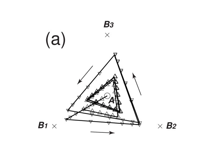
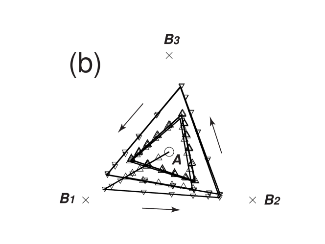
Figure 3: Student’s projection to 2-D plane on which $\mbox{\boldmath$B$}_{1}$–$\mbox{\boldmath$B$}_{3}$ exist. (a)$\eta=0.3$, (b)$\eta=1.5$. Solid lines represent trajectories of student’s projection obtained theoretically. Symbols $\bigtriangleup$ and $\bigtriangledown$ represent computer simulations with (a)$T=2.0$ and $T=5.0$, (b)$T=0.5$ and $T=1.0$, respectively.

We visualize the student’s behaviors in the case of $K=3$ to understand them intuitively. That means we obtain the student’s projection to the two-dimensional plane on which the three ensemble teachers exist. Figure 3 shows the projection’s trajectories in the case of $\eta=0.3$ and $\eta=1.5$. In this figure, symbols $\times$, $\circ$ and solid lines represent the ensemble teachers $\mbox{\boldmath$B$}_{1}$, $\mbox{\boldmath$B$}_{2}$ and $\mbox{\boldmath$B$}_{3}$, the projection of the true teacher $A$ and the trajectories of the student’s projection obtained theoretically, respectively. In Fig. 3(a), symbols $\bigtriangleup$ and $\bigtriangledown$ represent the student’s projections obtained by computer simulations with $T=2.0$ and $T=5.0$, respectively. In Fig. 3(b), those represent the projections with $T=0.5$ and $T=1.0$, respectively. This figure shows that the student moves straight toward the teacher that the student uses then. Therefore, the student’s trajectories in the steady state are regular triangles. The triangles are small when the switching period $T$ is small and the triangles are large when $T$ is large. In this figure, a side of the trajectory corresponds to a period in Figs. 1 and 2. Note that the distance between the student and the true teacher in Fig. 3 is not necessarily related to the real distance between the student and the true teacher nor the generalization error since this figure shows the projections. Though the student is near the true teacher when $T$ is small in Fig. 3(b), the generalization error is small when $T$ is large as shown in Fig. 2.

Figure 4: Means of steady state generalization errors $\epsilon_{Jg}$. Theory. $q=0.49,R_{B}=0.7$ and $\sigma_{A}^{2}=\sigma_{B}^{2}=\sigma_{J}^{2}=0.0$. (a)$T=0.5$, (b)$T=5.0$.

The relationships between the learning rate $\eta$ and the means of steady state generalization errors $\epsilon_{Jg}$ are shown in Fig. 4. The means are measured by averaging the generalization errors during a cycle after the dynamical behaviors reach the steady state. In this figure, when a learning rate satisfies $\eta<1$, the larger the number $K$ is, the smaller the generalization error is. This is the same property with that of the fast switching model[6]. A comparison of Figs. 4(a) and 4(b) shows that the smaller the switching period $T$ is, the larger the difference among the means of generalization errors $\epsilon_{Jg}$ of various $K$ values in the slow switching model as treated in this letter.

Figure 5: Means of steady state generalization errors $\epsilon_{Jg}$. Theory. $K=5,R_{B}=0.7$ and $\sigma_{A}^{2}=\sigma_{B}^{2}=\sigma_{J}^{2}=0.0$. (a)$T=0.5$, (b)$T=5.0$.

The relationships between the learning rate $\eta$ and the means of steady state generalization errors $\epsilon_{Jg}$ for various direction cosines $q$ are shown in Fig. 5. As shown in this figure, when a learning rate satisfies $\eta<1$, the smaller $q$ is, the smaller the generalization error is. This is also the same property as that of the fast switching model[6]. By comparing Figs. 5(a) and 5(b), we see that the smaller the switching period $T$ is, the larger the difference among the means of generalization errors $\epsilon_{Jg}$ of various $q$.

In summary, we have analyzed the generalization performance of a student in a model composed of linear perceptrons: a true teacher, ensemble teachers, and the student. In particular, the case where the student slowly switches ensemble teachers has been analyzed. By calculating the generalization error analytically using statistical mechanics in the framework of on-line learning, we have shown that the dynamical behaviors of generalization error have the periodicity that is synchronized with the switching period and that the behaviors differ with the number of ensemble teachers. Furthermore, we have shown that the smaller the switching period is, the larger the difference is.

References

• [1] D. Saad, (ed.): On-line Learning in Neural Networks (Cambridge University Press, Cambridge, 1998).
• [2] N. Cesa-Bianchi and G. Lugosi: Prediction, Learning, and Games (Cambridge University Press, New York, 2006).
• [3] S. Miyoshi and M. Okada: J. Phys. Soc. Jpn. 75 (2005) 024003.
• [4] M. Urakami, S. Miyoshi, and M. Okada: J. Phys. Soc. Jpn. 76 (2005) 044003.
• [5] H. Nishimori: Statistical Physics of Spin Glasses and Information Processing: An Introduction (Oxford University Press, Oxford, 2001).
• [6] S. Miyoshi and M. Okada: J. Phys. Soc. Jpn. 75 (2006) 044002.
• [7] T. Hirama and K. Hukushima: J. Phys. Soc. Jpn. 77 (2008) 094801.