Reaction Brownian Dynamics and the effect of spatial fluctuations on the gain of a push-pull network

Abstract

Brownian Dynamics algorithms are widely used for simulating soft-matter and biochemical systems. In recent times, their application has been extended to the simulation of coarse-grained models of cellular networks in simple organisms. In these models, components move by diffusion, and can react with one another upon contact. However, when reactions are incorporated into a Brownian Dynamics algorithm, attention must be paid to avoid violations of the detailed-balance rule, and therefore introducing systematic errors in the simulation. We present a Brownian Dynamics algorithm for reaction-diffusion systems that rigorously obeys detailed balance for equilibrium reactions. By comparing the simulation results to exact analytical results for a bimolecular reaction, we show that the algorithm correctly reproduces both equilibrium and dynamical quantities. We apply our scheme to a “push-pull” network in which two antagonistic enzymes covalently modify a substrate. Our results highlight that the diffusive behaviour of the reacting species can reduce the gain of the response curve of this network.

I Introduction

Most, if not all, biological processes are regulated by biomolecules, such as proteins and DNA, which chemically and physically interact with one another in what are called biochemical networks. These networks are often highly non-linear, which means that mathematical modelling is critical for understanding and predicting their behaviour. The dominant paradigm has been to consider the living cell to be a spatially homogeneous environment, analogous to a well-stirred reactor. It is increasingly recognised, however, that the cell is a highly inhomogeneous environment, in which compartmentalisation, scaffolding and localised interactions are actively exploited to enhance the regulatory function of biochemical networks. This means that it becomes important to not only describe the biochemical network in time, but also in space.

In this manuscript, we present an algorithm for simulating biochemical networks in time and space that is based upon Brownian Dynamics. Brownian Dynamics is a stochastic dynamics scheme, in which the solvent is treated implicitly; only solutes are described explicitly. The forces experienced by the solutes contain a contribution from the interactions with the other solutes and a random part, which is the dynamical remnant of the collisions with the solvent molecules. A pioneering BD algorithm was introduced by Ermak and McCammon Ermak and McCammon (1978), and detailed, atomistic Brownian Dynamics simulations have been performed to study the dynamics of enzyme-substrate and protein-protein association reactions Northrup and Erickson (1992); Wade (1996); Huber and Kim (1996); Gabdoulline and Wade (1997); Zou et al. (2000); Gabdoulline and Wade (2001, 2002). More recently, Brownian Dynamics has not only been used to study the association between two proteins, but also to simulate networks of interacting biomolecules Schaff et al. (1997); Andrews and Bray (2004); Stiles (2000). In order to simulate these large systems at the biologically relevant length and time scales, molecules are coarse-grained to the level of simple geometrical objects, which can diffuse and react with other chemical species in a confined geometry.

While Brownian Dynamics algorithms for simulating biochemical networks are based upon a simplified description of the molecules and their interactions, they do go beyond the conventional kinetic Monte Carlo schemes to simulate biochemical networks Gillespie (1977). These algorithms are based upon the zero-dimensional chemical master equation, and, as such, they take into account the discrete nature of the components and the stochastic character of their interactions. However, they assume that at each instant in time the particles are uniformly distributed in space. In contrast, Brownian Dynamics based algorithms take into account not only the particulate nature of the molecules and the probabilistic character of their interactions, but also that at any moment in time the particles may be non-uniformly distributed in space. Brownian Dynamics thus accounts for both temporal and spatial fluctuations of the components. Moreover, it allows for spatial gradients and for localised interactions in the network.

Recently, a number of stochastic techniques have been developed that make it possible to simulate biochemical networks in time and space. Some techniques are based upon Brownian Dynamics Schaff et al. (1997); Andrews and Bray (2004); Stiles (2000), while others are based upon the reaction-diffusion master equation Hattne et al. (2005); Ander et al. (2004); Lemerle et al. (2005); Rodriguez et al. (2006). The advantage of Brownian Dynamics based techniques is that they are truly particle-based, which means that they do not have to rely on a mesoscopic length and time scale on which the system is well-stirred. We have recently developed an entirely novel algorithm, called Green’s Function Reaction Dynamics (GFRD), which is particle-based scheme to simulate biological networks in time and space, like Brownian Dynamics. However, in contrast to Brownian Dynamics, GFRD is an event-driven algorithm, which uses Green’s functions to concatenate the propagation of the particles in space with the chemical reactions between them. This makes GFRD orders of magnitude more efficient than Brownian Dynamics when the concentrations are below $0.1\,-\,1\mu{\rm M}$. For higher concentrations, or for reactions near surfaces, brute-force Brownian Dynamics is more efficient, because of the smaller computational overhead per time step.

Although the main idea of applying Brownian Dynamics to reaction-diffusion systems is straightforward, a number of ingredients has to be examined with care. One is: to which processes do the association and dissociation rates as used in the simulations correspond to? To the intrinsic rates, which are the reaction rates at contact, or to the effective rates that also take into account the effect of diffusion? The other issue is detailed balance. Biochemical networks often contain reactions that do not consume energy or are otherwise driven out of equilibrium. These equilibrium reactions should obey detailed balance. Even though a number of Brownian Dynamics based algorithms have been presented Schaff et al. (1997); Andrews and Bray (2004); Stiles (2000), this question has, to our knowledge, not been systematically addressed.

In this paper, we present a Brownian Dynamics algorithm that rigorously obeys detailed balance and is thus able to reproduce the equilibrium properties of a reaction-diffusion system. In Section II, we derive our algorithm on the basis of the statistical mechanics of chemical reactions. The algorithm is subjected to stringent tests in Section III: besides equilibrium properties, we test also how well the algorithm reproduces the dynamical behavior of a bimolecular reaction, for different values of the time step $\Delta t$. A comparison with a stochastic algorithm that does not account for spatial fluctuations is also presented. Finally, in Section IV we show an illustrative application of our algorithm to a simple coarse-grained model of a chemical species under the action of two enzymes operating in opposite directions (the so-called “push-pull” model system). Simulations conducted with our BD algorithm show that both spatial and temporal fluctuations reduce the gain of the response of the system.

II Methods

II.1 Detailed balance

Before we present the outline of the algorithm in the next section, we discuss the detailed-balance rule that must be obeyed for equilibrium reactions. To this end, we will consider the elementary bimolecular reaction:

$$A+B\rightleftharpoons C\qquad(k_{\rm on},k_{\rm off}).$$ (1)

Here $k_{\rm on}$ is the macroscopic forward rate for the association of molecules $A$ and $B$, and $k_{\rm off}$ is the macroscopic backward rate for their dissociation. The macroscopic expression for the equilibrium constant for this reaction is

$$K_{\rm eq}=\frac{k_{\rm on}}{k_{\rm off}}=\frac{[C]}{[A][B]},$$ (2)

where $[X]$ is the concentration of the species $X$.

In a spatially-resolved model, we can decompose the reaction (1) in two steps Agmon and Szabo (1990):

$$A+B\overset{k_{\rm D}}{\underset{k_{\rm D,b}}{\rightleftharpoons}}A\cdot B\overset{k_{\rm a}}{\underset{k_{\rm d}}{\rightleftharpoons}}C.$$ (3)

In the first step, particles $A$ and $B$ find each other and form an encounter complex $A\cdot B$, which has not yet reacted to a final product; this occurs via a diffusion-limited rate $k_{\rm D}=4\pi RD$, where $R=(R_{A}+R_{B})/2$ is the cross section with $R_{X}$ the diameter of particle $X$, and $D=D_{A}+D_{B}$, with $D_{X}$ is the diffusion constant of species $X$ Agmon and Szabo (1990). Given that the particles are in contact, the reaction can then proceed according to the intrinsic reaction rate $k_{\rm a}$. The rates $k_{\rm d}$ and $k_{\rm D,b}$ denote the intrinsic dissociation rate and the rate at which the particles in the encounter complex diffuse away into the bulk, respectively Agmon and Szabo (1990); van Zon et al. (2006). It can be shown Agmon and Szabo (1990) that the equilibrium constant is given by

$$K_{\rm eq}=\frac{k_{\rm a}}{k_{\rm d}}=\frac{k_{\rm on}}{k_{\rm off}}$$ (4)

and that the macroscopic forward and backward rate constants are given by, respectively,

$$\frac{1}{k_{\rm on}} = \frac{1}{k_{\rm a}}+\frac{1}{k_{\rm D}},$$ (5)

$$\frac{1}{k_{\rm off}} = \frac{1}{k_{\rm d}}+\frac{K_{\rm eq}}{k_{\rm D}}.$$ (6)

.

We will use Brownian Dynamics to simulate not only the diffusive motion of the particles, but also the reactions between them. At each step of the algorithm, each particle is given a trial displacement according to a distribution that follows from the diffusion equation, as described below. If the move does not lead to an overlap with another particle, the move is accepted. Importantly, this procedure naturally simulates the formation of the encounter complex with a rate $k_{\rm D}$, provided that the step sizes are smaller than the diameters of the particles. If two particles are close to each other, and thus form an encounter complex, a trial displacement of one of the two can lead to an overlap; this overlap leads to a reaction with a probability, as derived below, that is consistent with the intrinsic reaction rate $k_{\rm a}$. Conversely, at each step of the algorithm a product particle $C$ can dissociate with a probability consistent with the intrinsic dissociation rate $k_{\rm d}$. If a trial dissociation move is accepted, then the particles $A$ and $B$ have to be put back in the encounter complex. The question, however, is: at which distance should the particles be put back relative to each other? The Brownian Dynamics scheme makes an error in the dynamics of order $\Delta t$. This might suggest that the precise location is not critically important, as long as the distance is smaller than $\Delta r\sim\sqrt{D\Delta t}$. However, not every choice obeys detailed balance, and, as we will show, a choice that does not obey detailed balance will lead to systematic errors. We now derive the detailed balance condition.

The detailed-balance condition for one given pair of particles $A$ and $B$ is

$$P_{\rm unbound}({\bf r})d{\bf r}P_{\rm u\to b}=P_{\rm bound}P_{\rm b\to u},$$ (7)

where $P_{\rm bound}$ is the probability that the two particles are bound, and $P_{\rm unbound}({\bf r})d{\bf r}$ is the probability that the particles $A$ and $B$ are separated by a vector between ${\bf r}$ and ${\bf r}+d{\bf r}$. We now first derive the ratio $P_{\rm bound}/(P_{\rm unbound}({\bf r})d{\bf r})$. To this end, let us consider the probability $P({\bf r}_{A}^{N_{A}},{\bf r}_{B}^{N_{B}},{\bf r}_{C}^{N_{C}};\{N_{A},N_{B},N_{C}\})d{\bf r}^{N_{A}}d{\bf r}^{N_{B}}d{\bf r}^{N_{C}}$ that the system has $(N_{A},N_{B},N_{C})$ molecules and that these molecules are located at positions $\{{\bf r}_{A}^{1},\cdots,{\bf r}_{A}^{N_{A}}\}$, $\{{\bf r}_{B}^{1},\cdots,{\bf r}_{B}^{N_{B}}\}$, $\{{\bf r}_{C}^{1},\cdots,{\bf r}_{C}^{N_{C}}\}$. This probability is given by

$$P({\bf r}_{A}^{N_{A}},{\bf r}_{B}^{N_{B}},{\bf r}_{C}^{N_{C}};\{N_{A},N_{B},N_{C}\})=P_{N}(N_{A},N_{B},N_{C})\times{\cal P}({\bf r}_{A}^{N_{A}},{\bf r}_{B}^{N_{B}},{\bf r}_{C}^{N_{C}}|\{N_{A},N_{B},N_{C}\}),$$ (8)

where $P_{N}(N_{A},N_{B},N_{C})$ is the probability that the system has $(N_{A},N_{B},N_{C})$ molecules and ${\cal P}$ is the conditional probability density that a given number $\{N_{A},N_{B},N_{C}\}$ of molecules occupy those particular positions. As discussed in more detail in Appendix A, $P_{N}(N_{A},N_{B},N_{C})$ is given by

$$P_{N}(N_{A},N_{B},N_{C})=\frac{q_{A,\rm{cm}}^{N_{A}}q_{B,\rm{cm}}^{N_{B}}q_{C,\rm{cm}}^{N_{C}}V^{N_{A}+N_{B}+N_{C}}}{N_{A}!N_{B}!N_{C}!}\frac{1}{\cal{Q}},$$ (9)

where $\cal{Q}$ is the partition function of the system. The conditional probability density is the probability density of finding $\{N_{A},N_{B},N_{C}\}$ indistinguishable ideal particles in a volume $V$:

$${\cal P}({\bf r}_{A}^{N_{A}},{\bf r}_{B}^{N_{B}},{\bf r}_{C}^{N_{C}}|\{N_{A},N_{B},N_{C}\})=\frac{N_{A}!N_{B}!N_{C}!}{V^{N_{A}+N_{B}+N_{C}}}.$$ (10)

Combining the above equations, yields the following expression for the probability density:

$$P({\bf r}_{A}^{N_{A}},{\bf r}_{B}^{N_{B}},{\bf r}_{C}^{N_{C}};\{N_{A},N_{B},N_{C}\})=\frac{q_{A,\rm cm}^{N_{A}}q_{B,\rm cm}^{N_{B}}q_{C,\rm cm}^{N_{C}}}{\cal Q},$$ (11)

where $q_{X,{\rm cm}}$ is the partition function corresponding to the degrees of freedom od the center of mass of a particle X, and ${\cal Q}$ is canonical partition function of the system. The ratio between the probability densities of being in a state after and before the transition is:

$$\frac{P({\bf r}_{A}^{N_{A}-1},{\bf r}_{B}^{N_{B}-1},{\bf r}_{C}^{N_{C}+1};\{N_{A}-1,N_{B}-1,N_{C}+1\})}{P({\bf r}_{A}^{N_{A}},{\bf r}_{B}^{N_{B}},{\bf r}_{C}^{N_{C}};\{N_{A},N_{B},N_{C}\})}=\frac{q_{C,\rm cm}}{q_{A,\rm cm}q_{B,\rm cm}}.$$ (12)

By taking $N_{A}=1$, $N_{B}=1$,$N_{C}=0$, we obtain $P_{\rm bound}/(P_{\rm unbound}({\bf r})d{\bf r})$:

$$\frac{P_{\rm bound}}{P_{\rm unbound}({\bf r})d{\bf r}}=\frac{P({\bf r}_{C};0,0,1)d{\bf r}_{C}}{P({\bf r}_{A},{\bf r}_{B};1,1,0)d{\bf r}_{A}d{\bf r}_{B}}=\frac{q_{C,\rm cm}}{q_{A,\rm cm}q_{B,\rm cm}d{\bf r}}=\frac{K_{\rm eq}}{d{\bf r}}.$$ (13)

Using Eq. 4, the detailed-balance condition, Eq. 7, then becomes

$$\frac{P_{\rm bound}}{P_{\rm unbound}({\bf r})d{\bf r}}=\frac{P_{\rm u\to b}}{P_{\rm b\to u}d{\bf r}}=\frac{k_{\rm a}}{k_{\rm d}d{\bf r}}$$ (14)

As discussed above, the association between the particles in the encounter comlpex to form the product $C$ consists of a two-step process: 1) a “generation” move or “trial” move, in which an overlap is generated with a probability $P_{\rm gen,f}$; 2) an “acceptance” move, in which the overlap is accepted with probability $P_{\rm acc,f}$; the product of the probabilities of these moves is related to the intrinsic reaction rate $k_{\rm a}$. Similarly, the dissociation move also consists of two steps: 1) a “trial” move, in which the dissociated particles are put at a vector between ${\bf r}$ and ${\bf r}+d{\bf r}$ with probability $P_{\rm gen,b}({\bf r})d{\bf r}$; 2) an “acceptance” move, in which the trial move is accepted with probability $P_{\rm acc,b}$; the product of the probabilities of these moves is related to the intrinsic dissociation rate constant $k_{\rm d}$. The detailed-balance condition can thus be written as Frenkel and Smit (2002)

$$\frac{P_{\rm bound}}{P_{\rm unbound}({\bf r})d{\bf r}}=\frac{P_{\rm gen,f}({\bf r})P_{\rm acc,f}}{P_{\rm gen,b}d{\bf r}({\bf r})P_{\rm acc,b}}=\frac{k_{\rm a}}{k_{\rm d}d{\bf r}}.$$ (15)

This is the principal result of this section. Below, we discuss in detail how this rule is implemented in our BD scheme. In appendix A, we discuss how this detailed-balance rule is related to the detailed-balance rule for a well-stirred system, where we do not account for the positions of the particles in space.

II.2 Simulation scheme

It is instructive to consider the association between one particle $A$ and one particle $B$. We can assume without loss of generality that $D_{A}\!=\!0$, i.e. that the $A$ particle does not diffuse in the simulation box. It is then convenient to position it at the center of the box. The single $B$ particle moves by free diffusion with diffusion coefficient $D_{B}\equiv D$. At every simulation step, the system is propagated by a fixed time $\Delta t$.

In the absence of the $A$ particle, the motion of the $B$ particle is simply described by the Einstein equation:

$$\frac{\partial}{\partial t}\,p(\textbf{r}^{\prime},t+\Delta t|\textbf{r},t)=D\,\nabla^{2}p(\textbf{r}^{\prime},t+\Delta t|\textbf{r},t),$$ (16)

where $p(\textbf{r}^{\prime},t+\Delta t|\textbf{r},t)$ is the probability of finding the particle at position $\textbf{r}^{\prime}$ at time $t+\Delta t$, given that it was at r at time $t$. We know with certainty the position of the particle at the initial time. We also impose that at time $t+\Delta t$ the probability of finding the particle in space vanishes as we move far away from the initial position ${\bf r}$. We can then formulate the following boundary conditions for Eq. (16):

$$p(\textbf{r}^{\prime},t+\Delta t|\textbf{r},t)=\delta(\textbf{r}^{\prime}-\textbf{r}),$$ (17)

$$p(|\textbf{r}^{\prime}|\rightarrow\infty,t+\Delta t|\textbf{r},t)=0.$$ (18)

The solution of (16) with conditions (17) and (18) is a Gaussian function, whose variance is proportional to $\Delta t$:

$$p(\textbf{r}^{\prime},t+\Delta t|\textbf{r},t)=\frac{1}{(2\cdot 2D\Delta t)^{3/2}}\exp\bigg{\{}-\frac{(\textbf{r}^{\prime}-\textbf{r})^{2}}{2\cdot 2D\Delta t}\bigg{\}}.$$ (19)

This time-dependent probability distribution can be used to generate new positions for the $B$ particle at every time step $\Delta t$ Press et al. (1992).

In the presence of the $A$ particle, a reaction can occur when the $B$ particle overlaps with the $A$ particle. In order to describe the association and dissociation reactions, we have to specify $P_{\rm gen}({\bf r})$, $P_{\rm acc,f}$, $P_{\rm gen,b}$, $P_{\rm acc,b}$ in such a way that detaield balance, Eq. 15, is obeyed. We first discuss $P_{\rm gen,f}({\bf r})$, then the two quantities related to the backward move, $P_{\rm gen,b}({\bf r})$ and $P_{\rm acc,b}$, and then we discuss the probability by which the trial association move (the overlap) should be accepted, $P_{\rm acc,f}$.

The quantity $P_{\rm gen,f}({\bf r})$ can be computed analytically: let us consider the single particle $A$ held fixed in a center of a large box, whose edges lie far enough to be neglected in the following derivation. Using a polar reference frame whose origin coincides with the center of the $A$ sphere, we can compute the probability that a $B$ particle initially at position r is displaced to a position $\textbf{r}^{\prime}\in\Sigma$, where $\Sigma$ is the excluded volume for $B$ (a sphere, centered in the origin, with radius $R=R_{A}\!+\!R_{B}$):

$$p(\textbf{r}\rightarrow\Sigma)=\int_{0}^{R}r^{\prime 2}dr^{\prime}\int_{0}^{\pi}\sin\theta d\theta\int_{0}^{2\pi}d\varphi\,p(\textbf{r}^{\prime},t+\Delta t|\textbf{r},t)\equiv g(r,\Delta t).$$ (20)

The function $g(r)$ can be computed analytically, is radially symmetric and depends on the Brownian Dynamics time step $\Delta t$. Details are given in Appendix B. We will not indicate anymore the dependence of various quantities on $\Delta t$, since this parameter is kept constant during the whole simulation. We remind the reader that in the function $g(r)$, $r$ represents the position from which the $B$ particle leaves, given that the move led to an overlap with $A$. We set then $P_{\rm gen,\,f}({\bf r})\!=\!g(r)\Omega(\theta,\varphi)$, where $\Omega(\theta,\varphi)$ is the uniform angular distribution on the sphere.

Dissociation is modelled as a first order reaction event, with a Poissonian distribution of waiting times: $P(t)=k_{\rm d}\exp(-k_{\rm d}t)$. The probability that the reaction has not happened at time $t$ is then $S(t)=1-\int_{0}^{t}P(t^{\prime})dt^{\prime}=\exp(-k_{\rm d}t)$. Therefore, the probability a reaction does happen is $1\!-\!\exp(-k_{\rm d}t)\simeq k_{\rm d}\Delta t$ if $k_{\rm d}\Delta t\ll 1$. If we choose time steps $\Delta t$ such that $\Delta t\ll 1/k_{\rm d}$, the probability that an event happens within $\Delta t$ can then be approximated to $k_{\rm d}\Delta t$. We therefore accept the dissociation move with a probability $P_{\rm acc,\,b}=k_{\rm d}\Delta t$.

Once we have determined that a dissociation event has happened, we must determine a new position for the $B$ particle in the reaction box. The crux of our BD algorithm is to generate a reverse move according to a probability distribution $P_{\rm gen,b}({\bf r})$ that is the same as that by which the forward move is generated, $P_{\rm gen,f}({\bf r})=g(r)\Omega(\theta,\phi)$, but properly renormalised. The normalisation factor can be obtained by integrating $P_{\rm gen,f}({\bf r})$ over all initial distances $r$:

$$\int_{R}^{\infty}dr\int d\Omega\;\Omega(\theta,\varphi)g(r,\Delta t)r^{2}=4\pi I(\Delta t)\ll V,$$ (21)

where $I\!=\!\int_{R}^{\infty}g(r)r^{2}dr$. During a dissociation move, the particle is thus put at a vector between ${\bf r}$ and ${\bf r}+d{\bf r}$ according to $P_{\rm gen,b}({\bf r})d{\bf r}=\frac{d{\bf r}}{4\pi I}g(r)\Omega(\theta,\varphi)$.

Using Eq. 15, we can now obtain the desired acceptance probability for the forward move:

$$P_{\rm acc,f} = \frac{P_{\rm bound}}{P_{\rm unbound}}\;\frac{P_{\rm gen,b}}{P_{\rm gen,f}}P_{\rm acc,b}$$ (22)

$$= \frac{k_{\rm a}}{k_{\rm d}d{\bf r}}\;\frac{g(r)\Omega(\theta,\varphi)d\bf r}{g(r)\Omega(\theta,\varphi)\,4\pi I}k_{\rm d}\Delta t$$

$$= \frac{k_{\rm a}\Delta t}{4\pi I}.$$

The above expression has a meaningful interpretation: the intrinsic association rate $k_{\rm a}$ can be written as the product of two factors: 1) a collision frequency $4\pi I/\Delta t$ and 2) the probability $P_{\rm acc,f}$ that a collision leads to a reaction. The dominant contributions to the integral $I$ come from distances $r$ that are short compared to $\sqrt{D\Delta t}$ (see Eqs. 20 and 21). In the limit that the time step $\Delta t\to 0$, the rate $k_{\rm a}$ should thus approach the intrinsic association rate $k_{\rm a}$ as used in theories of diffusion-influenced reactions Agmon and Szabo (1990); here the intrinsic association rate $k_{\rm a}$ is defined as the association rate given that the particles $A$ and $B$ are in contact. We also note that this is the intrinsic association rate as used in Green’s Function Reaction Dynamics van Zon and ten Wolde (2005); Zon and ten Wolde (2005).

II.3 Algorithm outline

Let us consider a system with $M$ particles of type $B$ and one particle of type $A$, held fixed at the center of box of volume $V$. For convenience, we choose as initial state the situation in which there is no bound state $C$.

1. Generate an initial position for the $B$ particles in the available volume.

2. Select randomly one of the particles among species $B$ and $C$.

3. 1. If the particle is type $B$, for each cartesian coordinate, generate a new position according to a Gaussian distribution with zero mean and standard deviation $\sqrt{2D\Delta t}$: $x_{\rm new}=x_{\rm old}\!+\!N(0,\sqrt{2D\Delta t})$, where $\Delta t$ the Brownian Dynamics time step.

   2. If the displacement move leads to an overlap of the $B$ particle with $A$, that is if $|\textbf{r}_{A}-\textbf{r}_{B}|<R_{A}+R_{B}$, attempt a reaction according to a probability $P_{\rm acc,\,f}=k_{\rm a}\Delta t/(4\pi I)$.

   3. If the trial reaction move is accepted, remove the $B$ particle from the box, and substitute the $A$ particle with a $C$. This new particle is not diffusing in the box.

   4. If the trial reaction move is rejected, put the $B$ particle back to its original position.

4. 1. If the particle is type $C$, try a backward reaction with probability $P_{\rm acc,\,b}=k_{\rm d}\Delta t$.

   2. If the trial reaction move is accepted, substitute the $C$ particle with an $A$ particle, create a new $B$ particle whose radial position is drawn from the normalised distribution $g(r)/I$ and the angular position from the uniform distribution $\Omega(\theta,\varphi)$. If this leads to an overlap with another $B$ particle, reject the move.

   3. If the trial reaction move is rejected, keep the identities and positions of the particles.

5. Repeat step 2. and 3. or 4. $M$ times, then increase the simulation time by $\Delta t$.

Keeping particle $A$ and $C$ fixed could mimic for example a system where one reactant is anchored to some rigid scaffold. A relevant biological example is the binding of proteins to DNA in a bacterial cell, particle $A$ representing a binding site on the DNA, typically in proximity of some gene. In this case, the motion of $A$ is only related to the fluctuations of the polymer, which happen on time scales much longer than the diffusion of proteins in the bacterial cytoplasm, and can therefore be neglected. The scheme could straightforwardly be extended to the situation in which the $A$ particle also moves, or cases with more reaction channels.

III Tests

In this Section, we check the BD scheme by comparing the simulation results with analytical results. Our scheme was built upon a series of assumptions, which should all be satisfied simultaneously. In particular, 1) the time steps should not be too large, as a BD algorithm is not able to resolve the system at time scales below the time step $\Delta t$; 2) the acceptance probabilities for the forward and backward reactions should be small ($P_{\rm acc,f}\!\ll\!1$, $P_{\rm acc,b}\!\ll\!1$). In particular, the algorithm does not resolve the precise moment in time when the association and dissociation events happen. Dynamical quantities could therefore exhibit systematic errors, which must vanish in the limit $\Delta t\!\to\!0$. On the other hand, on long enough time scales, even dynamical poperties should be reproduced, provided that the conditions listed above are obeyed. In the case of two particles, the probability distribution $p({\bf r},t|{\bf r}_{0})$ of finding the particles separated by a vector ${\bf r}$ at time $t$ given that initially they were separated by ${\bf r}_{0}$, as well as their survival probability $S(t|{\bf r}_{0})$ Agmon and Szabo (1990), have been computed analytically Kim and Shin (1998); they will provide a stringent test for the dynamics of our scheme. As our algorithm obeys detailed balance, equilibrium quantities, such as the average time spent in the bound state, must be correctly reproduced for all time steps $\Delta t$.

III.1 Irreversible Reactions

We begin by simulating the irreversible reaction $A+B\overset{k_{\rm a}}{\longrightarrow}C$, within the following setup: a single particle $A$ is held fixed in an unbounded system, and a single particle $B$ is positioned on a spherical surface at an initial distance $r_{0}$ from $A$, with a random angle. The particles have the same radius: $R_{A}\!=\!R_{B}\!=\!R/2$. We run the algorithm for a time $t_{\rm sim}$, and we record the final radial position of the particle $B$. In the case that a reactive event happens before $t_{\rm sim}$, we stop the run. After a large number of runs, we collect the final positions of the $B$ particle in an histogram, normalised to the fraction of $B$ particles which have survived until the final time. This histogram should reproduce the irreversible probability distribution $p_{\rm irr}(r,t_{\rm sim}|r_{0},0)$ Kim and Shin (1998). This quantity represents the probability of finding the two particles at time $t_{\rm sim}$ separated by a distance $r$, given an initial separation of $r_{0}$ at $t_{0}\!=\!0$. We note that this probability distribution is not normalised to unity: the integral over space of $p_{\rm irr}$ is the survival probability of the particle, which is the probability that the particle has not reacted at the final time. Formally:

$$4\pi\int_{R}^{\infty}p_{\rm irr}(r,t|r_{0})\,r^{2}\,dr=S_{\rm irr}(t|r_{0}).$$ (23)

We are thus able to simultaneously test our algorithm twice: comparing the analytical curve with the profile of our histogram, and the area of the histogram with the analytical value of the survival probability.

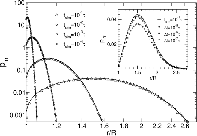
Figure 1: Morelli and ten Wolde

Results are collected in Figure 1: we simulate the irreversible reaction for 4 different simulation times, from $t_{\rm sim}\!=\!10^{-4}\tau$ to $t_{\rm sim}\!=\!10^{-1}\tau$, where $\tau\!=\!R^{2}/D$ is the natural time scale of the system. Particles are initially positioned at contact: $r_{0}\!=\!R$. We set the time step $\Delta t=10^{-4}t_{\rm sim}$, which corresponds to $P_{\rm acc,f}<0.14$. It is seen that both the shape and the area of the irreversible probability disitribution function is correctly captured by our algorithm. In the case of $t_{\rm sim}\!=\!10^{-1}\tau$, however, we needed to use $\Delta t=10^{-5}t_{\rm sim}$. In the Inset of Fig. 1, we show that in this last case, larger time steps lead our BD scheme to underestimate the survival probability. The deviation from the analytical results for large $\Delta t$ is due to the interplay bewteen a number of assumptions. One is that $1\!-\!\exp(P_{\rm acc,f})\simeq P_{\rm acc,f}$. A more important factor is that we compare the numerical results against analytical results of an analysis in which $k_{\rm on}$ corresponds to the intrinsic association rate for two particles that are at contact Kim and Shin (1998), while in our scheme the particles can already react when they are separated by a distance $\sim\sqrt{D\Delta t}$. This overestimates the number of reactions and hence decreases the survival probablity, consistent with the results shown in the inset of Fig. 1. Another way of putting this that in our BD algorithm, the intrinsic association rate is higher than that used in the analytical calculations.

III.2 Reversible Reactions

We extend now the dynamical test performed above to the case of the reversible reaction $A+B\overset{k_{\rm a}}{\underset{k_{\rm d}}{\rightleftharpoons}}C$. An analytical solution to the problem, $p_{\rm rev}(r,t|r_{0},t_{0})$ is known for one A and one B particle Kim and Shin (1998). In this test, we adopt the same setup and a similar procedure as for the irreversible case, except that we do not stop the run after a reaction, but we let the particle dissociate. At $t\!=\!t_{\rm{sim}}$ we check whether or not the $B$ particle is in the bound state. If it is not, we record the final position. The histogram of final positions of the $B$ particles is normalised to the number of survivors at $t\!=\!t_{\rm{sim}}$, and compared with the analytical curve $p_{\rm rev}(r,t_{\rm sim}|r_{0},0)$ Kim and Shin (1998). The fraction of runs ending in the unbound state yields an estimate for the survival probablity $S_{\rm rev}(t_{\rm sim}|r_{0})$. Again, we initially put the $B$ particle at contact ($r_{0}\!=\!R$), so that a larger number reactions and dissociations can happen within $t_{\rm{sim}}$. This choice will provide a stringent test for the dynamics of the system. The parameters of the system are the same as in Section III.1, with the addition of the dissociation rate $k_{\rm d}\!=\!1\tau^{-1}$. Similar results were obtained for larger values of $k_{\rm d}$, as well as for other values of $r_{0}$, $D$, and $k_{\rm a}$.

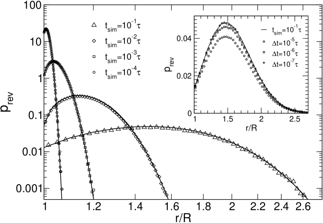
Figure 2: Morelli and ten Wolde

In Figure 2, we plot $p_{\rm rev}(r,t_{\rm sim}|R,0)$ for $t_{\rm{sim}}$ ranging from $10^{-1}\tau$ to $10^{-4}\tau$, with the same time steps as in the previous test. We find the BD algorithm correctly reproduces both the shape and the area of the analytical probability distribution. Similarly to Figure 1, we show in the Inset $p_{\rm rev}$, computed for $t_{\rm sim}\!=\!10^{-1}\tau$, for decreasing time steps $\Delta t$: as expected on the basis of the results for the irreversible reaction (Fig. 1), simulations with large time steps underestimate the survival probability.

For the next tests, we consider a setup similar to that used above, but we allow for multiple $B$ particles, and we enclose our system in a cubic simulation box of volume $V$, endowed with reflecting walls. All the $B$ particles can bind to the single $A$ particle, and do not interact among themselves. This last assumption, valid only in the limit of low packing fractions $\phi$, is satisfied in our simulations where $\phi\!<\!0.02$. Conversely, particles $B$ and $C$ interact as hard spheres, i.e. they are not allowed to overlap. We investigate whether equilibrium properties of the system, such as the probability of being in the bound state $C$ ($p_{\rm bound}$), are correctly reproduced by the BD algorithm. The probability $p_{\rm bound}$ can be evaluated by measuring the time when the $C$ particle is present in the system, with respect to the total simulation time. The mean field value for this quantity can be obtained from the macroscopic rate equation in steady state:

$$p_{\rm{bound}}=\frac{K_{\rm{eq}}N_{B}}{K_{\rm{eq}}N_{B}+V^{*}}\;,$$ (24)

where $K_{\rm{eq}}\!=\!k_{\rm a}/k_{\rm d}$, and $V^{*}=V\!-\!\frac{4}{3}\pi(R_{A}+R_{B})^{3}$. We note here that this prediction should be valid when the radial distribution at contact equals unity; given the low density of particles in our system this should be the case.

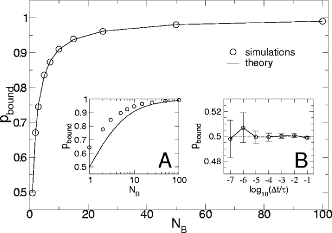
Figure 3: Morelli and ten Wolde

We simulate the system with a varying number $N_{B}$ of $B$ particles, with a fixed time step $\Delta t\!=\!10^{-4}\tau$. We choose $K_{\rm eq}\!=\!V$, so that $p_{\rm bound}(N_{B}\!=\!1)=0.5$. The enclosing box measures $(20R\times 20R\times 20R)$. Figure 3 compares the results of our simulations with the prediction of Eq. 24: we see a clear agreement. To illustrate that obeying the detailed-balance condition is important, we also performed a series of simulations in which the particles after dissociation were put at contact; in other words, we considered a function $g(r)=\delta(r\!-\!R)$. This move does violate detailed balance and indeed affects a correct estimate for $p_{\rm bound}$, as shown in Inset A of Figure 3: the incorrect procedure overestimates the time the particle spends in the bound state, especially for a low number of $B$ particles. These data clearly show that a naive treatment of the dissociation events leads to systematic errors, which are especially severe when the system has a low number of reactants, as it is often the case in biochemical networks. Finally, we tested whether the equilibrium properties of the system do not depend on the chosen time step. To this end, we compute $p_{\rm bound}$ for $N_{B}\!=\!1$ and different values of the time step $\Delta t$. As illustrated in the Inset B of Figure 3, we obtain a good agreement even for very large time steps, where probably the dynamics of the system is not entirely natural.

Finally, we compare our Brownian Dynamics algorithm with the Stochastic Simulation Algorithm, based on a Kinetic Monte Carlo scheme that propagates the system according to the solution of its zero-dimensional chemical master equation Gillespie (1977). This scheme accounts only for the stochasticity arising from the fluctuations in the number of particles; spatial fluctuations due to the diffusive motion of particles are completely neglected. The system is thus assumed to be well-stirred at all times. We consider the reversible reaction $A+B\rightleftharpoons C$ for $N_{B}\!=\!1$: in the SSA, the association times follow a Poisson distribution, with mean $1/k_{\rm f}$, where $k_{\rm f}^{-1}=1/(4\pi DR)\!+\!k_{\rm a}^{-1}$ is the macroscopic forward rate.

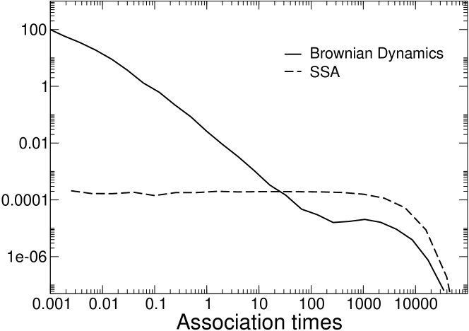
Figure 4: Morelli and ten Wolde

We collect the association times for a BD run with $V\!=\!64000R^{3},\Delta t\!=\!10^{-4}\tau,k_{\rm a}\!=\!100R^{3}/\tau,k_{\rm off}\!=\!1000\tau^{-1}$, and we compare it with an SSA run obtained with the same set of parameters, but using the modified association rate $k_{\rm f}$. Figure 4 compares the two distributions: the BD line shows a marked increase in the number of association events at short times, as compared to the Poissonian distribution with mean $k_{\rm f}$ of the SSA. This effect has a purely spatial origin and has been previously observed (Zon and ten Wolde (2005); van Zon et al. (2006)): when particles dissociate in space, their distance is still very small, therefore the probability of an immediate rebinding in next few times steps is very high. Long association times, in a BD simulation, are related to particles which have wandered diffusively in the box, and have finally found the target. The distribution of such times is again exponential, with a constant $k_{\rm f}$.

The test above show that our BD algorithm, which rigorously obeys detailed balance, correctly reproduces the equilibrium properties and provides a good description of the dynamics of the system in time and space.

IV Application: the push-pull model

In this Section, we apply our Brownian Dynamics to a simple model of a push-pull network. In this network, two antagonistic enzymes continually covalently modify and demodify a substrate, respectively; a well-known example is a protein that is phosphorylated and dephosphorylated by a kinase and a phosphatase, respectively. The first enzyme converts a substrate molecule into an “active” state: bearing in mind the phosphorylation example, we call this active substrate $S_{p}$, and the enzyme $K$ (kinase). A molecule in the active state $S_{p}$ can be brought back to the original state $S$ under the action of a second enzyme, $P$ (phosphatase). The model is nicknamed “push-pull”, as the substrates are continuously switching between the two states, while consuming energy. The reactions with the enzymes are described according to Michaelis-Menten kinetics: the two reactants form first an intermediate bound state, which can lead either to a dissociation or to the release of a converted molecule. In Goldbeter and D. E. Koshland (1981), the model is solved at the level of the Macroscopical Rate Equation at steady state, which yields the average behavior of the system.

Goldbeter and Koshland showed that such a system can display an ultrasensitive behavior (that is, a sensitivity curve steeper than the conventional response showed by the Michaelis-Menten mechanism) without the need of introducing cooperative interactions Goldbeter and D. E. Koshland (1981). More precisely, the interplay between two converter enzymes operating in opposite directions on a target whose quantity is conserved can give rise to a switch-like response in the steady-state fraction of modified molecules, when the ratio between the conversion rates is varied. The requirement for such a sharp transition is the saturation of the enzymes: the effective conversion rates then become independent on the number of substrate molecules, thus making the reaction rates “zero-order” in the substrate concentration.

The above-mentioned analysis does not however account for any kind of fluctuations that may arise from the low number of reactants, the stochastic behavior of the chemical reactions, or the diffusion of the molecules in space. In Berg et al. (2000), the same model is studied at the level of the chemical master equation, taking into account finite-size effects that arise in real systems, that is the discreteness and the possible low copy number of enzymes and substrates. In order to achieve ultrasensitivity, the enzymes must be saturated, and therefore their concentration is likely to be very low. Large fluctuations are then observed around their average behavior: the authors show that the results obtained with a mesoscopic approach reduce to those of the macroscopic analysis of Goldbeter and D. E. Koshland (1981) only when the number of molecules is sufficiently large. If this is not the case, as it can easily happen in a bacterial cell where some species are present only in few dozens of copies, the sensitivity of the system is reduced, and the response is less steep than the macroscopic theory would predict. This deviation can be easily understood when one realises that high sensitivity corresponds to highly saturated enzymes. In this regime, the reaction rates do not depend on the number of substrate molecules. The system performs a random walk in the number of $S$ molecules and it is thus subject to large fluctuations. Our Brownian Dynamics algorithm now allows us to study the effect of spatial fluctuations due to the diffusive motion of the molecules.

The system we consider is defined by the following set of reactions:

$$\mathrm{Reaction} \mathrm{Rate}$$

$$S+K\rightleftharpoons KS k_{\rm on1},\>k_{\rm off1}$$ (25a)

$$KS\to K+S_{p} k_{1}$$ (25b)

$$S_{p}+P\rightleftharpoons PS_{p} k_{\rm on2},\>k_{\rm off2}$$ (25c)

$$PS_{p}\to P+S k_{2}.$$ (25d)

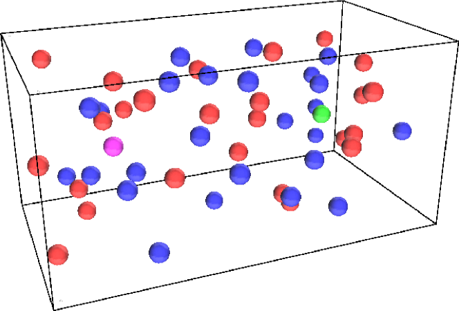
Figure 5: Morelli and ten Wolde

Here $k_{\rm f}$ stands for the macroscopical association rate. The system will be simulated with the BD algorithm in a rectangular box of dimensions $x_{\rm box}\!=\!20R,y_{\rm box}\!=\!10R,z_{\rm box}\!=\!10R$, with a single kinase and a single phosphatase molecule, held fixed at distance $\Delta\!=\!0.5x_{\rm box}$ on the central axis of the box, as depicted in Figure 5. The system is initially prepared with $N_{S\rm tot}$ particles, distributed in the two states according to the solution of the macroscopical rate equation. In the following, we investigate the effect of spatial fluctuations of the substrate molecules on the input-output relation of the system, and we compare the BD results to those obtained with the mean-field and the zero-dimensional chemical master equation approach.

The input-output relation is defined as the mean fraction of phosphorylated substrate molecules $\langle S_{p}\rangle/N_{S\rm tot}$ as a function of the ratio $k_{1}/k_{2}$. We compute it with 80 substrate molecules in the simulation box, in order to meet the requirement $N_{S}\!\gg\!N_{K}$ and $N_{S_{p}}\!\gg\!N_{P}$ $(N_{S}\!+\!N_{S_{p}}=N_{S\rm tot})$. The parameters governing the steepness of the sigmoid curves are the Michaelis-Menten equilibrium rates $K_{1}\!=\!(k_{\rm off1}+k_{1})/k_{\rm on1}$ and $K_{2}\!=\!(k_{\rm off2}+k_{2})/k_{\rm on2}$. In all our simulations we set $K_{1}\!=\!K_{2}\!=\!K_{\rm M}$. In our simulations, diffusion constants are in the order of $10^{-4}-10^{-5}R^{2}/\Delta t$, intrinsic association rates between 0.001 and 0.006 $R^{3}/\Delta t$, dissociation rates vary between $5\cdot 10^{-4}$ and $5\cdot 10^{-6}(\Delta t)^{-1}$, and production rates are chosen in the range $10^{-4}-10^{-8}(\Delta t)^{-1}$. To vary $k_{1}/k_{2}$ keeping $K_{\rm M}$ constant, we vary $k_{\rm off1}$ and $k_{\rm 1}$ together, keeping their sum constant. When $K_{\rm M}/[S_{\rm tot}]\ll 1$ the enzymes are totally saturated and the change in the fraction of modified proteins is abrupt; on the other hand, when $K_{\rm M}/[S_{\rm tot}]\geq 1$, the rise of the curve becomes asymptotically close to the hyperbolic Michaelis-Menten shape.

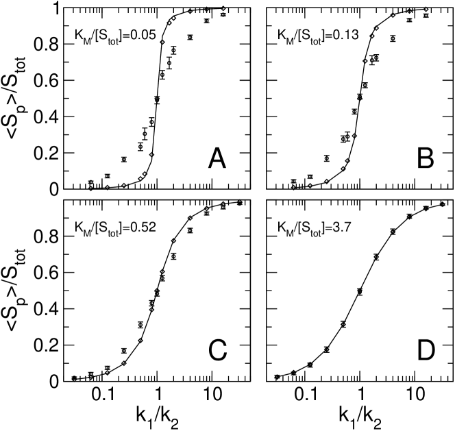
Figure 6: Morelli and ten Wolde

Figure 6 shows several examples of the input-output relation, obtained with three different methods: with the analytic macroscopic approach of Goldbeter and D. E. Koshland (1981) (solid lines), with SSA simulations as in Berg et al. (2000) (diamonds) and with the Brownian Dynamics algorithm (circles). The BD simulations are performed with intrinsic association and dissociation rates $k_{\rm a}$ and $k_{\rm d}$, respectively. In the mean-field analysis and the SSA simulations of the zero-dimensional chemical master equation, for the association reaction the rate constant was chosen to be that of the macroscopic association rate $k_{\rm on}$, as given by $k_{\rm on}=(1/k_{\rm a}\!+\!1/k_{\rm D})^{-1}$, with $k_{\rm a}$ being the intrinsic association rate, and $k_{\rm D}=4\pi RD$ the diffusion-limited rate (see Eq. 5). For the rate constant of the backward reaction in the mean-field analysis and the SSA simulations, we chose the intrinsic reaction rate and not the macroscopic one given by Eq. 6. The reason is that the macroscopic dissociation rate takes into account that, upon dissociation, the dissociated species rebind a number of times before they diffuse away from each other into the bulk van Zon et al. (2006). As we have recently shown, association and dissociation reactions can be described with effective rates given by Eqs. 5 and 6 when the associated species can only dissociate, thus when there is no competing decay channel for the associated species van Zon et al. (2006). In particular, in Ref. van Zon et al. (2006) we studied the effect of spatial fluctuations due to the diffusive motion of repressor molecules on the noise in the expression of a gene; the simulation results showed that the stochasticity in the binding of the repressor to the DNA resulting from the spatial fluctuations of the repressor molecules can be a major source of noise in gene expression; however, this result could be described by renormalising the intrinsic association and dissociation rates for repressor-DNA binding using the expressions of Eq. 5 and Eq. 6. Here, the situation is markedly different. The reason is that the associated species, $KS$ and $PS_{p}$, can either dissociate or lead to a chemical modification reaction, upon which the product must diffuse to the other enzyme in order to be demodified. These reaction channels compete with one another, and if they compete with one another on the same time scale, the effective dissociation rate is difficult to determine. In our system, however, the number of rebindings is in the order of unity. Therefore, renormalising the rate constants does not substantially change the actual values of the rate constants. We carried out simulations where we chose either to renormalise both the association and dissociation rates or neither of them, and we found analogous results. In the following, we show only BD data obtained with the intrinsic dissociation and association rate. $K_{\rm M}$ is computed with the intrinsic dissociation rates, and and with $k_{\rm on}=(k_{\rm D}^{-1}+k_{\rm a}^{-1})^{-1}$.

The different panels of Figure 6 show the data for increasing $K_{\rm M}/[S_{\rm tot}]$. In panel D, $K_{\rm M}/[S_{\rm tot}]\!=\!3.7$ and the response of the system is very similar to a Michaelis-Menten kinetics. In this case, the results of the simulations, obtained both with BD and the SSA, perfectly follow the analytical curve. When $K_{\rm M}\!>\!1$, both reactions are in the first-order regime, which means that their rates are proportional to the number of substrate molecules. As a result, when this number changes, the rates of conversion in the opposite direction changes immediately. This counteracts the modification and reduces the effect of fluctuations. However, as we decrease $K_{\rm M}$, the numerical data start to deviate from the predicted macroscopic behaviour. In the case of SSA, the deviation is mild, and barely visible in panel A, where $K_{\rm M}/[S_{\rm tot}]\!=\!0.05$. In contrast, the BD simulations yield a much more marked deviation, clearly seen already from panel C, where $K_{\rm M}/[S_{\rm tot}]\!=\!0.52$.

The data in Figure 6 confirm and extend the findings of Ref. Berg et al. (2000): stochastic fluctuations of the system dampen the ultrasensitivity, which could be obtained only in an infinitely large, well-stirred system. The SSA correctly accounts for the temporal fluctuations arising from the stochastic behavior of chemical reactions, and for the discreteness of the components, but it does assume a well-stirred system, where spatial fluctuations can be neglected. These hypothesis result in a deviation on the order of few per cents in the ultrasensitive regime. Brownian Dynamics, on the contrary, properly accounts for temporal and spatial fluctuations. These last are related to the diffusive motion of the substrate molecules; when the concentrations of the species are low, they become a serious limiting factor which notably reduces the sensitivity of system. Brownian Dynamics is therefore able to show that the response of the system can be much less sensitive than predicted at the macroscopic level in the ultrasensitive regime, if the species move slowly enough in space, i.e. when the system is not well-stirred.

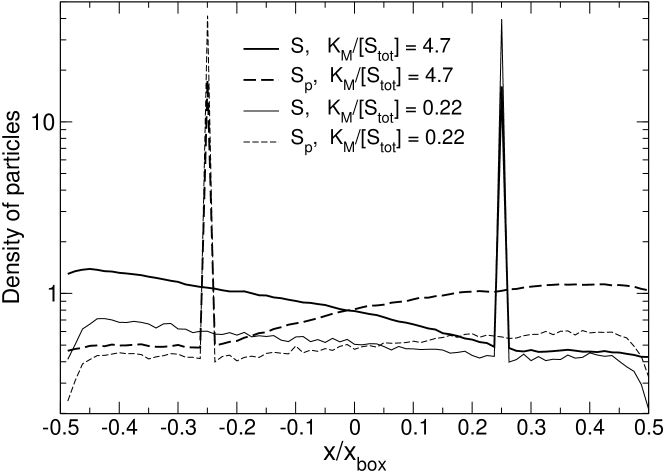
Figure 7: Morelli and ten Wolde

Finally, we emphasise that Brownian Dynamics algorithms can be used to directly measure spatial properties of the system. Among several possibilities, we choose to show in Figure 7 the spatial density of particles along the main axis of the box. Data are obtained for two different values of the Michaelis-Menten constant: $K_{\rm M}/[S_{\rm tot}]\!=\!4.7$ ($D=10^{-4}R^{2}/\Delta t,k{\rm on}=0.007R^{3}/\Delta t,k_{1}+k_{\rm off1}=2\cdot 10^{-4}(\Delta t)^{-1},N_{S_{\rm tot}}=80$), where the system is in the first-order regime, and $K_{\rm M}/[S_{\rm tot}]\!=\!0.22$ ($D=10^{-3}R^{2}/\Delta t,k_{\rm on}=0.01R^{3}/\Delta t,k_{1}+k_{\rm off1}=5\cdot 10^{-5}(\Delta t)^{-1},N_{S_{\rm tot}}=80$), corresponding to the ultrasensitive regime. Substrate molecules are very often bound to the enzymes: at the kinase enzyme, the $S$ density has a sharp peak, and so does the $S_{p}$ density at the location of the phosphatase enzyme. The height of the peak is bigger when the system is simulated for a low value of $K_{\rm M}$, where enzymes are completely saturated. Interestingly, the concentration of both molecules shows a gradient along the $x$ direction, higher in the half box where the molecules are produced. Such gradient is not particularly appreciable for low values of $K_{\rm M}$: in this regime, enzymes are saturated and dissociation events are rare. The particles have therefore the time to spread in the box and reach an homogeneous concentration only occasionally perturbed by a production event. For high values of $K_{\rm M}$, particles are produced more often and they do not have the time to stir in the box, leading to an accumulation close to the production sites. The profiles for the two species are completely symmetric, as these simulations are obtained for $k_{1}\!=\!k_{2}$. Naturally, such a spatial property could not be captured if the system is simulated at the level of the zero-dimensional chemical master equation.

V Discussion

In this manuscript, we have presented a Brownian Dynamics algorithm that rigorously obeys detailed balance for equilibrium reactions. Consequently, the equilibrium properties of biochemical networks, such as promoter and receptor occupancies, are reproduced exactly to within the statistical error. Moreover, the association and dissociation reaction moves are constructed such that they allow for a meaningful interpretation: as the time step $\Delta t\to 0$, the association and dissociation rates approach the intrinsic values corresponding to the reaction rates of the species at contact. This is useful, also because it allows the BD results to be compared to theoretical results on diffusion-influenced reactions, which describe reactions as reactions between species at contact Agmon and Szabo (1990). The results shown in Figs. 1 and 2 show that as $\Delta t\to 0$, the BD simulations correctly describe not on the equilibrium properties, but also the dynamical properties of a bimolecular reaction. For larger time steps, the BD results deviate from the analytical results, but this is to be expected since the analytical results assume that the molecules move by diffusion up to the smallest length and time scales, and that reactions only occur once the molecules have moved by diffusion into contact. We believe that while the BD results and the analytical results match for $\Delta t<10^{-6}R^{2}/D$ (Figs. 1 and 2), the BD algorithm gives a good description of the dynamics over a large range of time steps, i.e. for $\Delta t<10^{-4}$, because in this range the BD results can be fitted to the analytical results with a different $k_{\rm a}$ and $k_{\rm d}$ (data not shown).

As an illustrative example, we have applied our BD scheme to a model representing the dynamics of a substrate molecule under the action of two antagonistic enzymes. This model was previously analysed with deterministic methods Goldbeter and D. E. Koshland (1981), which revealed an ultrasensitive behavior in the response of the system when the enzymes are fully saturated. A study conducted at the level of the Chemical Master Equation Berg et al. (2000), thus accounting for the low copy number of the substrate molecules, highlighted that the ultrasensitivity predicted in Ref. Goldbeter and D. E. Koshland (1981) cannot be achieved when the concentration of the substrate is very low. Temporal fluctuations limit then the sensitivity of the system in the ultrasensitive regime. We repeated the analysis of Ref. Berg et al. (2000) simulating the system with the SSA, and confirmed their findings. Furthermore, we have investigated the role of spatial fluctuations on the system with BD simulations. Our analysis shows that the sensitivity of the response curve in the ultrasensitive regime is furtherly reduced when the diffusion of the reactants is taken into account explicitely. In particular, when the diffusion of particles is slow and the system is far from well-stirred, spatial fluctuations are the dominant source of noise, and the reduction in the gain is significant.

Appendix A Detailed balance for a well-stirred model

In the case of the well-stirred model we used in Sec. III.2 and IV, the detailed-balance condition is simpler than in the spatially resolved model. Let $N_{A},N_{B},N_{C}$ be the number of $A$, $B$ and $C$ molecules and $V$ the volume of the system. The configurational partition function of the system can be written as the following sum of terms in the canonical ensemble:

$${\cal Q}=\sum_{\{N\}}Q(N_{A},N_{B},N_{C}),$$ (26)

where $\{N\}$ denotes all possible combinations of $\{N_{A},N_{B},N_{C}\}$; note that we integrated here over the momenta. The choice of the canonical ensemble is motivated by the assumption that the cell is a closed system, and it does not exchange particles with the environment.

Let us consider the case where $\{A,B,C\}$ are ideal particles in a volume $V$, except for the fact, of course, that $A$ and $B$ can form $C$. The configurational integral $Q$ for $\{N_{A},N_{B},N_{C}\}$ particles is then:

$$Q(N_{A},N_{B},N_{C}) = \frac{q_{A}^{N_{A}}q_{B}^{N_{B}}q_{C}^{N_{C}}}{N_{A}!N_{B}!N_{C}!}$$

$$= \frac{q_{A,\rm{cm}}^{N_{A}}q_{B,\rm{cm}}^{N_{B}}q_{C,\rm{cm}}^{N_{C}}}{N_{A}!N_{B}!N_{C}!}V^{N_{A}+N_{B}+N_{C}},$$

where $q_{A}$ is the molecular partition function for an $A$ particle, and the factor $1/(N_{A}!)$ takes into account the indistinguishability of the $A$ particles. The molecular partition function is given by $q_{A}\!=\!q_{A}^{\rm id}q_{A,\rm{cm}}$, where $q_{A,\rm{cm}}$ is the partition function corresponding to the internal degrees of freedom relative to the center of mass and $q_{A}^{\rm id}\!=\!V$ is the partition function associated with the translational degrees of freedom of the center of mass. The probability that the system has $\{N_{A},N_{B},N_{C}\}$ molecules, $P(N_{A},N_{B},N_{C})$, is then:

$$P(N_{A},N_{B},N_{C})=Q(N_{A},N_{B},N_{C})/{\cal Q}.$$ (28)

Let us now consider the transition from $\{N_{A},N_{B},N_{C}\}$ to $\{N_{A}-1,N_{B}-1,N_{C}+1\}$ molecules. The ratio between the probabilities of being in the state after and before the transition is:

$$\frac{P(N_{A}-1,N_{B}-1,N_{C}+1)}{P(N_{A},N_{B},N_{C})} = \frac{N_{A}N_{B}}{N_{C}+1}\frac{1}{V}\frac{q_{C,\rm cm}}{q_{A,\rm cm}q_{B,\rm cm}}.$$ (29)

$$= \frac{N_{A}N_{B}}{N_{C}+1}\frac{1}{V}K_{\rm eq}=\frac{N_{A}N_{B}}{N_{C}+1}\frac{1}{V}\frac{k_{\rm f}}{k_{\rm b}}.$$ (30)

Please note that $K_{\rm eq}$ has dimension of volume, such that the expression on the right-hand-side is indeed dimensionless. The above expression serves to illustrate the detailed-balance rule Frenkel and Smit (2002), which states that

$$P_{\rm unbound}P_{\rm u\to b}=P_{\rm bound}P_{\rm b\to u}.$$ (31)

Here $P_{\rm unbound}$ is the probability of being in the state $\{N_{A},N_{B},N_{C}\}$, $P_{\rm u\to b}$ is the probability of a transition from $\{N_{A},N_{B},N_{C}\}$ to $\{N_{A}-1,N_{B}-1,N_{C}+1\}$, $P_{\rm b\to u}$ is the probability of the reverse move, and $P_{\rm bound}$ is the probability of being in the state $\{N_{A}-1,N_{B}-1,N_{C}+1\}$. Using Eq. (30) and the former relation we obtain:

$$P_{\rm u\to b}=\frac{k_{\rm f}}{V}N_{A}N_{B}\quad{\rm and}\quad P_{\rm b\to u}=k_{\rm b}(N_{C}+1).$$ (32)

These transition probabilities precisely correspond to those used in Monte Carlo simulations of the zero-dimensional chemical master equation Gillespie (1977).

Appendix B Derivation of $g(r)$

The function $g(r)$, described in Section II is given by the integral of equation (20):

$$g(r)=\frac{1}{(\pi\sigma^{2})^{3/2}}\int_{0}^{R}r^{\prime 2}dr^{\prime}\int_{0}^{\pi}\sin\theta d\theta\int_{0}^{2\pi}d\varphi\,\exp\left(-\frac{r^{\prime 2}-2rr^{\prime}\cos\theta+r^{2}}{\sigma^{2}}\right),$$ (33)

where $\sigma^{2}=4D\Delta t$.
Elementary methods can be used: integration over the angular variables yields

$$g(r)=\frac{1}{\sqrt{\pi\sigma^{2}}}\frac{\exp{\left(-r^{2}/\sigma^{2}\right)}}{r}\int_{0}^{R}\left[\exp\left(-\frac{r^{\prime 2}-2rr^{\prime}}{\sigma^{2}}\right)-\exp\left(-\frac{r^{\prime 2}+2rr^{\prime}}{\sigma^{2}}\right)\right]r^{\prime}\,dr^{\prime}.$$ (34)

Integrating over all the possible final positions corresponding to an overlap between the particles ($0\!\leq\!r^{\prime}\!\leq\!R$), gives

$$g(r)=\frac{\sigma}{\sqrt{\pi}}\frac{1}{2r}\left[\exp\left(-\frac{(r+R)^{2}}{\sigma^{2}}\right)-\exp\left(-\frac{(r-R)^{2}}{\sigma^{2}}\right)\right]+\frac{1}{2}\left[\rm{erf}\left(\frac{r+R}{\sigma}\right)+\rm{erf}\left(\frac{-r+R}{\sigma}\right)\right],$$ (35)

where

$$\rm{erf}(x)=\frac{2}{\sqrt{\pi}}\int_{0}^{x}e^{t^{2}/2}dt.$$

1. Radial probability distribution for an irreversible reaction. The four curves refer to different $t_{\rm{sim}}$ and were obtained with time steps $\Delta t\!=\!10^{-4}t_{\rm{sim}}$, except for $t_{\rm sim}\!=\!0.1\tau$ where we used $\Delta t\!=\!10^{-5}t_{\rm{sim}}\!=\!10^{-6}\tau$ ($\tau\!=\!R^{2}/D$, $R\!=\!R_{A}\!+\!R_{B}$). Particles were initially positioned at contact: $r_{0}\!=\!R$. The intrinsic association constant is $k_{\rm a}\!=\!1000R^{3}/\tau$. The numerical results (symbols) are in excellent agreement with the analytical curves (solid lines) Kim and Shin (1998). In the Inset, we plot the probability distribution for $t_{\rm sim}\!=\!10^{-1}\tau$ for several time steps. For large $\Delta t$ the BD algorithm deviates from the analytical line and underestimates the survival probability. Error bars are smaller than symbol sizes.

2. Radial probability distribution for a reversible reaction. The four curves refer to different $t_{\rm{sim}}$ and were obtained with time steps $t_{\rm{step}}\!=\!10^{-4}t_{\rm{sim}}$, $r_{0}\!=\!R$, except for $t_{\rm sim}\!=\!0.1\tau$ where we used $\Delta t\!=\!10^{-5}t_{\rm{sim}}\!=\!10^{-6}\tau$ ($\tau\!=\!R^{2}/D$, $R\!=\!R_{A}+R_{B}$). Particles were initially positioned at contact ($r_{0}\!=\!R$), and the association rate constant is $k_{\rm a}\!=\!1000R^{3}/\tau$ ($\tau\!=\!R^{2}/D$, $R\!=\!R_{A}+R_{B}$), while the dissociation rate constant is set to $k_{\rm d}\!=\!1\tau^{-1}$. The numerical results (circles) agree with the analytical curves (solid lines). In the Inset, the probability distribution for $t_{\rm sim}\!=\!10^{-1}\tau$ is plotted for several values of $\Delta t$: for large values of the time step, the BD algorithm deviates from the analytical line and underestimates the survival probability. Error bars are smaller than symbol sizes.

3. Probability of having an $A$ particle bound to a $B$ particle, as a function of the number of $B$ particles. The time step is set to $\Delta t\!=\!10^{-4}\tau$ ($\tau\!=\!R^{2}/D$, $R\!=\!R_{A}+R_{B}$), the intrinsic association constant to $k_{\rm on}\!=\!71R^{3}/\tau$ so that $P_{\rm acc,\,f}\!=\!0.1$. $k_{\rm b}$ is chosen so that $K_{\rm eq}\!=\!k_{\rm f}/k_{\rm b}\!=\!V$ ($V\!=\!8000R^{3}$) and therefore $p_{\rm bound}(N_{B}\!=\!1)\!=\!0.5$. The numerical data obtained with BD are in agreement with the mean-field values. The error bars of the numerical results are smaller than the size of the circles. In Inset A, the simulations are performed positioning dissociated particles at contact. This move violates detailed balance and yield an incorrect $p_{\rm bound}$ for low number of particles. In Inset B, $p_{\rm bound}$, for $N_{B}\!=\!1$ is plotted against the time step used in the simulations. To keep $P_{\rm acc,\,f}\!=\!0.1$, we varied $k_{\rm on}$ from $2242R^{3}/\tau$ ($\Delta t\!=\!10^{-7}\tau$) to $0.00026R^{3}/\tau$ ($\Delta t\!=\!10^{-1}\tau$). As expected for an equilibrium quantity, $p_{\rm bound}$ does not depend on the chosen time step.

4. Distribution of association times, for the reaction $A+B\leftrightarrow C$, obtained with the Brownian Dynamics algorithm (solid line) and with a Stochastic Simulation Algorithm (dashed line) neglecting spatial effects. The data are obtained for $V\!=\!64000R^{3},D\!=\!R^{2}/\tau,\Delta t\!=\!10^{-4}\tau,k_{\rm a}\!=\!100R^{3}/\tau,k_{\rm d}\!=\!1000\tau^{-1}$ ($\tau\!=\!R^{2}/D$, $R\!=\!R_{A}+R_{B}$). Spatial simulations account for immediate rebindings after a dissociation event, and show a higher probability for short association times. The two curves decay exponentially to zero with the same rate $k_{\rm f}^{-1}=k_{\rm a}^{-1}\!+\!k_{\rm D}^{-1}$.

5. Snapshot of the push-pull system. The pink and the green sphere represent, respectively, the kinase and the phosphatase molecule, held fixed along the main axis of the box. The blue and red spheres represent $S$ and $S_{p}$ molecules, respectively. The system is represented for $N_{S\rm tot}\!=\!50$ and a box of $20R\times 10R\times 10R$.

6. Fraction of converted molecules as a function of ratio of the convertion rates $k_{1}/k_{2}$. The data are shown for increasing values of $K_{\rm M}/[S_{\rm tot}]$ from panel A to D. Panel A corresponds to full saturation of enzymes, whereas in panel D the system is in the first-order regime. The continuous lines are obtained by solving the Macroscopical Rate Equation, whereas diamonds correspond to the numerical solutions of the master equation (obtained with the conventional SSA) and circles to the output of our BD simulations. SSA data (error bars are smaller than the sizes of the symbols) show a mild deviation only when the system displays an ultrasensitive behavior, as in panel A. Brownian Dynamics simulations deviate notably from the macroscopic curve when $K_{\rm M}/[S_{\rm tot}]\!<\!1$. Methods accounting for the stochastic behavior of the system show thus a reduction in sensitivity for low values of $K_{\rm M}\!$. In the simulations, we vary $k_{1}$ and $k_{\rm off2}$ keeping their sum constant, so that $k_{1}/k_{2}$ is varied while $K_{\rm M}$ does not change. For all panels, $D=10^{-3}R^{2}/(\Delta t),N_{S_{\rm tot}}=80$. Panel A: $k_{1}+k_{\rm off1}=k_{2}+k_{\rm off2}=5\cdot 10^{-6}\Delta t^{-1}$, $k_{\rm a}=0.006R^{3}/(\Delta t)$. Panel B: $k_{1}+k_{\rm off1}=k_{2}+k_{\rm off2}=5\cdot 10^{-6}\Delta t^{-1}$, $k_{\rm a}=0.001R^{3}/(\Delta t)$, Panel C: $k_{1}+k_{\rm off1}=k_{2}+k_{\rm off2}=5\cdot 10^{-5}\Delta t^{-1}$, $k_{\rm a}=0.003R^{3}/(\Delta t)$, Panel D: $k_{1}+k_{\rm off1}=k_{2}+k_{\rm off2}=2\cdot 10^{-4}\Delta t^{-1}$, $k_{\rm a}=0.0015R^{3}/(\Delta t)$.

7. The spatial density profiles for $S$, $S_{p}$ ($k_{1}/k_{2}\!=\!1$) show clear symmetric peaks around the locations of the two enzymes: respectively, the $S$ density is peaked around the kinase enzyme, at $x\!=\!0.25x_{\rm box}$, and the $S_{p}$ density around the phosphatase at $x\!=\!-0.25x_{\rm box}$. These peaks are more pronounced when the system is in the ultrasensitive regime (thinner lines). Moreover, for high values of the Michaelis-Menten constants (thicker lines), the spatial density of the particles show a gradients, higher close to the production sites of the molecules. For low values of $K_{\rm M}$ the gradients are not appreciable anymore: the particles can diffuse in the box and reach an homogeneous distribution, as production events happen on slow time scales. Simulation parameters: $K_{\rm M}/[S_{\rm tot}]=4.7,D=10^{-4}R^{2}/(\Delta t),N_{S_{\rm tot}}=80,k_{1}=k_{2}=k_{\rm off1}=k_{\rm off2}=10^{-4}\Delta t^{-1},k_{\rm a}=0.007R^{3}/(\Delta t)$ $K_{\rm M}/[S_{\rm tot}]=0.22,D=10^{-3}R^{2}/(\Delta t),N_{S_{\rm tot}}=80,k_{1}=k_{2}=k_{\rm off1}=k_{\rm off2}=2.5\cdot 10^{-5}\Delta t^{-1},k_{\rm a}=0.01R^{3}/(\Delta t)$