Ground-state properties of interacting two-component Bose gases in a one-dimensional harmonic trap

Abstract

We study ground-state properties of interacting two-component boson gases in a one-dimensional harmonic trap by using the exact numerical diagonalization method. Based on numerical solutions of many-body Hamiltonians, we calculate the ground-state density distributions in the whole interaction regime for different atomic number ratio, intra- and inter-atomic interactions. For the case with equal intra- and inter-atomic interactions, our results clearly display the evolution of density distributions from a Bose condensate distribution to a Fermi-like distribution with the increase of the repulsive interaction. Particularly, we compare our result in the strong interaction regime to the exact result in the infinitely repulsive limit which can be obtained by a generalized Bose-Fermi mapping. We also discuss the general case with different intra- and inter-atomic interactions and show the rich configurations of the density profiles.

I Introduction

The realization of two-component Bose-Einstein condensates (BECs) of trapped alkali atomic clouds Myatt ; Erhard has stimulated the great interest in the multi-component atomic (or spinor) gases. The competition between inter-species and intra-species interactions gives rise to a richer structure of spinor condensates than their single component counterparts. Many theoretical investigations have focused on its stability, phase separation, collective excitation, dynamics and other macroscopic quantum phenomena Ho96 ; Ao ; Pu ; Cazalilla . Moreover resonant control of two-body interactions via Feshbach resonances in ultracold gases makes it possible to study a two-component condensate with a tunable interspecies interaction. On the other hand, the experimental progress in the creation and manipulation of ultracold atomic gases in effective one-dimensional (1D) waveguides Stoeferle ; Paredes ; Toshiya offers the opportunity of studying the many-body physics of the 1D correlated quantum gases even in the strong interaction limit. The experimental realization of Tonks-Girardeau (TG) gases Girardeau in the strongly interacting limit of Bose gases has been reported in two recent experiments Paredes ; Toshiya .

For the 1D quantum gases Olshanii , quantum fluctuations are greatly enhanced and the effects of strong correlations become very important Olshanii2 ; Petrov ; Dunjko ; Chen . Although two-component quantum gases have been the subject of intensive theoretical interest Ho96 ; Ao ; Pu ; Cazalilla , most of the studies were carried out within the scheme of the mean field theory which are proven insufficient for strong interactions between particles. For the system in the strong interaction regime, non-perturbation theory has to be exerted. For the 1D homogeneous system with $\delta$-function interaction, the two-component Bose gas with spin-independent s-wave scattering (equal interspecies and intra-species interacting strength) is known to be exactly solvable by the Bethe-ansatz method in the full physical regime LiYQ . The exact results have unveiled that ferromagnetic order emerges in spinor Bose gases with spin-independent interaction Eisenberg ; LiYQ ; Guan07 ; Fuchs . But for the atomic gases with arbitrary interacting strength (with the SU(2) symmetry broken) or in an inhomogeneous trap, the system is no longer integrable.

Despite no exact solution for the many-body systems with arbitrary interacting strength in a harmonic trap available, it is still possible to resort to numerical exact diagonalization method to obtain the exact solution for small size system. Most recently, some sophistical theoretical methods, such as the exact diagonalization method Deuretzbacher ; Yin and multi-orbital self-consistent Hartree method Zoellner ; Zoellner06 ; Cederbaum ; Cederbaum06 have been applied to study the single-component few-boson systems in a harmonic trap. Due to properly accounting the many-body effects, such methods work well even in strongly interacting regime and yield consistent results with the exact results obtained by the Bethe-ansatz method Hao06 ; Hao07 . In this work, we shall study two-component boson systems with repulsive interactions and focus on few-atom systems which can be treated exactly by exact diagonalization method. One of the purpose of the present work is to address the role of the correlation in the trapped interacting two-component system under a well controllable way, in particular in the strongly interacting limit where the approximate mean-field methods are generally not able to give correct results. Our study can display the transition from a weakly interacting condensate to the strongly interacting limit in which the strongly repulsive interactions between atoms plays a role of effective Pauli principle. In this limit, we compare our result with the exact result in TG-gas limit via a generalized Bose-Fermi mapping which has been applied to the Bose-Fermi mixtures by Girardeau et. al very recently Girardeau07 . We also address the case with different inter-species and intra-species interactions.

Our paper is organized as follows. Section II introduces the model and gives a brief introduction to the computational method. The subsequent section is devoted to our results for the ground-state density distribution. A summary is given in the last section.

II The microscopic model and the method

Let us consider the two components of Bose gases confined in a strongly anisotropic harmonic trap, where the transverse confinement frequency $\omega_{\perp}$ is strong enough so that the dynamics of Bose gases are effectively described by a 1D model due to the radial degrees of freedom are frozen. We start with the microscopic Hamiltonian of two species of Bosons

$$H = \int dx\sum_{\alpha=1,2}\left\{\Psi_{\alpha}^{\dagger}(x)\left[-\frac{\hbar^{2}}{2m_{\alpha}}\frac{\partial^{2}}{\partial x^{2}}+V_{\alpha}(x)\right]\Psi_{\alpha}(x)\right.$$ (1)

$$\left.+\frac{g_{\alpha}}{2}\Psi_{\alpha}^{\dagger}(x)\Psi_{\alpha}^{\dagger}(x)\Psi_{\alpha}(x)\Psi_{\alpha}(x)\right\}$$

$$+g_{12}\int dx\Psi_{1}^{\dagger}(x)\Psi_{2}^{\dagger}(x)\Psi_{2}(x)\Psi_{1}(x)$$

with $V_{\alpha}(x)=\frac{1}{2}m_{\alpha}\omega_{\alpha}^{2}x^{2}$ ($\alpha=1,2$) being the trap potential felt by the $\alpha$-component bosons with mass $m_{\alpha}$ and longitudinal trap frequency $\omega_{\alpha}$. Here $\Psi_{\alpha}(x)$ denotes the field operator of the $\alpha$-component bosons for the longitudinal degree of freedom. In the following we will focus on the two-component Bose gases composed of two hyperfine state of the same atoms such that $m_{1}=m_{2}=m$ and it is assumed that both of them feel the same trap frequency, i.e., $\omega_{1}=\omega_{2}=\omega$. The effective intra- and inter-atomic interaction strengths are denoted as $g_{\alpha}=-2\hbar^{2}/(ma_{1d}^{\alpha})$ ($\alpha=1,2$) and $g_{12}=-2\hbar^{2}/(ma_{1d}^{12})$, respectively. They are related to the three dimensional $s$-wave scattering length between two atoms ($a_{s}^{1}$ and $a_{s}^{2}$ being the intra-atomic scattering length and $a_{s}^{12}$ being the inter-atomic scattering length) by Olshanii ; Olshanii2

$$a_{1d}^{\alpha}=-l_{\perp}\left(\frac{l_{\perp}}{a_{s}^{\alpha}}-\frac{\left|\zeta(1/2)\right|}{\sqrt{2}}\right),\begin{array}[]{ll}&\end{array}\alpha=1,2,12$$

with $l_{\perp}=\sqrt{\hbar/m\omega_{\perp}}$ the transverse characteristic oscillator length.

Expanding the operator $\Psi_{\alpha}(x)$ in the basis of harmonic oscillator functions (orbital) $\phi_{i}(x)$ with $i$ the orbital index

$$\Psi_{\alpha}(x)=\sum_{i=0}^{\infty}\phi_{i}(x)\hat{b}_{i\alpha},$$

we get the many-body Hamiltonian in terms of the creation and destruction operators $\hat{b}_{i\alpha}^{\dagger}$ and $\hat{b}_{i\alpha}$ of the axial harmonic oscillator

$$H = \sum_{\alpha=1,2}\left[\sum_{i}\mu_{i}\hat{b}_{i\alpha}^{\dagger}\hat{b}_{i\alpha}+\frac{U_{\alpha}}{2}\sum_{i,j,k,l}I_{i,j,k,l}\hat{b}_{i\alpha}^{\dagger}\hat{b}_{j\alpha}^{\dagger}\hat{b}_{k\alpha}\hat{b}_{l\alpha}\right]$$ (2)

$$+U_{12}\sum_{i,j,k,l}I_{i,j,k,l}\hat{b}_{i1}^{\dagger}\hat{b}_{j2}^{\dagger}\hat{b}_{k2}\hat{b}_{l1}$$

with $\mu_{i}=i+\frac{1}{2}$. Here we have rescaled the energy and length in units of $\hbar\omega$ and $l_{0}=\sqrt{\hbar/m\omega}$. The parameters $U_{\alpha}$ ($\alpha=1,2,12$) are dimensionless interaction constants and $I_{ijkl}=l_{0}\int_{-\infty}^{\infty}dx\phi_{i}(x)\phi_{j}(x)\phi_{k}(x)\phi_{l}(x)$ are dimensionless integrals. The ground state of the Hamiltonian can be obtained by diagonalizing it in the Hilbert space spanned by the eigenstates of the harmonic oscillator. Although the exact diagonalization methods can in principle solve the ground-state problem of the many-body Hamiltonian exactly, one has to truncate the set of basis functions to the lowest L orbitals for reasons of numerical feasibility. The dimension of the space should be $C_{N_{1}+L-1}^{N_{1}}\times C_{N_{2}+L-1}^{N_{2}}$ if $N_{1}$ 1-component atoms and $N_{2}$ 2-component atoms are populated on $L$ orbitals. In principle the exact ground state of the many-body Hamiltonian can be obtained even in the strongly interacting regime as long as $L$ is large enough. Our goal is to investigate the ground states of the interacting system for all relevant interaction strengths in a numerically exact way which however restricts our study to small particle system. We note that either the effort to extend the exact diagonalization method to solve the larger system or to get a well controllable numerical result in the strongly interacting limit is a highly challenging and time-consuming task as what have been displayed in the works for the single-component model Deuretzbacher ; Zoellner ; Zoellner06 .

III Ground state properties

In the following we will investigate both the density distribution of the many-body ground state of each component and the total distribution, which is given by

$$\rho(x)=\sum_{\alpha=1}^{2}\rho_{\alpha}(x)$$

with

$$\rho_{\alpha}(x) = \left\langle\text{GS}\right|{\Psi}_{\alpha}^{\dagger}(x){\ \Psi}_{\alpha}(x)\left|\text{GS}\right\rangle$$ (3)

$$= \sum_{i,j}\phi_{i}^{*}(x)\phi_{j}(x)\left\langle\text{GS}\right|\hat{b}_{i\alpha}^{\dagger}\hat{b}_{j\alpha}\left|\text{GS}\right\rangle.$$

The ground state $\left|\text{GS}\right\rangle$ can be obtained by numerically diagonalizing the Hamiltonian in the reduced Hilbert space which is typically composed of $10^{5}$ basis states in our calculation. To guarantee the numerical exactness, in the following we will focus on the system of four bosons with the maximum energy cutoff of $30\hbar\omega$ corresponding to the number of orbitals L=30.

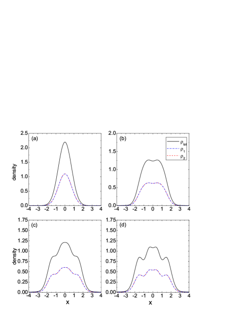
Figure 1: Density distribution of the ground state for $N_{1}=N_{2}=2$. (a) $U_{1}=U_{2}=U_{12}=0.1$; (b) $U_{1}=U_{2}=U_{12}=3.0$; (c) $U_{1}=U_{2}=U_{12}=7.0$; (d) $U_{1}=U_{2}=U_{12}=10.0$.

We first consider the case with the intra- and inter-atomic interactions being same, i.e., $U_{1}=U_{2}=U_{12}$. In Fig. 1, we display the density distributions of two components of Bose gas in a harmonic trap when both components have same particle numbers. As shown in the figures each component of the Bose gas has the same distribution in the whole regime of interaction. In the weak interaction regime, the Bose gas exhibits a Gauss-like distribution, which implies that the many-boson system can be approximately described by a single wave function, i.e., all the bosons condense into the same single state. In the scheme of the mean-field theory, the single wave function is obtained by solving Gross-Pitaevskii equations. In the limit of $U_{\alpha}=0$ ($\alpha=1,2,12$) all atoms occupy the lowest orbital and the ground state takes the form of

$$\psi(x_{1}^{1},\ldots,x_{N_{1}}^{1};x_{1}^{2},\ldots,x_{N_{2}}^{2})=\prod_{i=1}^{N_{1}}\phi_{0}(x_{i}^{1})\prod_{j=1}^{N_{2}}\phi_{0}(x_{j}^{2}),$$

which can be expressed as $|\text{GS}\rangle=(b_{01}^{\dagger})^{N_{1}}(b_{02}^{\dagger})^{N_{2}}|0\rangle$ in our Hilbert space. With the increase of the atomic interaction, the density distribution becomes broader and flatter. When it reaches the strongly interacting regime, four peaks appear at $U_{\alpha}=10$ as shown in the Fig.1d. The emergence of density oscillations is a signal of “fermionization”, i.e., the density profile shows fermion-like distribution Girardeau07 ; Girardeau . In this case, two bosons would avoid to occupying the same orbital and thus the bosons occupy the orbitals one by one similar to the fermions. Therefore the mean-field theory based on the single wave function approximation is not a suitable theory in the strongly interacting limit. To capture the character of density oscillations, more sophistical multi-orbital mean-field theory is required Zoellner ; Zoellner06 ; Cederbaum ; Cederbaum06 .

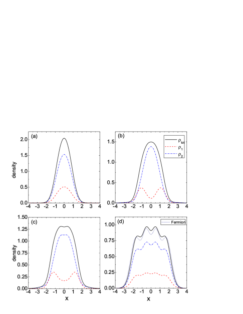
Figure 2: Density distribution of the ground state for $N_{1}=1$ and $N_{2}=3$. (a) $U_{1}=U_{2}=U_{12}=1.0$; (b) $U_{1}=U_{2}=U_{12}=3.0$; (c) $U_{1}=U_{2}=U_{12}=5.0$; (d) $U_{1}=U_{2}=U_{12}=10.0$.

For the imbalanced case with $N_{1}\neq N_{2}$, the total density distribution displays the similar crossover behavior as the case with $N_{1}=N_{2}$. As shown in Fig.2, the halfwidth of the total density distributions becomes larger and larger with the increase of interaction strength, followed by the emergence of an obvious spatial oscillation structure at $U_{\alpha}=10$. What special here is the density distribution for each component is no longer same in the whole interacting regime. In the weakly interacting regime, each component has similar density profile. While in the middle regime, the component of the Bose mixture behaves in different way. At $U_{\alpha}=3$, two obvious peaks are observed for the component with less atoms whereas the total density shows no oscillation. With further increasing the interaction strength to $U_{\alpha}=5$, the total density distribution begins to oscillate with two peaks emerging. When reaching the strongly interacting regime with $U_{\alpha}=10$, four obvious peaks are observed for both components of the Bose mixture. In this limit each component has similar density profile again: the density distribution of the component with $N_{\alpha}$ atoms is ${N_{\alpha}}/{(N_{1}+N_{2})}$ of the total density distribution with $N_{1}+N_{2}$ peaks. As we shall discuss latter, this is consistent with the result in the limit of infinite interaction, where both the total distribution of two species and the respective distribution of them behave like noninteracting spinless fermions.

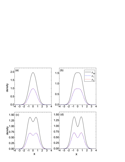
Figure 3: Density distribution of the ground state for $N_{1}=N_{2}=2$ and $U_{1}=U_{2}=0.1$. (a) $U_{12}=0.1$; (b) $U_{12}=3.0$; (c) $U_{12}=5.0$; (d) $U_{12}=10.0$.

In the limit of $U_{\alpha}=\infty$ , we can apply the generalized Bose-Fermi mapping method Girardeau07 ; Deuretzbacher08 to construct the ground state wavefunction of the Bose mixture. According to Girardeau’s argument Girardeau , in the infinite interacting limit the interactions can be replaced by constraints that the many-body wave function vanishes at all collision points Girardeau07 ; Girardeau ; Girardeau02 . It follows that the Girardeau-type ground state wavefunction has the following form

$$\psi(x_{1}^{1},\ldots,x_{N_{1}}^{1};x_{1}^{2},\ldots,x_{N_{2}}^{2})$$ (4)

$$= A(x_{1}^{1},\ldots,x_{N_{1}}^{1},x_{1}^{2},\ldots,x_{N_{2}}^{2})\times$$

$$\psi_{F}(x_{1}^{1},\ldots,x_{N_{1}}^{1};x_{1}^{2},\ldots,x_{N_{2}}^{2})$$

with the antisymmetric function $A(x_{1},x_{2},\ldots,x_{N})=\prod_{1\leq i,j\leq N}\text{sgn}(x_{i}-x_{j})$ and $\psi_{F}(x_{1}^{1},\ldots,x_{N_{1}}^{1};x_{1}^{2},\ldots,x_{N_{2}}^{2})$ is a Slater determinant of $N=N_{1}+N_{2}$ orthonormal orbitals $\phi_{0}(x),\cdots,\phi_{N-1}(x)$ occupied by both components of bosons. Explicitly, we have

$$\psi_{F}(x_{1},\ldots,x_{N})=(N!)^{-\frac{1}{2}}det[\phi_{j}(x_{i})]_{i=1,2,\ldots,N}^{j=0,1,\ldots,N-1}$$

with $x_{1},\ldots,x_{N}$ denoting $x_{1}^{1},\ldots,x_{N_{1}}^{1};x_{1}^{2},\ldots,x_{N_{2}}^{2}$. Now it is straightforward to get

$$\rho_{\alpha}(x)=\frac{N_{\alpha}}{N}\rho_{F}(x)$$ (5)

with $\rho_{F}(x)=\sum_{i=0}^{N-1}\left|\phi_{i}(x)\right|^{2},$ i.e., the densities of both components are proportional to the density of a harmonically trapped TG gas of $N$ bosons which is identical to the density of $N$ free fermions. In Fig. 2d, we compare our numerical result with the exact result in the TG limit. It is clear that the numerical result complies with the exact results very well which implies that the system has entered the strongly interacting regime at this parameter point. Our numerical results provide a clear evidence that the state obtained by Girardeau-type construction Girardeau07 remains to be a good approximation for large but finite repulsion.

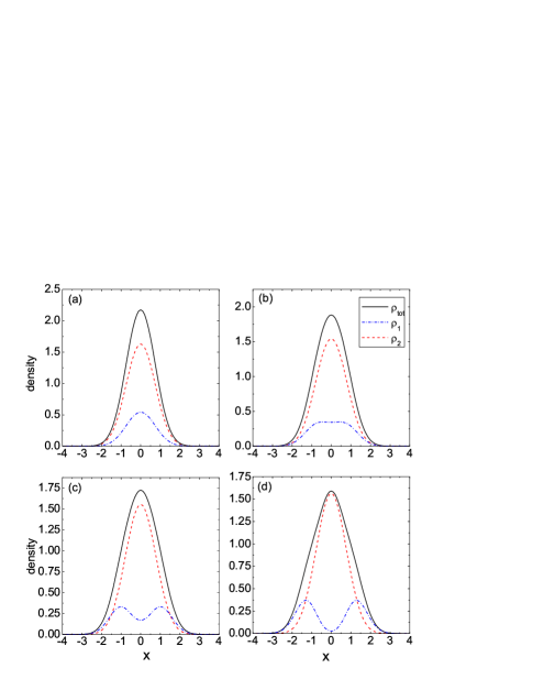
Figure 4: Density distribution of the ground state for $N_{1}=1$, $N_{2}=3$ and $U_{1}=U_{2}=0.1$. (a) $U_{12}=0.1$; (b) $U_{12}=1.0$; (c) $U_{12}=2.0$; (d) $U_{12}=10.0$.

Now we discuss the general case with different intra- and inter-atomic interactions. First we calculate the density distributions for the equal-mixing Bose mixture with equal weak intra-component repulsions. For convenience, we take $U_{1}=U_{2}=0.1$ and $U_{12}\neq U_{1},U_{2}$. Density distributions for different inter-component interactions are shown in Fig. 3. In all the interaction regime, we have $\rho_{1}(x)=\rho_{2}(x)=\frac{1}{2}\rho(x)$. With the increase of $U_{12}$, the density distribution becomes broader. For $U_{12}=5$, two peaks occur. With further increase of inter-component interaction, only two peaks in the density distribution are observed even for $U_{12}=10$. Due to the intra-atomic interaction is weak, each component of atoms may form a condensate. Similar results are found for the system with weak intra-component repulsions even if $U_{1}\neq U_{2}$. The difference from the plot of the case of $U_{1}=U_{2}$ is that the component with stronger intra-atomic interaction distributes in broader regime than that with weaker interaction.

For the case of $N_{1}\neq N_{2}$ with weak intra-atomic interaction $U_{1}=U_{2}=0.1$, density distributions for different inter-component interactions are displayed in the Fig. 4. Similar to the equal-mixing case, the total density distribution becomes flatter with the increase of $U_{12}$. Although two obvious peaks occur for the component with less atoms when $U_{12}=2.0$, no obvious peak is detected in the total density profiles even for $U_{12}=10.0$. When the inter-atomic interaction is strong, the density for the different component has different spacial distribution and gets demixed in order to lower the inter-species interaction energy. As shown in the figures, the component with more atoms stays in the middle of the trap and the component with less atoms stays in the regime away from the middle of the trap.

Finally, we study the change of density distributions versus different inter-component interactions for the Bose mixture with strong intra-atomic interactions. For convenience, we consider the imbalanced case with $N_{1}=3$ and $N_{2}=1$ and we take equal strong intra-component repulsions $U_{1}=U_{2}=10.0$. For the vanishing inter-component interactions, the atoms of two species already lie in the strongly interacting regime and the density distribution for each component gets the Fermi-like feature. The distribution of $\rho_{1}(x)$ displays three peaks and the distribution of $\rho_{2}(x)$ displays one peak. As the inter-atomic interaction increases, the distribution of each component changes continuously as shown in Fig. 5. When $U_{12}=3.0$, the central peak of the first component is suppressed and the density profiles get broader. At $U_{12}=8.0$, four peaks occur for the first component whereas the density for the second component get more flatter accompanying with two peaks discernable. With further increase to $U_{12}=10.0$, both the total density distribution and the distribution of each component show $N_{1}+N_{2}$ peaks and the latter takes on the same distribution normalizing to their own particle numbers $N_{\alpha}$.

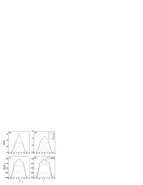
Figure 5: Density distribution of the ground state for $N_{1}=3$, $N_{2}=1$ and $U_{1}=U_{2}=10.0$. (a) $U_{12}=0.0$; (b) $U_{12}=3.0$; (c) $U_{12}=8.0$; (d) $U_{12}=10.0$.

IV Summary

In summary, we have investigated the ground-state properties of two components of Bose gases composed of two hyperfine states of the atoms. With the numerical diagonalization method the density distributions are obtained, which display obviously different properties for different parameters in the system. For the system with equal intra-component and inter-component interactions, the total density distribution shows similar properties to the single-component Bose gases with $N_{1}+N_{2}$ atoms. The evolution from weakly interacting condensate to strongly interacting Tonks gas is shown with the increasing atomic interaction. In the weakly interacting regime the Bose mixture displays Gauss-like distribution whereas in the strongly interacting regime the density distribution gets Fermi-like features. Our numerical result is consistent with the exact result in the infinite limit and thus provides numerical evidence that the Bose mixture can be approximately described by the TG gas even for the system with strong but finite repulsion. We also discuss the general case with different intra-component and inter-component interactions and display the evolution of density distributions from weak to strong inter-component interaction regime for both cases with weak and strong intra-component interactions. Despite the size limitation of the exact diagonalization method used in the present work, our results are no doubt very meaningful because it provides us important insights into the quantum many-body physics beyond various approximate effective-field approaches.

Note added: After finishing the present work Hao08 , we noticed a related work by Zöllner et. al Zoellner08 , in which similar issue was discussed by the multi-orbital self-consistent Hartree method.

- (1) C. J. Myatt et al., Phys. Rev. Lett. 78, 586 (1997).
- (2) M. Erhard, H. Schmaljohann, J. Kronjäger, K. Bongs, and K. Sengstock, Phys. Rev. A 69, 032705 (2004); A. Widera, O. Mandel, M. Greiner, S. Kreim, T. W. Hänsch, and I. Bloch, Phys. Rev. Lett. 92, 160406 (2004).
- (3) T.-L. Ho and V. B. Shenoy, Phys. Rev. Lett. 77, 3276 (1996).
- (4) P. Ao and S. T. Chui, Phys. Rev. A 58, 4836 (1998).
- (5) H. Pu and N. P. Bigelow, Phys. Rev. Lett. 80, 1130 (1998); B. D. Esry, C. H. Greene, J. P. Burke, Jr., and J. L. Bohn, Phys. Rev. Lett. 78, 3594 (1997); E. Timmermans, Phys. Rev. Lett 81, 5718 (1998).
- (6) M. A. Cazalilla and A. F. Ho, Phys. Rev. Lett. 91, 150403 (2003).
- (7) T. Stöferle et al., Phys. Rev. Lett. 92, 130403 (2004).
- (8) B. Paredes, A. Widera, V. Murg, O. Mandel, S. Fölling, I. Cirac, G. V. Shlyapnikov, T. W. Hänsch, and I. Bloch, Nature 429, 277 (2004).
- (9) T. Kinoshita, T. Wenger and D. S. Weiss, Science 305, 1125 (2004).
- (10) M. D. Girardeau, J. Math. Phys. (N.Y.) 1, 516 (1960); Phys. Rev. 139, B500 (1965), Secs. 2, 3, and 6.
- (11) M. Olshanii, Phys. Rev. Lett. 81, 938 (1998).
- (12) T. Bergeman, M. G. Moore, and M. Olshanii, Phys. Rev. Lett. 91, 163201 (2003).
- (13) D. S. Petrov, G. V. Shlyapnikov, and J. T. M. Walraven, Phys. Rev. Lett. 85, 3745 (2000).
- (14) V. Dunjko, V. Lorent and M. Olshanii, Phys. Rev. Lett. 86, 5413 (2001).
- (15) S. Chen and R. Egger, Phys. Rev. A. 68, 063605 (2003).
- (16) Y. Q. Li, S. J. Gu, Z. J. Ying and U. Eckern, Europhys. Lett. 61, 368 (2003).
- (17) E. Eisenberg and E. H. Lieb, Phys. Rev. Lett. 89, 220403 (2002).
- (18) X.-W. Guan, M. T. Batchelor, and M. Takahashi, Phys. Rev. A 76, 043617 (2007).
- (19) J. N. Fuchs, D. M. Gangardt, T. Keilmann, and G. V. Shlyapnikov, Phys. Rev. Lett. 95, 150402 (2005); M. T. Batchelor, M. Bortz, X. W. Guan, and N. Oelkers, J. Stat. Mech. (2006) P03016.
- (20) F. Deuretzbacher, K. Bongs, K. Sengstock, and D. Pfannkuche, Phys. Rev. A 75, 013614 (2007).
- (21) X. Yin, Y. Hao, S. Chen and Y. Zhang, Phys. Rev. A 78, 013604 (2008).
- (22) S. Zöllner, H.-D. Meyer, and P. Schmelcher, Phys. Rev. A 74, 063611 (2006).
- (23) S. Zöllner, H.-D. Meyer, and P. Schmelcher, Phys. Rev. A 74, 053612 (2006).
- (24) O. E. Alon, and L. S. Cederbaum, Phys. Rev. Lett. 95, 140402 (2005).
- (25) A. I. Streltsov, O. E. Alon, and L. S. Cederbaum, Phys. Rev. A 73, 063612 (2006).
- (26) Y. Hao, Y. Zhang, J. Q. Liang and S. Chen, Phys. Rev. A. 73, 063617 (2006).
- (27) Y. Hao, Y. Zhang, and S. Chen, Phys. Rev. A. 76, 063601 (2007).
- (28) M. D. Girardeau and A. Minguzzi, Phys. Rev. Lett. 99, 230402 (2007).
- (29) F. Deuretzbacher, K. Fredenhagen, D. Becker, K. Bongs, K. Sengstock, and D. Pfannkuche , Phys. Rev. Lett. 100, 160405 (2008).
- (30) M. D. Girardeau and E.M. Wright, Laser Phys. 12, 8 (2002).
- (31) Y. Hao and S. Chen, arXiv:0804.1991v1.
- (32) S. Zöllner, H.-D. Meyer, and P. Schmelcher, arXiv:0805.0738.