Alternating dynamic state in intrinsic Josephson-junction stacks self-generated by internal resonance

Abstract

Intrinsic Josephson-junction stacks realized in high-temperature superconductors provide a very attractive base for developing coherent sources of electromagnetic radiation in the terahertz frequency range. A promising way to synchronize phase oscillations in all the junctions is to excite an internal cavity resonance. We demonstrate that this resonance promotes the formation of an alternating coherent state, in which the system spontaneously splits into two subsystems with different phase-oscillation patterns. There is a static phase shift between the oscillations in the two subsystems which changes from $0$ to $2\pi$ in a narrow region near the stack center. The oscillating electric and magnetic fields are almost homogeneous in all the junctions. The formation of this state promotes efficient pumping of the energy into the cavity resonance leading to strong resonance features in the current-voltage dependence.

High-temperature superconductors, such as Bi₂Sr₂CaCu₂O₈ (BSCCO), are composed of two-dimensional superconducting CuO₂-layers coupled via the Josephson effect.KleinerPRL92 The large packing density of these intrinsic junctions makes these compounds very attractive for developing coherent generators of electromagnetic [em] radiation based on the ac Josephson effect. Moreover, a large value of the superconducting gap allows to bring the operation frequency of potential devices into the practically important terahertz range. To develop a powerful source, the major challenge is to synchronize the oscillations of the superconducting phases in a large number of junctions. A very promising route is to excite an internal cavity resonance in finite-size samples (mesas),LutfiSci07 ; KoshBulPRB08 which can entrain oscillations in a very large number of junctions. The frequency of this so-called in-phase Fiske mode is set by the lateral size of the mesa. The experimental demonstration of this mechanism LutfiSci07 has brought the quest for superconducting terahertz sources to a new level.

In general, a mechanism of pumping energy into the cavity mode is a nontrivial issue. Homogeneous phase oscillations at zero magnetic field do not couple to the Fiske modes. Such coupling can be facilitated by introducing an external modulation of the Josephson critical current density.KoshBulPRB08 In this case the amplitudes of the generated standing wave and of the produced radiation are proportional to the strength of modulation.

In this Letter we explore an interesting alternative possibility. Numerically solving the dynamics equation for the Josephson-junction stacks, we found that near the resonance an inhomogeneous synchronized state is formed. In this state, the system spontaneously splits into two subsystems with different phase-oscillation patterns, formally corresponding to fluxon-antifluxon oscillations. Inspired by numerics, we also succeeded to build such solution analytically. The phase oscillations in two subsystems have a static phase shift which has a soliton-shape coordinate dependence, changing from $0$ at one side to $2\pi$ at other side. This change occurs within the narrow region near the center of the stack and the width of this region shrinks when approaching to the resonance. In-spite of the difference in the phase oscillation patterns for the two subsystems, the oscillating electric and magnetic fields are almost identical in all the junctions. The formation of this state strongly enhances coupling to the resonance mode and promotes efficient pumping of energy into the cavity resonance. Such state was also found recently by Lin and Hu.LinHu08

The dynamic equations for the Josephson-junction stacks have been derived in Refs. DynamEqs, and have been used in numerous simulation studies SimulJJ , mostly to study dynamics of the Josephson vortex lattice formed by a magnetic field applied along the layers. We present these equations in the form of coupled time evolution equations for reduced electric and magnetic fields, $e_{n}$ and $h_{n}$, phase differences, $\varphi_{n}$, and the in-plane phase gradients, $k_{n}$, which are very convenient for numerical implementation,

$$\partial e_{n}/\partial\tau =-\nu_{c}e_{n}-g(u)\sin\varphi_{n}+\partial h_{n}/\partial u,$$ (1a)

$$\partial\varphi_{n}/\partial\tau =e_{n},$$ (1b)

$$\partial k_{n}/\partial\tau =-\left(k_{n}+h_{n}-h_{n-1}\right)/\nu_{ab},$$ (1c)

$$h_{n} =\ell^{2}\left(\partial\varphi_{n}/\partial u-k_{n+1}+k_{n}\right).$$ (1d)

The units and definitions of parameters are summarized in Table 1 and its caption. These reduced equations depend on three parameters, $\nu_{c}\!=\!4\pi\sigma_{c}/(\varepsilon_{c}\omega_{p})$, $\nu_{ab}\!=\!4\pi\sigma_{ab}/(\varepsilon_{c}\omega_{p}\gamma^{2})$, and $\ell\!=\!\lambda/s$, where $\sigma_{c}$ and $\sigma_{ab}$ are components of the quasiparticle conductivity. We neglected the in-plane displacement current which would give a term $\sim\partial^{2}k_{n}/\partial\tau^{2}$, because relevant frequencies are much smaller than the in-plane plasma frequency.

We simulated a stack containing $N$ junctions ($1\!\leq\!n\!\leq N$), having a width of $L\lambda_{J}$ ($0\!<\!u\!<\!L$), and assuming that the dynamic state is homogeneous in the third direction. We study the voltage range corresponding to the Josephson frequencies close to the lowest in-phase resonance frequency $\omega_{1}=\pi\ell/L$. The function $g(u)\!=\!1\!-\!2r(u\!-\!L/2)/L$ in Eq. (1a) describes a linear modulation of the Josephson current density, which provides coupling to this mode for c-axis homogeneous oscillations.KoshBulPRB08 Our purpose is to probe the qualitative structure of the resonance states and, for simplicity, we assume nonradiative boundary conditions at the edges, $k_{n}=0$, $\partial\varphi_{n}/\partial u=\mp I/2\ell^{2}$, for $u=0,L$, where $I$ is the transport current flowing through the stack, and metallic contacts at the top and the bottom, $k_{0}=k_{N+1}=0$.

Table 1. Units of physical variables. Here $\omega_{p}$ is plasma frequency, $\lambda_{J}$ is the Josephson length, $s$ is the interlayer period, $\lambda$ is the in-plane London penetration depth, $\gamma$ is the anisotropy factor, and $j_{J}$ is the Josephson current density. Variable time, $\tau$ coordinate, $u$ phase gradient, $k_{n}$ electric field, $e_{n}$ magnetic field, $h_{n}$ current density, $j$ Unit $1/\omega_{p}$ $\lambda_{J}$ $1/\lambda_{J}$ $\Phi_{0}\omega_{p}/(2\pi cs)$ $\Phi_{0}/(2\pi\gamma\lambda^{2})$ $j_{J}$

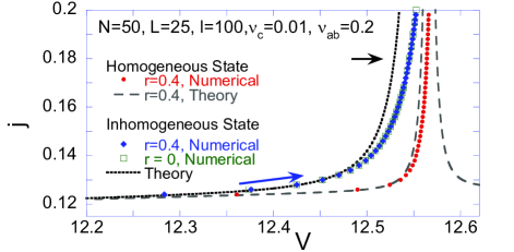
Figure 1: Simulated and theoretical CVDs in the vicinity of the resonance voltage for different states with $V\!=\!\langle e_{n}\rangle\!=\!\omega$. Small circles show the dependence obtained for $r=0.4$ and c-axis homogeneous initial state, which remains homogeneous with increasing current. The theoretical CVD for this stateKoshBulPRB08 is shown by grey dashed line. Small filled diamonds show the CVD for $r=0.4$ and inhomogeneous state, which was self-generated when small $n$-dependent perturbation was added to the phase in the beginning of run for each current value. The open squares represents the CVD for $r\!=\!0$, when the inhomogeneous state has been used as the initial state at starting current. The inhomogeneous state is not sensitive to modulation. Dotted black line shows the theoretical curve for the inhomogeneous state based on Eqs. (6) and (13).

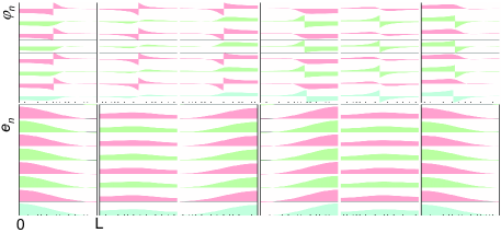
Figure 2: Snapshots of the phase and electric field configurations in the 8 bottom junctions for the same parameters as in Fig. 1 and $j=0.18$ marked by the arrow.Animations The phases are reduced to the interval $[-\pi,\pi]$, so that jumps formally correspond to centers of the Josephson vortices. The dynamic state corresponds to alternating nucleation, motion and annihilation of vortices in the even junctions and antivortices in the odd junctions. Vortex velocities near the edges much larger than near the center. In between $3^{\mathrm{r}d}$ and $4^{\mathrm{t}h}$ configurations jumplike annihilation of fluxons and nucleation of antifluxons take place at the right side. The lower plots show that the electric field is homogeneous in all junctions and has space/time dependence corresponding to the fundamental mode. The annihilation/nucleation events correspond to maxima of electric fields at the edges.

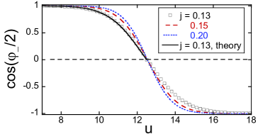
Figure 3: Cosine of half static phase shift between phases in two subsystems at different currents. One can see that the phase shift has shape of soliton and it narrows with approaching to the resonance. Solid line shows theoretical curve based on Eq. (12) and using Eqs. (9), (10), and (13) for $j=0.13$. This function determines the coupling of the homogeneous Josephson oscillations to the internal resonance mode.

Figure 1 shows the current-voltage dependences (CVDs) obtained for representative system parameters listed in the plot and for two values of the modulation parameter $r=0$ and $0.4$. The dependences have been obtained with increasing current. We observe a strong resonance enhancement of the current due to the excitation of the internal cavity resonance. As our simulations do not take into account thermal noise, the emerging state is sensitive to the initial configuration. If we start with a c-axis homogeneous state it remains homogeneous up to certain current. In this case the resonance is excited due to the finite modulation and it is well described by theory developed in Ref. KoshBulPRB08, . However, if we add a small $n$-dependent perturbation to the phase at the start of every current run, the homogeneous state blows up and the system organizes itself into a coherent inhomogeneous state. We also studied a system without modulation using an inhomogeneous state as initial state and found that the corresponding CVD is practically undistinguishable from the one for the modulated system. Therefore, the modulation of the critical current density triggers the transition to the inhomogeneous state but once being formed, this state is not sensitive to the modulation any more.

To understand the nature of the inhomogeneous state, we show in Fig. 2 the time evolution of the phase and electric field for the 8 bottom junctions for $j=0.18$. We see that the system splits into two alternating subsystems with different phase dynamics, corresponding to fluxon/antifluxon oscillations. In the first half period vortices nucleate at the left side in even junctions, rapidly move to the center, then, after slow motion near the center, rapidly annihilate at the right side. Immediately after that, in the second half period, antivortices nucleate at the right side in the odd junctions, move to the left in a similar way, and annihilate at the left side. In spite of the difference in the phase dynamics between the two subsystems, the electric and magnetic fields are almost identical in all junctions. For the electric field, this can be seen from the lower plots of Fig. 2. The dominating contribution to the oscillating electric field is given by the fundamental cavity mode, $e_{n}\propto\cos(\pi u/L)$.

The homogeneity of the electric field implies that there is a static phase shift between the phase oscillations in the two subsystems. Figure 3 shows the cosine of half of this phase shift at different currents. One can see that the phase shift has the shape of a soliton and its width shrinks with increasing current.

To study the dynamic state analytically, we assume that the system is split into two alternating subsystems, $\varphi_{2m+1}=\varphi_{1}$, $\varphi_{2m}=\varphi_{2}$.footnote1122 Introducing new variables, $\varphi_{+}=(\varphi_{1}+\varphi_{2})/2$ and $\varphi_{-}=\varphi_{2}-\varphi_{1}$, and excluding other variables, we derive from Eqs. (1) for $\ell\gg 1$

$$\frac{\partial^{2}\varphi_{+}}{\partial\tau^{2}} +\nu_{c}\frac{\partial\varphi_{+}}{\partial\tau}-\ell^{2}\frac{\partial^{2}\varphi_{+}}{\partial u^{2}}=-\sin\varphi_{+}\cos\left(\varphi_{-}/2\right),$$ (2a)

$$\frac{\partial^{2}\varphi_{-}}{\partial\tau^{2}} +\nu_{c}\frac{\partial\varphi_{-}}{\partial\tau}-\frac{1}{4}\left(1+\nu_{ab}\frac{\partial}{\partial\tau}\right)\frac{\partial^{2}\varphi_{-}}{\partial u^{2}}$$

$$=-2\sin\left(\varphi_{-}/2\right)\cos\varphi_{+}.$$ (2b)

We now obtain a self-consistent approximate solution of these equations for the dynamic state when the Josephson frequency, $\omega=\langle e_{n}\rangle$, is close to the resonance frequency, $\omega_{1}=\pi\ell/L$. We will show that $\varphi_{-}$ is almost static. In this case the equation for $\varphi_{+}$ coincides with the phase equation for the Josephson junction with modulated Josephson current density KoshBulPRB08 with modulation function $g(u)\!=\!\cos\left(\varphi_{-}/2\right)$, see Fig. 3. Near the resonance frequency, we make the mode projection for $\varphi_{+}$,

$$\varphi_{+}(u,\tau)=\omega\tau+\operatorname{Re}[\psi\exp(-i\omega\tau)]\cos(\pi u/L),$$ (3)

and, assuming $|\psi|\ll 1$, we obtain

$$\psi =\frac{ig_{-}}{\omega^{2}-\omega_{1}^{2}+i\nu_{c}\omega},$$ (4)

$$\text{with }g_{-} =\frac{2}{L}\int_{0}^{L}\cos(\pi u/L)\cos\left(\varphi_{-}/2\right)du$$ (5)

being the coupling parameter. This solution determines the CVD, which takes into account resonance enhancement of the Josephson currentKoshBulPRB08 ,

$$j(V)\approx\nu_{c}V+\frac{g_{-}^{2}\nu_{c}V/4}{\left(\omega_{1}^{2}-V^{2}\right)^{2}+\left(\nu_{c}V\right)^{2}}.$$ (6)

To evaluate $\varphi_{-}(u,\tau)$, we split it into static and dynamic parts, $\varphi_{-}(u,\tau)=\bar{\varphi}_{-}(u)+\tilde{\varphi}_{-}(u,\tau)$. Further analysis shows that $\tilde{\varphi}_{-}(u,\tau)\ll 1$. The static part is determined by

$$d^{2}\varphi_{-}/du^{2}-8C_{+}(u)\sin(\varphi_{-}/2)=0$$ (7)

with $C_{+}(u)\!\equiv\!\left\langle\cos\varphi_{+}\right\rangle$. Using Eqs. (3) and (4), we obtain

$$C_{+}(u) \approx C_{1}\cos(\pi u/L),$$ (8)

$$\text{with }C_{1} =-\frac{\operatorname{Im}[\psi]}{2}=-\frac{g_{-}}{2}\frac{\omega^{2}-\omega_{1}^{2}}{\left(\omega^{2}-\omega_{1}^{2}\right)^{2}+\left(\nu_{c}\omega\right)^{2}}.$$ (9)

Consider the region near the midpoint, $u=L/2$, where the static cosine can be approximated by the linear function $C_{+}(u)\approx C_{1}(\pi/L)(L/2-u)$. Using the substitution

$$v=(u-L/2)/l_{s}\text{ with }l_{s}=\left[L/\left(8\pi C_{1}\right)\right]^{1/3},$$ (10)

we can reduce Eq. (7) near the midpoint to the dimensionless form

$$d^{2}\varphi_{-}/dv^{2}+v\sin(\varphi_{-}/2)=0.$$ (11)

This equation allows for soliton solution in which $\varphi_{-}$ changes from $0$ to $2\pi$ within $|v|\sim 1$, corresponding to $|u-L/2|\sim l_{s}$. In the case $l_{s}\ll L$  the linear expansion for $C_{+}(u)$ is valid in the soliton core and Eq. (11) determines its shape with a very good accuracy. In the range $\omega_{1}^{2}\!-\!\omega^{2}\gg\nu_{c}\omega$ the condition $l_{s}\!\ll\!L$ is equivalent to $\omega_{1}^{4}(1\!-\!(\omega/\omega_{1})^{2})\!\ll\!4\pi^{2}\ell^{2}$. As typically $\ell\approx 150$, this condition is always satisfied in the interesting frequency range. The soliton solution has the symmetry $\varphi_{-}(v)=2\pi-\varphi_{-}(-v)$. Numerically solving Eq. (11), we can interpolate the solution as

$$\varphi_{-}(v)\approx\pi\exp\left\{-(\sqrt{2}/3)\left[\left(|v|\!+\!C_{v}\right)^{3/2}\!-C_{v}^{3/2}\right]\right\}$$ (12)

for $v\!<\!0$ with $C_{v}\approx 0.5129$.

To evaluate the coupling constant (5), we note that $\cos\left(\varphi_{-}/2\right)$ changes from $1$ to $-1$ within a narrow region near the midpoint, $|u\!-\!L/2|\!\sim\!l_{s}$ meaning that, up to terms $\sim\!\left(l_{s}/L\right)^{2}$, $\cos(\varphi_{-}/2)$ can be approximated by $\mathrm{sign}(L/2\!-\!u)$ which gives $g_{-}\!\approx\!4/\pi$. Surprisingly, this self-generated steplike modulation provides the maximum possible coupling to the resonance mode. Correction to $g_{-}$ due to the finite soliton width can be evaluated as

$$\delta g_{-}\!=\!\frac{4}{L}\int_{0}^{L/2}\!\cos\!\left(\frac{\pi u}{L}\right)\left(\cos\!\frac{\varphi_{-}}{2}-\!1\right)\!du\!\approx\!-0.464\frac{4\pi l_{s}^{2}}{L^{2}}.$$

Adding this correction and using Eqs. (10) and (9), the total coupling parameter can be written as

$$g_{-}\approx\frac{4}{\pi}\left\{1-1.817\left[\frac{\left(\omega_{1}^{2}-\omega^{2}\right)L^{2}}{\left(\omega^{2}-\omega_{1}^{2}\right)^{2}+\left(\nu_{c}\omega\right)^{2}}\right]^{-2/3}\right\}$$ (13)

As $g_{-}\sim 1$, the used linear approximation $|\psi|\ll 1$ is valid only at $|\omega^{2}-\omega_{1}^{2}|>1$.

To evaluate the time-dependent part of $\varphi_{-}$, we represent it in the complex form, $\tilde{\varphi}_{-}(\tau,u)=\operatorname{Re}\left[\tilde{\varphi}_{-}(u)\exp(-i\omega\tau)\right]$, and separating the time-dependent part of Eq. (2b), we derive the equation for the complex amplitude

$$\left(\omega^{2}+i\nu_{c}\omega\right)\tilde{\varphi}_{-}+\frac{1\!-\!i\nu_{ab}\omega}{4}\frac{\partial^{2}\tilde{\varphi}_{-}}{\partial u^{2}}=2\sin\frac{\bar{\varphi}_{-}}{2}$$

In the range $\omega\!\gg\!1$, we estimate $\tilde{\varphi}_{-}\!\approx\!2\sin\left(\bar{\varphi}_{-}/2\right)/\omega^{2}\!\ll\!1$. The small amplitude of $\tilde{\varphi}_{-}(\tau,u)$ justifies usage of the static approximation for $\varphi_{-}$ in the equation for $\varphi_{+}$.

To compare analytical results with numerics, we show in Fig. 3 the theoretical result for $\cos(\varphi_{-}/2)$ at $j\!=\!0.13$ based on Eq. (12). It accurately describes the numerical data. The theoretical prediction for the CVD based on Eqs. (6) and (13) is shown in Fig. 1. The linear approximation describes well the numerical data for voltages not too close to the resonance. Due to the enhancement of nonlinearities in the vicinity of the resonance, the analytical result overestimates the current increase.

The found state looks similar to the fluxon-antifluxon oscillations in a single junction.FultonDynesSSC73 These oscillations appear as a result of a parametric instability of the homogeneous oscillations CostabilePRB87 and lead to so-called zero-field steps in the CVDs.Chen71 The Josephson frequency of such step is twice the frequency of the involved resonance. In spite of the apparent similarity, there are essential qualitative differences. In the case of a stack, the frequency coincides with the resonance frequency. The dynamic configurations are also very different. In the case of a single junction, a well-developed fluxon nucleates at one side, moves with Swihart velocity to the other side, converts to the antifluxon there, which then moves back again with constant velocity FultonDynesSSC73 . In our case, there is a region statically located near the center where rapid phase change $\pm\pi$ is localized, corresponding to $2\pi$ phase change of $\phi_{-}$. As a consequence, the centers of fluxons and antifluxons, formally defined as points where the phases are commensurate with $\pm\pi$, spend most time near the center and very rapidly jump to and from the edges, see Fig. 2. Moreover, the fluxon interpretation of our oscillations is somewhat artificial, as there are no well-defined localized soliton excitations moving across the junctions.

The alternating state is a plausible candidate for the coherent state responsible for resonant terahertz emission observed in Ref. LutfiSci07, . Even though we did not use boundary conditions accounting for the radiation, it is clear that the generation of such a state would lead to powerful emission. In fact, the radiation does not influence much the structure of the internal states for short mesas, $N\lesssim 100$, and em emission can be approximately computed from the oscillating electric fields at the edges.KoshBulPRB08 For taller mesas, the radiation may contribute to the resonance damping but we do not expect that it will destroy the coherent state. The experimental resonance features in the CVDs are much weaker then the theoretical ones. The possible mechanisms reducing the amplitude of the resonance include noise, c-axis inhomogeneities, and additional damping channels not taken into account by the theoretical model.

The author would like to thank U. Welp, L. Bulaevskii, K. Gray, M. Tachiki, and X. Hu for useful discussions. This work was supported by the U.​ S. DOE, Office of Science, under contract # DE-AC02-06CH11357.

References

- (1) R. Kleiner, et al., Phys. Rev. Lett. 68, 2394 (1992); R. Kleiner and P. Müller, Phys.Rev. B 49, 1327 (1994).
- (2) L. Ozyuzer, et al., Science 318, 1291 (2007); K. Kadowaki, et al., unpublished.
- (3) A. E. Koshelev and L. N. Bulaevskii, Phys. Rev. B, 77, 014530, (2008).
- (4) Shizeng Lin and Xiao Hu, arXiv:0803.4244, unpublished.
- (5) S. Sakai, P. Bodin, and N. F. Pedersen, J. Appl. Phys. B 73, 2411 (1993); L. N. Bulaevskii, et al., Phys. Rev. B 53, 14 601 (1996); S. N. Artemenko and S. V. Remizov, JETP Lett. 66, 853 (1997).
- (6) M. Machida, et al., Phys. Rev. Lett., 83, 4618 (1999); R. Kleiner, et al., Phys. Rev. B, 62, 4086 (2000); S. Madsen and N. F. Pedersen, Phys. Rev. B, 72, 134523 (2005); M. Tachiki, et al., Phys. Rev. B, 71, 134515 (2005); B. Y. Zhu, et al., Phys. Rev. B, 72, 174514 (2005); Sh. Lin, et al., Phys. Rev. B, 77, 014507 (2008).
- (7) This alternating solution with the periodicity 1-2-1-2- is not the only possible state. The solution with the periodicity 1-1-2-2-1-1- also can be built in a similar way.
- (8) Animations of these configurations can be seen at http://mti.msd.anl.gov/homepages/koshelev/projects/AlternState.
- (9) T. A. Fulton and R. C. Dynes, Sol. St. Comm., 12, 57 (1973); P. S. Lomdahl, O. H. Soerensen, and P. L. Christiansen, Phys. Rev. B, 25, 5737 (1982).
- (10) G. Costabile, S. Pagano, and R. D. Parmentier, Phys. Rev. B, 36, 5225 (1987).
- (11) J. T. Chen, T. F. Finnegan, and D. N. Langenberg, Physica, 55, 413 (1971).