The classical hydrodynamics of the Calogero-Sutherland model

Abstract

We explore the classical version of the mapping, due to Abanov and Wiegmann, of Calogero-Sutherland hydrodynamics onto the Benjamin-Ono equation “on the double.” We illustrate the mapping by constructing the soliton solutions to the hydrodynamic equations, and show how certain subtleties arise from the need to include corrections to the naïve replacement of singular sums by principal-part integrals.

I Introduction

The Calogero-Sutherland family of models [1, 2] consist of point particles moving on a line or circle and interacting with a repulsive inverse-square potential. Both the classical and quantum versions are completely integrable, and are the subject of an extensive literature [3]. The models have application to one-dimensional electron systems [4], and to the two-dimensional quantum Hall effect [5].

It is possible to consider a hydrodynamic limit of the Calogero-Sutherland models in which the distribution and velocity of the particles are described by continuous fields $\rho(x)$ and $v(x)$ respectively. The equations of motion of these fields possess solitary wave solutions, and also periodic solutions that interpolate between small amplitude sound waves and large amplitude trains of solitary waves [6, 7]. The quantum version of the hydrodynamics provides an extension of the usual theory of bosonization of relativistic (i.e. linear dispersion) electron systems to systems where band-curvature effects become important [8]. Because of the singular nature of the Calogero-Sutherland interaction, the hydrodynamic limit is rather more subtle than one might expect. Considerable insight into this limit has been provided by Abanov and Wiegmann who have shown [9] that it is equivalent to a “doubled” version of Benjamin-Ono dynamics [10, 11]. The Benjamin-Ono equation, a member of an infinite hierarchy of integrable partial differential equations, was originally introduced to describe waves in stratified fluids. The connection has lead to a number of novel predictions for the evolution of one-dimensional electron gasses [12].

In this paper we will apply the tools of [9] to recover the classical soliton solutions found in [6, 7] and, in doing so, illustrate the structure of the Calogero-Sutherland $\leftrightarrow$ Benjamin-Ono mapping. A secondary aim is to compare the origin of the hydrodynamic-limit subtleties in the classical model with their origin in the quantum system. In the quantized model they arise because of the need to convert operators that are hermitian with respect to one of the two natural inner products on the Calogero-Sutherland Hilbert space into operators that are hermitian with respect to the other [13]. In the classical model the subtleties arise because we need to include corrections to the naïve limit of singular sums.

In section II, we review the connection between the Calogo-Sutherland and Benjamin-Ono equations of motion. In section III we consider an appealing, but overly naïve, version of the hydrodynamic limit and reveal its failings. In section IV we illustrate how these shortcomings are eliminated by including the first non-trivial order in an asymptotic expansion for the velocity field. In section V we consider the general mapping. An appendix contains proofs of some results used in the main text.

II Calogero-Sutherland from the Benjamin-Ono pole ansatz

The classical Benjamin-Ono equation [10, 11] is the nonlinear and and non-local partial differential equation

$$\dot{u}+u\,\partial_{x}u=\textstyle{1\over 2}\lambda(\partial^{2}_{xx}u)_{H},$$ (1)

where $f_{H}$ denotes the Hilbert transform of $f$:

$$f_{H}(x)\,\stackrel{{\scriptstyle\rm def}}{{=}}\,{\rm P\over\pi}\int_{-\infty}^{\infty}{1\over x-\xi}f(\xi)\,d\xi.$$ (2)

If we introduce a Poisson bracket

$$\{u(x),u(x^{\prime})\}=2\lambda\pi\,\partial_{x}\delta(x-x^{\prime}),$$ (3)

and Hamiltonian

$$H_{\rm BO}={1\over 2\lambda\pi}\int_{-\infty}^{\infty}\left\{{1\over 6}u^{3}-{\lambda\over 4}u(u_{x})_{H}\right\}dx,$$ (4)

then (1) can be written as $\dot{u}(x,t)=\{H_{\rm BO},u(x,t)\}$. This Hamiltonian system possesses infinitely many Poisson-commuting integrals of motion [14].

Following [15], we seek solutions of (1) as a sum of poles

$$u(x,t)=\sum_{j=1}^{N}{i\lambda\over x-a_{j}(t)}-\sum_{j=1}^{M}{i\lambda\over x-b_{j}(t)}.$$ (5)

The poles at $a_{j}(t)$, $j=1,\ldots,N$, lie below the real axis while the poles at $b_{j}(t)$, $j=1,\dots,M$, lie above it. In [15], the numbers of $a_{j}$ and $b_{j}$ poles were set equal and $b_{j}(t)=a_{j}^{*}(t)$. These conditions were imposed to ensure that $u(x,t)$ was real. We will not make these assumptions, so our field $u(x,t)$ is not necessarily real-valued.

We insert the ansatz (5) into (1) and use

$$\left({1\over x-a}\right)_{H}=\cases{\displaystyle{{-i\over x-a}},&${\rm Im\,}a<0$\vskip 3.0pt plus 1.0pt minus 1.0pt\cr\displaystyle{{+i\over x-a}},&${\rm Im\,}a>0$}$$ (6)

to find

$$\left\{\sum_{k=1}^{N}{i\lambda\dot{a}_{k}\over(x-a_{k})^{2}}-\sum_{k=1}^{M}{i\lambda\dot{b}_{k}\over(x-b_{k})^{2}}\right\}-\left\{\sum_{j=1}^{N}{i\lambda\over x-a_{j}}-\sum_{j=1}^{M}{i\lambda\over x-b_{j}}\right\}\left\{\sum_{k=1}^{N}{i\lambda\over(x-a_{k})^{2}}-\sum_{k=1}^{M}{i\lambda\over(x-b_{k})^{2}}\right\}$$

$$\qquad\qquad-\lambda\left\{\sum_{j=1}^{N}{\lambda\over(x-a_{j})^{3}}+\sum_{j=1}^{M}{\lambda\over(x-b_{j})^{3}}\right\}=0.$$ (7)

All terms with $1/(x-a_{i})^{3}$ and $1/(x-b_{i})^{3}$ cancel directly. The remaining terms can be simplified by exploiting the identity

$${1\over(x-c_{1})}{1\over(x-c_{2})^{2}}+{1\over(x-c_{2})}{1\over(x-c_{1})^{2}}={1\over(c_{2}-c_{1})}{1\over(x-c_{2})^{2}}+{1\over(c_{1}-c_{2})}{1\over(x-c_{1})^{2}},$$ (8)

to rearrange them as a sum of $1/(x-a_{i})^{2}$’s and $1/(x-b_{i})^{2}$’s with $x$-independent coeffcients. Now the set of $1/(x-a_{i})^{2}$’s and $1/(x-b_{i})^{2}$’s is linearly independent, and the vanishing of their individual coefficients requires

$$i\dot{a}_{j} = \sum_{k;\,k\neq j}{\lambda\over(a_{k}-a_{j})}-\sum_{k=1}^{M}{\lambda\over(b_{k}-a_{j})},\$$ (9)

$$i\dot{b}_{j} = \sum_{k;\,k\neq j}{\lambda\over(b_{j}-b_{k})}-\sum_{k=1}^{N}{\lambda\over(b_{j}-a_{k})}.$$ (10)

We have found $N+M$ evolution equations for $N+M$ variables, and so the pole ansatz is internally consistent.

We now compute $\ddot{a}_{j}$ by differentiating (9), and then using equations (9), (10) to eliminate the $\dot{a}_{i}$ and $\dot{b}_{i}$’s. After some labour involving repeated use of (8) we find that

$$\ddot{a}_{j}=\sum_{k;\,k\neq j}{2\lambda^{2}\over(a_{j}-a_{k})^{3}}.$$ (11)

Remarkably, the $b_{j}(t)$ do not appear. The only role of the $b_{j}$’s in the $a_{i}$-pole dynamics is that the complex parameters $b_{j}(0)$ determine the (complex) initial velocities $\dot{a}_{i}(0)$ of the $a_{i}(t)$-poles. Once these initial conditions are established, the $a_{i}$ poles evolve autonomously according to (11).

The $N$ equations (11) are a complex version of the Calogero model equations of motion. As for the real-$a_{i}$ case, they can be derived from the many-body Lagrangian

$$L_{\rm Calogero}={1\over 2}\sum_{i=1}^{N}\dot{a}_{i}^{2}-{1\over 2}\sum_{i,j;\,i\neq j}{\lambda^{2}\over(a_{i}-a_{j})^{2}}.$$ (12)

We may site our initial poles so that if we place a pole at $z$, then we also place one at $z+2\pi n$ for any integer $n$. The resulting $2\pi$ periodicity will be preserved by the subsequent evolution. The sums

$$\lim_{M\to\infty}\left\{\sum_{n=-M}^{M}{1\over z+2\pi n}\right\} = {1\over 2}\cot\left({z\over 2}\right),$$ (13)

$$\sum_{n=-\infty}^{\infty}{1\over(z+2\pi n)^{2}} = {1\over 4}{\rm cosec}^{2}\left({z\over 2}\right),$$ (14)

then allow us to write the evolution equations in the form

$$i\dot{a}_{j} = \sum_{k;\,k\neq j}{\lambda\over 2}\cot\left({a_{k}-a_{j}\over 2}\right)-\sum_{k=1}^{M}{\lambda\over 2}\cot\left({b_{k}-a_{j}\over 2}\right),\$$ (15)

$$i\dot{b}_{j} = \sum_{k;\,k\neq j}{\lambda\over 2}\cot\left({b_{j}-b_{k}\over 2}\right)-\sum_{k=1}^{N}{\lambda\over 2}\cot\left({b_{j}-a_{k}\over 2}\right),$$ (16)

and

$$\ddot{a}_{j}=-{\partial\over\partial a_{j}}\left\{{1\over 4}\sum_{k;\,k\neq j}{\lambda^{2}\over{\rm sin}^{2}(a_{j}-a_{k})/2}\right\}.$$ (17)

If we regard the $a_{i}$ as angles, then (17) is the equation of motion arising from the Sutherland-model Lagrangian

$$L_{\rm Sutherland}={1\over 2}\sum_{i=1}^{N}\dot{a}_{i}^{2}-{1\over 8}\sum_{i,j;\,i\neq j}{\lambda^{2}\over{\rm sin}^{2}(a_{i}-a_{j})/{2}}$$ (18)

for particles on a circle.

The authors of [15] made $b_{i}=a_{i}^{*}$, as they wished $u(x,t)$ to be real. Being interested primarily in Calogero-Sutherland models, we instead desire that the $a_{i}(t)$ be real. To arrange for this, we modify the definition of the Hilbert transform (2) appearing in (1). Following Abanov and Wiegmann [9] we define the $\Gamma$-contour Hilbert transform of $u$ to be

$$u_{\Gamma}(z)\,\stackrel{{\scriptstyle\rm def}}{{=}}\,{\rm P\over\pi}\oint_{\Gamma}{1\over z-\xi}f(\xi)\,d\xi,$$ (19)

where $\Gamma$ is a simple closed contour on which $z$ lies. All that was needed to establish the $a$-pole autonomy was that the $1/(x-a_{i})$’s and $1/(x-b_{i})$’s be eigenfunctions of the Hilbert transform with eigenvalues of opposite sign. Now if we take $\Gamma$ to encircle the real axis in a clockwise sense (as shown in Figure 1) then, for $z$ on the contour,

$$\left({1\over z-a_{i}}\right)_{\Gamma} = {-i\over z-a_{i}},$$

$$\left({1\over z-b_{i}}\right)_{\Gamma} = {+i\over z-b_{i}},$$ (20)

when the $a_{i}$ poles lie within $\Gamma$ and the $b_{i}$ poles lie outside. We can therefore let the $a_{i}(0)$ lie on the real axis and distribute the $b$-poles in the remainder of the complex plane in such a manner that the initial $\dot{a}_{i}$’s are real. Once the intitial $a_{i}$’s and $\dot{a}_{i}$’s are real, the Calogero evolution ensures that the $a_{i}(t)$ remain on the real axis. Thus, a complex Benjamin-Ono field $u(z,t)$ obeying

$$\dot{u}+u\,\partial_{z}u=\textstyle{1\over 2}\lambda(\partial^{2}_{zz}u)_{\Gamma}$$ (21)

on $\Gamma$ can provide real-axis Calogero-Sutherland dynamics.

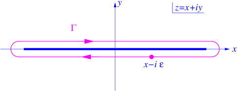
Figure 1: The contour $\Gamma$ surrounds the part of the real axis on which the $a_{i}$ poles are found.

III Shepherd poles and Calogero density-wave solitons

In this section we will apply the pole ansatz to obtain solitary wave solutions to the hydrodynamic limit of the real-axis Calogero equation. In this limit we let the number $N$ of Calogero particles become infinite, while keeping their density finite. We then replace the individual $a_{i}(t)$ by a smooth particle-number density $\rho(x,t)$, and the individual velocities $\dot{a}_{i}(t)$ by a smooth velocity field $v(x)$. We assume that $\rho$ and $v$ vary slowly on the scale of the inter-particle spacing. We are now naturally tempted to approximate the discrete $a$-pole sums in the evolution equations

$$i\dot{a}_{j} = \sum_{k;\,k\neq j}{\lambda\over a_{k}-a_{j}}-\sum_{k}{\lambda\over b_{k}-a_{j}},$$

$$i\dot{b}_{j} = \sum_{k;\,k\neq j}{\lambda\over b_{j}-b_{k}}-\sum_{k}{\lambda\over b_{j}-a_{k}},$$ (22)

by integrals to get

$$i\dot{a}(x,t) = {\rm P\!\!}\int_{-\infty}^{\infty}{\lambda\over\xi-x}\rho(\xi,t)\,d\xi-\sum_{k}{\lambda\over b_{k}-x},$$

$$i\dot{b}_{j}(t) = \sum_{k;\,k\neq j}{\lambda\over b_{j}-b_{k}}-\int_{-\infty}^{\infty}{\lambda\over b_{j}-\xi}\rho(\xi,t)\,d\xi.$$ (23)

Here, $\dot{a}(x,t)\equiv v(x,t)$ is the velocity of the pole at $x$. We begin by exploring the consequences of this approximation to the discrete sum. We will see that it is not quite consistent, and a small but significant correction is needed.

Consider an initial density fluctuation

$$\rho(x,0)=\rho_{0}+\rho_{1}(x),\quad\hbox{where}\quad\rho_{1}(x)=\left({A\over\pi}\right){1\over x^{2}+A^{2}}.$$ (24)

Because

$$\int_{-\infty}^{\infty}\left({A\over\pi}\right){1\over\xi^{2}+A^{2}}\,d\xi=1,$$ (25)

the Lorentzian distribution $\rho_{1}(x)$ corresponds to a local excess of one particle near $x=0$.

The contribution

$${\rm P}\int_{-\infty}^{\infty}{\lambda\over\xi-x}\left({A\over\pi}\right){1\over\xi^{2}+A^{2}}\,d\xi=-{\lambda x\over x^{2}+A^{2}},\quad({\rm Im\,}x=0)$$ (26)

of the density fluctuation to $i\dot{a}$ is real, and so tends to push $a(x)$ off the real axis. Its effect can be countered, however, by placing a solitary $b$-pole at at $b=iA$. We then have

$$i\dot{a}(x,0) = -{\lambda x\over x^{2}+A^{2}}+{\lambda\over x-iA}$$ (27)

$$= -{\lambda x\over x^{2}+A^{2}}+{\lambda(x+iA)\over x^{2}+A^{2}}$$

$$= {iA\lambda\over x^{2}+A^{2}},$$

and the $a$ poles have a purely real initial velocity

$$v(x,0){=}\dot{a}(x,0)={A\lambda\over x^{2}+A^{2}}.$$ (28)

They therefore stay on the real axis.

The motion of the $b=iA$ pole is obtained from

$$i\dot{b} = -\int_{-\infty}^{\infty}{\lambda\over b-\xi}\left({A\over\pi}\right){1\over\xi^{2}+A^{2}}\,d\xi-\int_{-\infty}^{\infty}{\lambda\rho_{0}\over b-\xi}\,d\xi$$ (29)

$$= -{\lambda\over b+iA}+i\lambda\pi\rho_{0}$$

$$= {i\lambda\over 2A}+i\lambda\pi\rho_{0}.$$

Thus, the $b$-pole velocity

$$\dot{b}={\lambda\over 2A}+\lambda\pi\rho_{0}$$ (30)

is also purely real. Since we know that the $a$ poles stay on the real axis, it must be that the $a$-pole density profile keeps abreast of the $b$ pole as it moves parallel to the real axis. A constant-shape solitary wave of density

$$\rho(x,t)=\rho_{0}+\left({A\over\pi}\right){1\over(x-v_{\rm soliton}t)^{2}+A^{2}}$$ (31)

therefore moves to the right at the speed $v_{\rm soliton}=\dot{b}$.

We could have put the $b$ pole below the axis. In that case both the $a$-poles and pulse envelope will move to the left. In either case, the envelope velocity is always higher than the speed of sound $v_{\rm sound}=\lambda\pi\rho_{0}$, and is faster when the pulse envelope is tighter.

Observe how the $b$ pole acts as a shepherd: its real-part contribution serves to keep the $a$ poles from wandering off the real axis.

The $a$ poles are distributed in such a manner that the $b$ pole sees the effect of their enhanced density as a mirror image of itself lying below the axis. The contribution of this image to the $b$ velocity parallels the interaction of a $b$ and $a=b^{*}$ pair in the original real-valued Benjamin-Ono equation studied in [15] — the only difference being that in the present case we must include in $\dot{b}$ the constant velocity $v_{\rm sound}=\lambda\pi\rho_{0}$ induced by the uniform $\rho_{0}$ background. The condition that $\dot{a}(0)$ be real is a linear equation linking the $b$-pole contribution to the density fluctuation $\delta\rho=(\rho-\rho_{0})$. Consequently the initial data for a chiral $M$-soliton can be established by placing poles above the axis at $b_{j}$, $j=1,\ldots,M$. The associated $\delta\rho$ is then the sum of individual Lorentzians centered at $x_{j}={\rm Re\,}b_{j}$, and induces image poles below the axis at $b_{j}^{*}$, $j=1,\ldots,M$. Thus, in our present approximation, the chiral Calogero hydrodynamics multisoliton coincides with the multisoliton solution of the conventional Benjamin-Ono equation. In particular, the real field

$$\widetilde{u}(x,t)\,\stackrel{{\scriptstyle\rm def}}{{=}}\,\sum_{j=1}^{M}\left\{{i\lambda\over x-b_{j}^{*}(t)}-{i\lambda\over x-b_{j}(t)}\right\}+\lambda\pi\rho_{0}$$ (32)

obeys (1), and possesses the physical interpretations

$$\widetilde{u}(x,t)=v+\lambda\pi\rho=2v+v_{\rm sound}=\lambda\pi(2\rho-\rho_{0}).$$ (33)

This approximate mapping of the right-going Calogero density waves onto the Benjamin-Ono solitons is very appealing. Unfortunately there is a fly in the ointment: the equation of continuity is not satisfied. For $v$ and $\rho$ both being functions of of $x$ and $t$ in the combination $x-v_{\rm soliton}t$, particle-number conservation requires that

$$\dot{\rho}+\partial_{x}(\rho v)=\partial_{x}\{\rho(v-v_{\rm soliton})\}=0.$$ (34)

Because $\rho\to\rho_{0}$ and $v\to 0$ at large distance, the right-hand side of (34) implies that

$$\rho(v_{\rm soliton}-v)=\rho_{0}v_{\rm soliton},$$ (35)

or, equivalently,

$$v={\rho-\rho_{0}\over\rho}v_{\rm soliton}.$$ (36)

Now the $a$-pole velocity and density that we have found are linked by $v(x)=\lambda\pi(\rho(x)-\rho_{0})$, and since $v_{\rm soliton}$ is fixed while the $\rho$ in the numerator varies with position, our present solution can obey (36) only approximately.

IV The non-linear correction

To get the continuity equation to hold exactly, we need to improve on the crude approximation

$$\sum_{k;\,k\neq j}{\lambda\over a_{k}-a_{j}}\,\to\,{\rm P}\int_{-\infty}^{\infty}\rho(\xi){\lambda\over\xi-a_{j}}\,d\xi.$$ (37)

This naïve continuum approximation would be legitimate (and (36) would hold exactly) were we to simultaneously let the background density $\rho_{0}$ become infinite and take $\lambda\to 0$ in such a way that $\rho_{0}\lambda$ remains constant. We are not doing this, however. We wish to keep $\lambda$ fixed while $\rho_{0}$ becomes large, but remains finite. For finite $\lambda$, the poles immediately adjacent to $a_{j}$ make a significant contribution to the sum, and their effect has to be carefully accounted for.

An improved approximation to the pole sum is

$$\sum_{k;\,k\neq j}{\lambda\over a_{k}-a_{j}}\,\sim\,{\rm P\!\!}\int_{-\infty}^{\infty}{\lambda\over\xi-a_{j}}\rho(\xi,t)\,d\xi-{\lambda\over 2}\left.\partial_{x}\ln\rho(x)\right|_{x=a_{j}}.$$ (38)

The $\partial_{x}\ln\rho$ correction is the first term in an asymptotic series that expands the difference between the sum and integral in local gradients of $\rho$. It arises because the particle at $a_{j}$ no longer lies midway between its neighbours at $a_{j\pm 1}$ when the density varies with position — but the symmetric cutoff in the principal-part integral tacitly assumes a midpoint location. We provide a derivation of this first correction term in the appendix.

Once we know of the local correction to the principal-part integral, we realize that the shepherd poles need to make a corresponding additional real contribution to $i\dot{a}$ if they are still to prevent the $a_{j}$ poles from wandering off the real axis. The equations determining this extra contribution are non-linear, and so the simple pole superposition that enabled us to find the multisolition initial conditions in the previous section is not longer valid. We can still find some solutions, however. As an illustration, again consider the initial density profile

$$\rho(x,0)=\rho_{0}+\left({A\over\pi}\right){1\over x^{2}+A^{2}}.$$

We now have have

$${\rm P\!\!}\int_{-\infty}^{\infty}{\lambda\over\xi-x}\rho(\xi,0)\,d\xi-{\lambda\over 2}\partial_{x}\ln\rho = -{\lambda x\over x^{2}+A^{2}}-{\lambda\over 2}\left\{{A\over\pi}{-2x\over(x^{2}+A^{2})^{2}}{1\over\rho_{0}+\displaystyle{\left({A\over\pi}\right){1\over x^{2}+A^{2}}}}\right\}$$ (39)

$$= -{\lambda x\over x^{2}+A^{2}+A/\pi\rho_{0}}$$

$$= -{\lambda x\over x^{2}+B^{2}},$$

where

$$B=\sqrt{A^{2}+{A\over\pi\rho_{0}}}.$$ (40)

We see that to keep the $a$’s on the real axis, the shepherd $b$-pole must be relocated to $b=iB$. The resultant $a$-pole motion is then governed by

$$i\dot{a}(x) = {\rm P\!\!}\int_{-\infty}^{\infty}{\lambda\over\xi-x}\rho(\xi,0)\,d\xi-{\lambda\over 2}\partial_{x}\ln\rho+{\lambda\over x-iB},$$ (41)

$$= -{\lambda x\over x^{2}+B^{2}}+{\lambda\over x-iB},$$

$$= -{\lambda x\over x^{2}+B^{2}}+{\lambda(x+iB)\over x^{2}+B^{2}},$$

$$= {iB\lambda\over x^{2}+B^{2}}.$$

The new, improved, $v(x)$ is therefore

$$v(x)={\lambda B\over x^{2}+B^{2}}.$$ (42)

From this, and (36), we get

$$v_{\rm soliton} = {\rho\over\rho-\rho_{0}}v(x)$$ (43)

$$= \rho_{0}\lambda\pi\left({B\over A}\right),$$

which is independent of $x$ as it should be — and was not previously. By squaring this last equation we also find that

$$A\pi\rho_{0}={v_{\rm sound}^{2}\over v_{\rm soliton}^{2}-v_{\rm sound}^{2}},$$ (44)

which is the relation between soliton width and velocity obtained in [6].

Does this newly-computed soliton velocity coincide with that of the shepherd $b$ pole? We set $b=iB$ in

$$i\dot{b}=-{\lambda\over b+iA}+i\lambda\pi\rho_{0},$$ (45)

to find

$$\dot{b}={\lambda\over A+B}+\lambda\rho_{0}\pi.$$ (46)

Multiplying both sides by $A(A+B)$ shows that $\dot{b}=v_{\rm soliton}$, so the $b$ pole does indeed track the density pulse — as it must if the pulse is to retain its shape. This consistency check also illustrates the fact that the $\partial_{x}\ln\rho$ correction does not affect the contribution of the $a$-pole sum away from the real axis. Once we are further away from the axis than the mean $a$-pole spacing, we no longer see the granularity of the $a$-pole “charge” distribution, and so the naïve integral suffices for calculating the $a$-pole contribution to the $b$-pole motion.

We can also construct periodic solutions. If we take these to have period $2\pi$, the resulting wave trains can be regarded as solitons of the trigonometric Sutherland model. Suppose, therefore, that the initial density profile is

$$\rho(x,0) = \rho_{0}+\sum_{n=-\infty}^{\infty}\left({A\over\pi}\right){1\over(x+2\pi n)^{2}+A^{2}}$$ (47)

$$= \rho_{0}+\left({1\over 2\pi}\right){\sinh A\over\cosh A-\cos x}.$$

Then

$${\rm P\!\!}\int_{-\infty}^{\infty}{\lambda\over\xi-x}\rho(\xi,0)\,d\xi={-(\lambda/2)\sin x\over\cosh A-\cos x},$$ (48)

and

$${\rm P\!\!}\int_{-\infty}^{\infty}{\lambda\over\xi-x}\rho(\xi,0)\,d\xi-{\lambda\over 2}\partial_{x}\ln\rho={-(\lambda/2)\sin x\over\cosh A-\cos x+\displaystyle{{\sinh A\over 2\pi\rho_{0}}}}.$$ (49)

This real contribution to $i\dot{a}$ can be cancelled by placing an infinite train of shepherd poles at $z_{n}=iB+2\pi n$. From

$$\lim_{M\to\infty}\left\{\sum_{n=-M}^{M}{1\over(x-iB)+2\pi n}\right\}={1\over 2}\cot\left({x-iB\over 2}\right)={1\over 2}\left({\sin x+i\sinh B\over\cosh B-\cos x}\right),$$ (50)

we see that $B$ should be chosen so that

$$\cosh B=\cosh A+{1\over 2\pi\rho_{0}}\sinh A.$$ (51)

By algebra that parallels the single-soliton case, we find that

$$v(x,0)=\left({\lambda\over 2}\right){\sinh B\over\cosh B-\cos x},$$ (52)

and that the soliton velocity is given by

$$v_{\rm soliton}={\rho\over\rho-\rho_{0}}v(x)=\rho_{0}\lambda\pi\left({\sinh B\over\sinh A}\right).$$ (53)

For a wave train of period $\Lambda$, these equations become

$$v(x,0)=\left({\lambda\pi\over\Lambda}\right){\sinh(2\pi B/\Lambda)\over\cosh(2\pi B/\Lambda)-\cos(2\pi x/\Lambda)},$$ (54)

and

$$v_{\rm soliton}=\rho_{0}\lambda\pi{\sinh(2\pi B/\Lambda)\over\sinh(2\pi A/\Lambda)}.$$ (55)

They reduce to (42) and (43), repectively, when $\Lambda$ becomes large.

V The general case

We now show that the local correction guarantees consistency with particle conservation for arbitrary initial data.

To motivate the discussion, we begin by considering a simple model for the dynamics of a one-dimensional gas of spinless, unit-mass, fermions. The uniform non-interacting gas would have internal energy density $\epsilon(\rho)=\hbar^{2}\pi^{2}\rho^{3}/6$. To include the effect of some interactions, we generalize this expression by introducing a parameter $\lambda$ so that $\epsilon(\rho)=\lambda^{2}\pi^{2}\rho^{3}/6$. This $\lambda$ will later be identified with the parameter $\lambda$ appearing in the earlier sections. The simplest classical Galiliean-invariant Hamiltonian for the gas is then

$$H_{\rm fluid}=\int\left\{{1\over 2}\rho v^{2}+{\lambda^{2}\pi^{2}\over 6}\rho^{3}\right\}dx.$$ (56)

Here $v$ is the fluid velocity. We can write $v=\partial_{x}\theta$, where $\theta(x,t)$ is a phase field canonically conjugate to the density. The field $\theta$ has Poisson bracket

$$\{\theta(x),\rho(x^{\prime})\}=\delta(x-x),$$ (57)

leading to

$$\{v(x),\rho(x^{\prime})\}=\partial_{x}\delta(x-x^{\prime}),\quad\{v(x),v(x^{\prime})\}=\{\rho(x),\rho(x^{\prime})\}=0.$$ (58)

From $\dot{\rho}=\{H_{\rm fluid},\rho\}$ we obtain the equation of continuity

$$\dot{\rho}+\partial_{x}(\rho v)=0,$$ (59)

and from $\dot{v}=\{H_{\rm fluid},v\}$, we obtain Euler’s equation

$$\dot{v}+v\partial_{x}v=-\partial_{x}\left({\lambda^{2}\pi^{2}\rho^{2}\over 2}\right).$$ (60)

We can rearrange $H_{\rm fluid}$ as

$$H_{\rm fluid}={1\over 2\lambda\pi}\int\left\{{1\over 6}(v+\lambda\pi\rho)^{3}-{1\over 6}(v-\lambda\pi\rho)^{3}\right\}dx,$$ (61)

and the equations of motion can similarly be massaged into Riemann form as

$$\partial_{t}(v+\lambda\pi\rho)+(v+\lambda\pi\rho)\partial_{x}(v+\lambda\pi\rho) = 0,$$

$$\partial_{t}(v-\lambda\pi\rho)+(v-\lambda\pi\rho)\partial_{x}(v-\lambda\pi\rho) = 0.$$ (62)

We therefore have non-communicating right-going and left-going Riemann invariants $I_{\rm R,L}(x)=(v\pm\lambda\pi\rho)$ that are proportional to the chiral currents $j_{\rm R,L}={1\over 2}(\rho\pm v/\lambda\pi)$ associated with the right and left Fermi points. The Riemann invariants have Poisson brackets

$$\{I_{\rm R}(x),I_{\rm R}(x^{\prime})\}\> = \phantom{-}{2\lambda\pi}\,\partial_{x}\delta(x-x^{\prime}),$$

$$\{I_{\rm L}(x),I_{\rm L}(x^{\prime})\}\> = -{2\lambda\pi}\,\partial_{x}\delta(x-x^{\prime}),$$

$$\{I_{\rm R}(x),I_{\rm L}(x^{\prime})\}\> = \phantom{-}0.$$ (63)

Riemann’s equations also show that this simple model contains the seeds of its own destruction — the leading edge of any simple wave will inevitably steepen and break, making the fields unphysically multivalued.

We now show how the Calogero gas mimics the Fermi gas, while regularizing the multivaluedness.

Following [9] we decompose the $u$ field in (5) as $u(z,t)=u_{+}(z,t)+u_{-}(z,t)$, where

$$u_{-}(z,t) = \sum_{j=1}^{N}{i\lambda\over z-a_{j}(t)},$$ (64)

$$u_{+}(z,t) = \sum_{j=1}^{M}{-i\lambda\over z-b_{j}(t)}.$$ (65)

The $u_{\pm}(z,t)$ are eigenfunctions of the $\Gamma$-contour Hilbert transform with eigenvalues $\pm i$ respectively. In the hydrodynamic limit, $u_{-}$ becomes

$$u_{-}(z,t)=i\int_{-\infty}^{\infty}\rho(\xi,t){\lambda\over z-\xi}\,d\xi,$$ (66)

and has a discontinuity across the real axis:

$$u_{-}(x+i\epsilon)-u_{-}(x-i\epsilon)=2\lambda\pi\rho(x).$$ (67)

Thus,

$$u_{-}(x\pm i\epsilon)=\lambda\pi(i\rho_{H}\pm\rho).$$ (68)

With the local correction included, the $a$-pole velocity $v=\dot{a}$ is

$$v=i\lambda\pi\rho_{H}+{i\lambda\over 2}\partial_{x}\ln\rho+u_{+}.$$ (69)

We can rearrange the last equation as

$$u_{+}(x,t)=v-i\lambda\pi\rho_{H}-{i\lambda\over 2}\partial_{x}\ln\rho.$$ (70)

For general $\rho(x)$, $v(x)$, we must take (70) to be the definition of $u_{+}(x)$ on the real axis. We then define $u_{+}(z)$ to be the analytic continuation of $u_{+}(x)$ away from the axis. The analytically continued $u_{+}$ will have no singularities within $\Gamma$, but will only be of the simple form (65) for the restricted set of initial data that leads to pure soliton solutions. Nonetheless, as we show in the appendix, the only requirement for $a$-pole autonomy is that $(u_{+})_{\Gamma}=iu_{+}$.

The total $u=u_{+}+u_{-}$ field therefore has limits above and below the real axis equal to

$$u(x\pm i\epsilon)=v\pm\lambda\pi\rho-{i\lambda\over 2}\partial_{x}\ln\rho.$$ (71)

These boundary values $u(x\pm i\epsilon)$ almost coincide with the Riemann invariants $I_{\rm R,L}(x)$. The only difference is a shift $v\to v-{i\lambda}\partial_{x}\ln\rho/2$, and this shift does not affect the Poisson algebra in (63). In the quantum theory, the invariance comes about because the shift is effected by a conjugation [13], and conjugation does not alter c-number commutators. In the classical theory, we establish the invariance by observing that

$$\left\{\theta(x)-i\lambda\textstyle{{1\over 2}}\ln\rho(x),\theta(x^{\prime})-i\lambda\textstyle{{1\over 2}}\ln\rho(x^{\prime})\right\}=0,$$ (72)

and so, on differentiating by $x$ and $x^{\prime}$, we find

$$\left\{v(x)-i\lambda\textstyle{{1\over 2}}\partial_{x}\ln\rho(x),v(x^{\prime})-i\lambda\textstyle{{1\over 2}}\partial_{x^{\prime}}\ln\rho(x^{\prime})\right\}=0.$$ (73)

The shifted velocity therefore still Poisson-commutes with itself. Showing the invariance of the other brackets is straightforward. In particular, we find $u(x+i\epsilon)$ has vanishing Poisson bracket with $u(x-i\epsilon)$. Thus, the real-axis fluid-dynamics Poisson algebra (58) is equivalent to the natural extension of the Benjamin-Ono Poisson algebra (3) to the contour $\Gamma$.

We can also reduce the $\Gamma$-contour version of the Benjamin-Ono Hamiltonian

$$H_{\Gamma}={1\over 2\lambda\pi}\oint_{\Gamma}\left\{{1\over 6}u^{3}-{\lambda\over 4}u(\partial_{z}u)_{\Gamma}\right\}dz$$ (74)

to a real-axis integral. Using the expressions (71) for $u(x\pm i\epsilon)$, and $u_{\Gamma}=i(u_{+}-u_{-})$ we find, after some labour, that this integral is

$$H_{\rm hydro}=\int_{-\infty}^{\infty}\left\{{1\over 2}\rho v^{2}+{\lambda^{2}\pi^{2}\over 6}\rho^{3}-{\lambda^{2}\pi\over 2}\rho(\partial_{x}\rho)_{H}+{\lambda^{2}\over 8}{(\partial_{x}\rho)^{2}\over\rho}\right\}dx.$$ (75)

From the general theory, we know that (74) leads to the Benjamin-Ono equation on $\Gamma$, and that that, in turn, leads to the Calogero equation on the real axis. Thus $H_{\rm hydro}$, when used in conjunction with the real-axis fluid-dynamics Poisson algebra (58), must be the Hamiltonian governing the real axis hydrodynamics. It therefore follows, from $\dot{\rho}=\{H_{\rm hydro},\rho\}=-\partial_{x}(\rho v)$, that the equation of continuity is exactly satisfied.

$H_{\rm hydro}$ is the continuum Hamiltonian of refs [6, 7]. In those works it was obtained indirectly by taking $\hbar\to 0$ limit of the quantum continuum Hamiltonian that was already known from the collective field approach to matrix models [16]. In the appendix we provide a more direct, and purely classical, derivation of the rather less-than-obvious expression for the internal energy part of $H_{\rm hydro}$ :

$$V[\rho]={1\over 2}\sum_{i\neq j}{\lambda^{2}\over(a_{i}-a_{j})^{2}}\,\sim\,\int_{-\infty}^{\infty}\left\{{\lambda^{2}\pi^{2}\over 6}\rho^{3}-{\lambda^{2}\pi\over 2}\rho(\partial_{x}\rho)_{H}+{\lambda^{2}\over 8}{(\partial_{x}\rho)^{2}\over\rho}\right\}dx.$$ (76)

Although the boundary values $u(x\pm i\epsilon)$ of the $u(z,t)$ field Poisson commute, the left- and right-going Riemann invariants are no longer dynamically decoupled. For example, an inteplay between the two segments of the contour $\Gamma$ is clearly seen when we use the $u$-field boundary values to compute the $\Gamma$-contour Hilbert transform of $u$ at $z=x-i\epsilon$:

$$u_{\Gamma}(x-i\epsilon) = {\rm P\over\pi}\oint_{\Gamma}{u(z^{\prime})\over(x-i\epsilon)-z^{\prime}}dz^{\prime}$$ (77)

$$= {1\over\pi}\int_{-\infty}^{\infty}{u(x^{\prime}+i\epsilon)\over(x-i\epsilon)-(x^{\prime}+i\epsilon)}dx^{\prime}-{\rm P\over\pi}\int_{-\infty}^{\infty}{u(x^{\prime}-i\epsilon)\over x-x^{\prime}}dx^{\prime}$$

$$= {\rm P\over\pi}\int_{-\infty}^{\infty}{u(x^{\prime}+i\epsilon)-u(x-i\epsilon)\over x-x^{\prime}}dx^{\prime}+{1\over\pi}\left\{i\pi u(x+i\epsilon)\right\}$$

$$= {\rm P\over\pi}\int_{-\infty}^{\infty}{2\pi\rho(x^{\prime})\over x-x^{\prime}}dx^{\prime}+iu(x+i\epsilon),$$

$$= 2\pi\rho_{H}+i\left(v+\lambda\pi\rho-{i\lambda}\textstyle{{1\over 2}}\partial_{x}\ln\rho\right)$$

$$= i\left.(u_{+}-u_{-})\right|_{z=x-i\epsilon}.$$

In the second line, the two integrals are the contributions from the upper and lower segments of $\Gamma$. The $u(x+i\epsilon)$ appearing in the third line is the delta-function contribution from

$${1\over x-x^{\prime}-i\epsilon}={\rm P}\left({1\over x-x^{\prime}}\right)+i\pi\delta(x-x^{\prime})$$ (78)

in the upper-segment integration.

The interaction between the two branches of $\Gamma$ also shows up when we seek chiral (i.e. unidirectional) waves. To have purely right-going motion, all the $u_{+}(z)$ singularities must lie in the upper half-plane. From the theory of Hilbert transforms, this condition is equivalent to demanding that

$$(u_{+})_{H}=iu_{+}.$$ (79)

We can arrange for this eigenvalue condition to hold by imposing the chiral constraint [9, 12, 13]

$$v=\lambda\pi(\rho-\rho_{0})-{1\over 2}\lambda(\partial_{x}\ln\rho)_{H},$$ (80)

whence

$$u_{+}=\lambda\pi[(\rho-\rho_{0})-i\rho_{H}]-{i\over 2}\lambda\left[\partial_{x}\ln\rho-i(\partial_{x}\ln\rho)_{H}\right].$$ (81)

This last form of $u_{+}$ obeys (79) because $(f_{H})_{H}=-f$ for functions in $L^{2}({\mathbb{R}})$. (Note that square-integrability requires us to subtract the background density from $\rho$ in these equations. The Hilbert transform of a constant is zero, and $(\rho_{H})_{H}=-(\rho-\rho_{0})$.) Under the chiral condition, the equation of continuity and the Euler equation reduce to a single equation

$$\dot{\rho}+\partial_{x}[\lambda\pi(\rho-\rho_{0})\rho]={\lambda\over 2}\partial_{x}[\rho(\partial_{x}\ln\rho)_{H}],$$ (82)

This strongly non-linear equation reduces to the right-going Benjamin-Ono equation for the $\widetilde{u}=\lambda\pi(2\rho-\rho_{0})$ field introduced in equations (32) and (33) if we linearize the dispersive term $\rho(\partial_{x}\ln\rho)_{H}\to(\partial_{x}\rho)_{H}$, but in doing this we abandon strict number conservation.

VI Discussion

We have seen how the Benjamin-Ono equation on the “double” naturally generates the solitary-wave and wave-train solutions in the classical hydrodynamic limit of the Calogero-Sutherland model. We have also shown how this approach leads to an understanding of the the origin the subtle corrections to the naïve continuous-fluid limit. We could have computed these corrections to higher order in the gradients of $\rho$. The small parameter in this expansion is, however, the local change in the inter-particle spacing divided by the spacing itself and should be small in the hydrodynamic limit. Keeping track of these higher-order terms would undo the advantages of the continuous-fluid approximation. We therefore retain only those that are required to maintain the internal consistency of the fluid mechanics model.

It is interesting to compare the manner in which the classical machinery works with the quantum mechanical formalism of [9, 13]. To make this comparison we should first note that the parameter $\lambda$ that appears in the quantum model is a dimensionless number. Our present classical parameter $\lambda$ has a scale, and is related to the quantum parameter by

$$\lambda_{\rm classical}=\hbar\lambda_{\rm quantum}.$$ (83)

Thus, the free-fermion limit, where $\lambda_{\rm quantum}=1$, corresponds to $\lambda_{\rm classical}=\hbar$, and any distinction between $\lambda_{\rm quantum}=1$ and $\lambda_{\rm quantum}=0$ is invisible in the classical $\hbar\to 0$ picture. What can be seen in the classical picture is the analaytic structure of the $u(z,t)$ field and the resulting interplay of the left- and right-going currents $I_{\rm R,L}(x)\simeq u(x\pm i\epsilon)$ with the positive and negative parts $u_{\pm}(x)$ of the mode expansion. In particular, we see how these ingredients combine in a Poisson-bracket algebra that is the classical version of the quantum mechanical current algebra.

VII Acknowledgements

We would like to thank Dmitry Gutman for stimulating our interest in these models, and for many discussions. We also thank Larisa Jonke for comments on the manuscript. This work in was supported by the National Science Foundation under grant DMR-06-03528.

VIII Appendix

In this appendix we provide proofs of some assertions made in the main text.

VIII.1 Singular sums

Here we obtain the continuous-fluid approximations to the sums

$$S_{1} = \sum_{n=-\infty}^{\infty}{1\over a_{n}-a_{0}},$$ (84)

$$S_{2} = {1\over 2}\sum_{n,m=-\infty}^{\infty}{1\over(a_{m}-a_{n})^{2}}.$$ (85)

As usual, the singular $a_{n}=a_{0}$ and $a_{n}=a_{m}$ terms are to be omitted in their respective sums. The essential tool is the Euler-Maclaurin expansion:

$$\sum_{n=1}^{\infty}f(n)\sim\int_{0}^{\infty}f(\nu)\,d\nu-{1\over 2}f(0)-{1\over 12}f^{\prime}(0)+{1\over 720}f^{\prime\prime\prime}(0)+\cdots.$$ (86)

This asymptotic expansion is valid for smooth functions $f(\nu)$. The sums we are evaluating require singular $f$’s, however, and so a strategy of subtractions is needed.

We regard the discrete numbers $a_{n}$ as the values at $\nu=n\in{\mathbb{Z}}$ of a smooth monotonic-increasing function $a(\nu)$. We wish to form the sum

$$S_{1}=\lim_{N\to\infty}\left\{\sum_{n=-N}^{N}{1\over a(n)-a(0)}\right\},$$ (87)

where the term with $n=0$ is to be omitted. We replace this sum by

$$S^{\prime}_{1}=\lim_{N\to\infty}\sum_{n=-N}^{N}\left\{{1\over a(n)-a(0)}-{1\over a^{\prime}(0)n}\right\},$$ (88)

where again the term with $n=0$ is to be omitted. Now $S^{\prime}_{1}=S_{1}$ because the subtracted sum is zero — all its terms cancel in pairs. Thus

$$S_{1}=\lim_{N\to\infty}\left\{\sum_{n=1}^{N}[f(n)+f(-n)]\right\},$$ (89)

where

$$f(\nu)={1\over a(\nu)-a(0)}-{1\over a^{\prime}(0)\nu}$$ (90)

has a smooth $\nu\to 0$ limit:

$$\lim_{\nu\to 0}f(\nu)=-{1\over 2}{a^{\prime\prime}(0)\over[a^{\prime}(0)]^{2}}.$$ (91)

Keeping only the first correction in the Euler-Maclaurin series, we have

$$\int_{0}^{\infty}f(\nu)\,d\nu \sim {1\over 2}f(0)+f(1)+f(2)+\cdots,$$

$$\int_{-\infty}^{0}f(\nu)\,d\nu \sim {1\over 2}f(0)+f(-1)+f(-2)+\cdots,$$ (92)

and so

$$S_{1}\sim\int_{-\infty}^{\infty}f(\nu)\,d\nu+{1\over 2}{a^{\prime\prime}(0)\over[a^{\prime}(0)]^{2}}+\cdots.$$ (93)

The integral in this last expression is convergent at $\nu=0$ since $f(\nu)$ is finite there. Because the Hilbert transform of a constant vanishes, we can, however, remove the counter-term that makes $f(0)$ finite provided we cut off the $\nu\to 0$ divergence with the principal-part prescription. On doing this, we obtain

$$S_{1} \sim {\rm P}\int_{-\infty}^{\infty}{1\over a(\nu)-a(0)}d\nu+{1\over 2}{a^{\prime\prime}(0)\over[a^{\prime}(0)]^{2}}$$ (94)

$$= {\rm P}\int_{-\infty}^{\infty}{\rho(\xi)\over\xi-a_{0}}d\xi-{1\over 2}\left.\partial_{x}\ln\rho(x)\right|_{x=a_{0}}$$

In passing from the first line to the second we have made a smooth change of variables $\nu\mapsto\xi=a(\nu)$ (such changes of variables are legitimate in principal-part integrals) and defined the particle density $\rho(x)$ in terms of $a(\nu)$ by setting

$$a^{\prime}(\nu)={da\over d\nu}={dx\over d\nu}={1\over\rho(x)}.$$ (95)

We have also used

$$a^{\prime\prime}(\nu)={d^{2}a\over d\nu^{2}}=-{1\over\rho^{2}}{d\rho\over d\nu}=-{1\over\rho^{3}}{d\rho\over dx}.$$ (96)

To evaluate the double sum $S_{2}$, we begin by obtaining the continuum approximation to

$$S_{3}=\sum_{n=-\infty}^{\infty}{1\over(a(n)-a(0))^{2}}$$ (97)

where the $n=0$ term is to be omitted. Following our subtraction strategy, we use Euler’s formula $\sum_{n=1}^{\infty}1/n^{2}=\pi^{2}/6$ to write

$$S_{3}-{1\over[a^{\prime}(0)]^{2}}{\pi^{2}\over 3}=\lim_{N\to\infty}\left\{\sum_{n=1}^{N}[F(n)+F(-n)]\right\},$$ (98)

where

$$F(\nu)={1\over(a(\nu)-a(0))^{2}}-{1\over[a^{\prime}(0)]^{2}}{1\over\nu^{2}}+{a^{\prime\prime}(0)\over[a^{\prime}(0)]^{3}}{1\over\nu}$$ (99)

has been constructed to have a finite $\nu\to 0$ limit:

$$\lim_{\nu\to 0}F(\nu)=-{1\over 3}{a^{\prime\prime\prime}(0)\over[a^{\prime}(0)]^{3}}+{3\over 4}{[a^{\prime\prime}(0]^{2}\over[a^{\prime}(0)]^{4}}.$$ (100)

We apply the Euler-Maclaurin formula as before to find that

$$S_{3}\sim{\pi^{2}\over 3}{1\over[a^{\prime}(0)]^{2}}+\int_{-\infty}^{\infty}F(\nu)\,d\nu-F(0)+\cdots.$$ (101)

We can again omit the the $1/\nu$ term in $F(\nu)$ at the expense of replacing the convergent integral by a principal-part integral.

We now claim that

$${\rm P}\int_{-\infty}^{\infty}\left\{{1\over(a(\nu)-a(0))^{2}}-{1\over[a^{\prime}(0)]^{2}}{1\over\nu^{2}}\right\}d\nu={\rm P}\int_{-\infty}^{\infty}{(\rho(x)-\rho(0))\over(x-a_{0})^{2}}dx.$$ (102)

This result may be obtained by making a substitution $\nu\mapsto x=a(\nu)$ in the first term of the integrand on the left-hand-side, and a substitution $\nu\mapsto x=a(0)+a^{\prime}(0)\nu$ in the second term. Now it is not immediately obvious that the use of two distinct changes of variable is legitimate. The integrals of the two terms do not exist separately – only the integral of their difference is convergent at $\nu=0$. In order to be sure that no additional finite contribution in introduced by our manœuvre, we must provide a common $|\nu|>\epsilon$ cutoff for the two separate integrals, and then keep track of the effect of the subsequent changes of variables on their integration limits. Because the two changes of variables agree to linear order near $\nu=0$, we find that no such finite additions are induced. Our manœuvre is indeed allowed. We also note that

$${\rm P}\int_{-\infty}^{\infty}{(\rho(\xi)-\rho(0))\over(\xi-x)^{2}}d\xi={d\over dx}\left({\rm P}\int_{-\infty}^{\infty}{\rho(\xi)\over\xi-x}d\xi\right)=-\pi\partial_{x}(\rho(x)_{H})=-\pi(\partial_{x}\rho)_{H}.$$ (103)

Next we re-express $F(0)$ as

$$F(0)=-{1\over 4}{[a^{\prime\prime}(0)]^{2}\over[a^{\prime}(0)]^{4}}-{1\over 3}{d\over d\nu}\left.\left({a^{\prime\prime}(\nu)\over[a^{\prime}(\nu)]^{3}}\right)\right|_{\nu=0}.$$ (104)

To complete the evaluation of $S_{2}$ we should replace $a_{0}$ by $a_{n}$ and sum over $n$. In the continuum aproximation we replace $a(0)$ by $a(\nu)$ and integrate over $\nu$. The total derivative in $F$ will not contribute to this integral and can be discarded. After changing variables $\nu\to x$, we therefore find that

$$S_{2}\sim\int_{-\infty}^{\infty}\left\{{\pi^{2}\over 6}\rho^{3}-{\pi\over 2}\rho(\partial_{x}\rho)_{H}+{1\over 8}{(\partial_{x}\rho)^{2}\over\rho}\right\}dx+\cdots,$$ (105)

which immediately gives equation (76).

VIII.2 Pole-autonomy for a general $u_{+}$.

We here show that we can relax the condition that $u_{+}$ be a sum of simple poles, yet still have the $a_{j}$ obey the Calogero equation (11).

Let

$$u_{-}(z,t)=\sum_{j=1}^{N}{i\lambda\over z-a_{j}(t)},$$ (106)

as before, but assume of $u_{+}(z,t)$ only that $(u_{+})_{\Gamma}=+iu_{+}$. Insert $u=u_{-}+u_{+}$ into

$$\dot{u}+u\partial_{z}u=\textstyle{{1\over 2}}\partial_{zz}^{2}u_{\Gamma}.$$ (107)

The projections of the product $u_{+}u_{-}$ onto the $\pm i$ eigenspaces of the Hilbert transform are respectively

$$(u_{+}u_{-})_{+} = u_{+}u_{-}-\sum_{j=1}^{N}{i\lambda\over z-a_{j}}u_{+}(a_{j}),$$

$$(u_{+}u_{-})_{-} = \sum_{j=1}^{N}{i\lambda\over z-a_{j}}u_{+}(a_{j}).$$ (108)

By taking the $z$ derivative of (108), we we can project the cross terms $u_{+}\partial_{z}u_{-}+u_{-}\partial_{z}u_{+}$ appearing in (107) into the $\pm i$ eigenspaces . From the coefficients of $1/(z-a_{j})^{2}$ in the $-i$ eigenspace, we read off from (107) that

$$i\dot{a}_{j}=\sum_{k;\,k\neq j}{\lambda\over a_{k}-a_{j}}+iu_{+}(a_{j}).$$ (109)

In the $+i$ eigenspace, we find that (107) requires that

$$\dot{u}_{+}+u_{+}\partial_{z}u_{+}+\sum_{k=1}^{N}{i\lambda\over z-a_{k}}+\sum_{k=1}^{N}{i\lambda\over(z-a_{k})^{2}}\left(u_{+}(a_{k})-u_{+}(z)\right)=i\lambda\textstyle{{1\over 2}}\partial_{zz}^{2}u_{+}.$$ (110)

Now differentiate $\dot{a}_{j}$ again to find that

$$i\ddot{a}_{j}=\sum_{k;\,k\neq j}{\lambda\over(a_{k}-a_{j})^{2}}(\dot{a}_{j}-\dot{a}_{k})+i\left(\dot{u}_{+}(a_{j})+\dot{a}_{j}\partial_{z}u_{+}|_{z=a_{j}}\right).$$ (111)

If we momentarily forget all about $u_{+}$, we know that we can assemble the remaining terms to obtain the Calogero equation

$$\ddot{a}_{j}=\sum_{k;\,k\neq j}{2\lambda^{2}\over(a_{j}-a_{k})^{3}}.$$

We therefore need to show that all terms in $i\ddot{a}_{j}$ involving $u_{+}$ drop out. These terms are

$$\sum_{k;\,k\neq j}{\lambda\over(a_{k}-a_{j})^{2}}\left(u_{+}(a_{j})-u_{+}(a_{k})\right)+i\left(\dot{u}_{+}(a_{j})+\sum_{k;\,k\neq j}{i\lambda\over a_{j}-a_{k}}\partial_{z}u_{+}|_{a_{j}}+u_{+}\partial_{z}u_{+}|_{a_{j}}\right).$$ (112)

Now consider the limit of (110) as $z\to a_{j}$. There are potential singularities arsising from the $k=j$ terms in the sums, but on expanding

$$u_{+}(z)=u_{+}(a_{j})+(z-a_{j})\partial_{z}u_{+}|_{a_{j}}+\textstyle{{1\over 2}}(z-a_{j})^{2}\partial_{zz}^{2}u_{+}|_{a_{j}}+O\left[(z-a_{j})^{3}\right],$$

we find that the potentially-singular parts cancel among themselves, and, futhermore, the remaining finite parts of the $j=k$ terms combine to cancel the $i\lambda\textstyle{{1\over 2}}\partial_{zz}^{2}u_{+}$ term on the right hand side. The $z=a_{j}$ limit of (110) thus equates to zero precisely the terms (112) that we wish to disappear.

References

- [1] F. Calogero, J. Math. Phys. 12 (1969) 2191; Ibid 2197.
- [2] B. Sutherland, J. Math. Phys. 12 (1970) 246.
- [3] For reviews see: M.A Olshanetsky, A.M Perlemov Phys. Rep 71 (1981) 313-400; Phys. Rep 91 (1983) 313-404; A. P. Polychronakos, J. Phys. A39 (2006) 12793-12846.
- [4] D. B. Gutman, JETP Letters 87 (2007) 67; Phys. Rev. B 77 (2008) 035127.
- [5] A. P. Polychronakos, J. High Energy Phys. JHEP 0104 (2001) 011.
- [6] A. P. Polychronakos, Phys. Rev. Lett. 74 (1995) 5153.
- [7] I. Andrić, V. Bardek, L. Jonke, Phys. Lett. B357 (1995) 374-378.
- [8] M. Khodas, M. Pustilnik, A. Kamenev, L. I. Glazman, Phys. Rev. B 76 (2007) 155402.
- [9] A. Abanov, P. Wiegmann, Phys. Rev. Lett. 95 (2005) 076402.
- [10] T. B. Benjamin, J. Fluid Mech. 29 (1967) 559-572; J. Fluid Mech. 25 (1969) 241-250.
- [11] H. Ono, J. Phys. Soc. Japan, 39 (1975) 1082-1085.
- [12] E. Bettelheim, A. Abanov, P. Wiegmann, Phys. Rev. Lett. 97 (2006) 246401; Phys. Rev. Lett. 97 (2006) 246402; J. Phys. A40 (2007) F193-F208.
- [13] M. Stone, D. Gutman J. Phys. A41 (2008) 025209.
- [14] K. M. Case Proc. Nat. Acad. Sci, USA 76 (1979) 1-3.
- [15] H. H. Chen, Y. C. Lee, N. R. Pereira, Physics of Fluids, 22 (1979) 187-88.
- [16] I. Andrić, A. Jevicki and H. Levine, Nucl. Phys. B215 (1983) 307; I. Andrić and V. Bardek, J. Phys. A21 (1988) 2847. A. Jevicki, Nucl. Phys. B376 (1992) 75-98.