Dislocation interactions mediated by grain boundaries

Abstract

The dynamics of dislocation assemblies in deforming crystals indicate the emergence of collective phenomena, intermittent fluctuations and strain avalanches. In polycrystalline materials, the understanding of plastic deformation mechanisms depends on grasping the role of grain boundaries on dislocation motion. Here the interaction of dislocations and elastic, low angle grain boundaries is studied in the framework of a discrete dislocation representation. We allow grain boundaries to deform under the effect of dislocation stress fields and compare the effect of such a perturbation to the case of rigid grain boudaries. We are able to determine, both analytically and numerically, corrections to dislocation stress fields acting on neighboring grains, as mediated by grain boundary deformation. Finally, we discuss conclusions and consequences for the avalanche statistics, as observed in polycrystalline samples.

1 Introduction

Recent advances in experimental techniques have allowed the redefinition of the once supposedly well-understood problem of crystal plasticity. In spite of the traditional picture of a smooth fluid-like motion, acoustic emission (AE) measurements on deforming ice crystals [1, 2] as well as more recent compression tests on metallic specimens [3, 4] have during the last decade made it clear that plastic deformation of crystalline materials proceeds as a heterogeneous and intermittent adjustment to applied external drives. Such intermittence in plastic deformation had been for long observed [5, 6] and dismissed as considered unworthy of serious consideration. The recent discoveries challenge this picture since that heterogeneity appears to take over through the emergence of a burst-like scale-free behavior. Plastic deformation is found to develop through strain avalanches, characterized by power law distributed sizes and energy emissions. Slip motion is found to follow fractal patterns [7] and deformed specimens exhibit self-affine surfaces [8].

The observation of scale invariance suggested that fluctuations should not be imputed to the discrete nature of the deforming lattices. Instead, the collective behavior of crystal dislocation was held responsible for the emergence of scale-free patterns, in a close-to-critical behavior fashion. Such an observation triggered a number of numerical [2, 9, 10] and, whenever feasible, analytical [11, 12] studies so that the validity and the limits of applicability of this picture could be assessed.

At present, there is evidence that the notion of scale invariance in crystal plasticity as a consequence of a close-to-critical state is consistent with observation in single and multi-slip geometries, over a variety of materials, hardening coefficients and loading conditions. However, the general understanding of these processes is still chiefly phenomenological and several aspects of such phenomenology are still obscure. In particular, it is still not entirely clear to which extent such considerations should be extended to the case of polycrystalline geometries.

Grain structure has always been supposed to play a central role in crystal yielding [13, 14], and has attracted considerable attention also more recently [15, 16, 17, 18, 19]. The so called Hall-Petch law, which relates the yield stress of a polycrystal to its average grain size, has been recently reformulated in the light of collective dislocation dynamics models [20] and its breakdown for nanometer sized grains explained as a result of the failure of those systems to initiate or sustain such a process.

These observations pose the general question on how strain avalanches spread through grain boundaries (GB). The most simplistic approach consists in assuming that the elastic interactions of two dislocations on two sides of a GB are entirely screened by the GB. Such a crude assumption holds only if the different slip geometries of neighboring grains allow that. In general, however, nothing prevents dislocation stresses to act on neighboring grains, at least in a dampened form due to geometrical incompatibilities.

A reasonably balanced approach consists in postulating that plastic flow (i.e. dislocation dynamics) within a certain grain builds up back stresses due to incompatibility of orientations and slip configurations with the neighboring grains. As soon as the polycrystal reaches the yield point, the accumulated back stresses are redistributed within the neighboring grains. Plastic yield is thus accompanied by a relaxation process by which dislocations effectively interact through grain boundaries by transferring incompatibility stresses.

The advantage of such an approach is that its results indirectly account for experimental observation. By looking at cumulative probability distributions of emission amplitudes in AE experiments [9], for example, creeping ice crystals exhibit a power-law decay with a rather universal exponent $\beta$. Polycrystalline samples still retain the power-law behavior, however with a lower (and possibly non-universal) exponent and, as expected, a large size cut-off due to finite grain sizes. A natural explanation of the cut-off is that to some extent strain avalanches are confined within grains. However, explorations of avalanche models [9] seem to suggest that the decrease of the exponent $\beta$ is possible only if excess stresses within one grain can eventually trigger dislocation avalanches in the neighboring ones.

Dislocation interactions through grain boundaries are thus essential to explain plastic flow in polycrystals. The idea of incompatibility stresses acting on neighboring grains certainly captures part of the physics of the problem but it leaves several questions unanswered, by virtue of its generality. For instance, the exact mechanism by which stresses are relaxed is not clear, as well as not much can be said about the typical range of stress rearrangements on a quantitative basis.

In this paper, we perform an analytical and numerical study of dislocation interactions through grain boundaries, in the light of the above considerations. In order to make the problem treatable, we consider a relatively simple GB model, that of a low-angle grain boundary, or dislocation wall, in a two-dimensional geometry. This serves as a starting point to capture the relevant physics of the problem and expose it in a conveniently simple way. In passing, we also recall that dislocation walls are frequently encountered in deforming crystals as well as in a variety of similar systems such as colloidal crystals [21] and flux-line lattices in Type II superconductors [22].

In the following we discuss how stresses generated by dislocations deform low-angle grain boundaries and how this affects in return the GB stress field perceived by dislocations in their proximity. Theoretical predictions are compared with numerical results. We find that this perturbative effect accounts for a screening effect for stress deforming the grain boundaries. The typical strength of this screening proves inversely proportional to the grain size and the perturbation itself is found to be short-ranged and exponentially suppressed beyond a distance that again scales with the grain size. The analytical and numerical computations are in the next section, while Section 3 is devoted to discussion and conclusions.

2 GB-dislocation interaction

Let us consider a small-angle grain boundary of length $L$ in two dimensions. The GB is schematized as a discrete linear assembly of $N+1$ edge dislocations distributed along the $y$ direction, with Burgers vectors ${\bf b}$ parallel to the $x$ axis, of sign $s=\pm 1$. The dislocation spacing is assumed constant and set equal to $D$. The GB is pinned at the boundaries ($y=0$ and $y=L$) and can be deformed under an applied shear stress, see Fig. 1.

By representing the GB displacement through the vector ${\eta}$, where $\eta_{n}$ is the displacement of the $n-$th dislocation along the $x$ axis, the elastic energy cost of a given deformation ${\eta}$ reads

$$E[{\eta}]=\frac{K}{2}\sum_{m\neq n}\frac{(\eta_{m}-\eta_{n})^{2}}{(m-n)^{2}},$$ (1)

where $K=\mu b^{2}/(4\pi D^{2}(1-\nu))$. In our notations, $\mu$ is the shear modulus and $\nu$ the Poisson ratio. Sums in Equation (1) run over all couples of dislocations. As a result of long range dislocation interactions, Equation (1) has the form of a non-local elastic functional. Its elastic kernel scales as $|k|$ in Fourier space, where ${\bf k}$ is the wave vector associated with the GB deformation profile.

If an external stress field $\tau({\bf r})$ is applied, forces acting on the GB can be calculated in terms of Peach-Koehler interactions. The GB begins to deform and settles in a configuration where the applied forces equate the restoring elastic tensions deriving form the term [1] above. Given the particular geometry of our problem, the GB profile is given by the displacement field ${\eta}$ which satisfies

$$\frac{\delta E}{\delta\eta_{n}}=sb\tau({\bf r}),$$ (2)

where the restoring force on the right-hand side is calculated as the (variational in the continuum case) derivative of the elastic energy functional in (1). Carrying on the above calculation, Equation (2) can be rewritten as a simple linear non-homogeneous problem, in the form

$$\sum_{m}V_{nm}\eta_{m}=sb\tau({\bf r}),$$ (3)

by defining

$$V_{nm}=\left\{\begin{array}[]{cr}-K\frac{1}{(n-m)^{2}},&n\neq m\\ K\sum_{k\neq n}\frac{1}{(n-k)^{2}},&n=m.\end{array}\right.$$ (6)

2.1 A simple case - uniform stress

Let us first review the simple case in which the applied stress is uniform, i.e. $\tau({\bf r})=\tau$ [23]. In order to solve Equation (3), which can be rewritten in operatorial terms as

$$VH=sb\tau\ \Leftrightarrow\ H=V^{-1}sb\tau,$$ (7)

one needs to diagonalize the matrix of interactions $V_{nm}$. This corresponds to solving the eigenvalue problem

$$\sum_{m}V_{nm}\gamma^{l}_{m}=\lambda_{l}\gamma^{l}_{n},$$ (8)

where we have called $\lambda_{l}$ each of the $N$ eigenvalues and $\gamma^{l}_{n}$ each component of the eigenvector corresponding to $\lambda_{l}$. It can be shown that for large enough $N$, the eigenvalues read

$$\lambda_{l}=\frac{\pi^{2}l}{N}\frac{\mu b^{2}}{2\pi(1-\nu)D^{2}}=2K\frac{\pi l}{N}\propto\frac{1}{L}$$ (9)

and the eigenvectors

$$\gamma^{l}_{n}=\sqrt{\frac{2}{N}}\sin\frac{\pi ln}{N},l=(0),1,2,3,...N.$$ (10)

Such an eigenvector representation is possible since the functions $\gamma^{l}_{n}$ match boundary conditions and constitute a complete set, such that any continuous function with piecewise continuous and differentiable derivative can be expanded in terms of them [24]. Orthogonality of eigenvectors is ensured by the following condition

$$\frac{2}{N}\sum_{n=0}^{N}\sin\frac{\pi l_{1}n}{N}\sin\frac{\pi l_{2}n}{N}=\delta_{l_{1}l_{2}}.$$ (11)

Now $V=\Gamma^{T}\Lambda\Gamma$ and $V^{-1}=\Gamma\Lambda^{-1}\Gamma^{T}$, where we have called $\Gamma$ the matrix of eigenvectors and $\Lambda$ the (diagonal) matrix of eigenvalues and we have exploited the orthogonality of the transformation $\Gamma$, such that $\Gamma^{-1}=\Gamma^{T}$. Easily, we derive $H=b\tau\Gamma^{T}\Lambda^{-1}\Gamma$ in the form

$$\eta_{n}=sb\tau\sum_{m,l}\lambda^{-1}_{l}\gamma^{l}_{n}\gamma^{l}_{m}$$ (12)

and replacing the sum over $m$ with an integral (this is done also in the following - see the Appendix for a discussion)

$$\eta_{n}=s\frac{8}{\pi^{2}}\frac{1-\nu}{\mu}\frac{DL}{b}\tau\sum_{l}\frac{1-(-1)^{l}}{2l^{2}}\sin\frac{\pi ln}{N},$$ (13)

where the $[1-(-1)^{l}]/2$ factor simply limits the sum to odd values of the $l$ index.

2.2 Stress generated by a dislocation

Solving this problem in the case of a more complicated form of the external stress can be a difficult task, instead. In particular, we are interested in the shear stress generated by an external edge dislocation $a$, placed at ${\bf r}_{a}=(x_{a},y_{a})$. The dislocation $a$ has a Burgers vector of modulus $b$ and sign $s_{a}=\pm 1$. Even assuming that the position of such a dislocation is fixed, the magnitude of the GB-dislocation interaction will necessarily depend on the deformation of the GB itself. Equation (3) becomes

$$\sum_{m}V_{nm}\eta_{m}=C_{n}({\bf r}_{a})\times(\eta_{n}-x_{a}),$$ (14)

with $C_{n}({\bf r}_{a})=ss_{a}c\times[x_{a}^{2}-(Dn-y_{a})^{2}]/[x_{a}^{2}+(Dn-y_{a})^{2}]^{2}$ and $c=\mu b^{2}/[2\pi(1-\nu)]$. Here we have assumed $x_{n}\ll x_{a}$, as the non-local stiffness of the GB would not allow huge deformations to take place. The equation above can be rewritten in the form of Equation (3) as

$$\sum_{m}[V_{nm}-C_{n}({\bf r}_{a})]\eta_{m}=-x_{a}C_{n}({\bf r}_{a})$$ (15)

or, equivalently,

$$(V-C)H=-x_{a}C,$$ (16)

where $C$ is an operator defined accordingly. The obvious solution would be

$$H=-x_{a}(V-C)^{-1}C,$$ (17)

however, unlike the case of a uniform stress, the inversion of the $(V-C)^{-1}$ matrix is a tough task. We cannot proceed through a straightforward diagonalization as before, since the matrices $V$ and $C$ are never simultaneously diagonal. A feasible way to carry on the calculation requires an approximation. Matrix $C$ includes corrections coming from the deformation of the GB, which is supposed to be a relatively small effect compared to the main interaction carried by $V$. These considerations can be easily reformulated in a more quantitative fashion. As a consequence, using simple relations of matrix algebra, we can write $(V-C)^{-1}=(1-V^{-1}C)^{-1}V^{-1}\approx(1+V^{-1}C)V^{-1}$, which is a first order expansion in $C$. The displacement is then

$$H=-x_{a}(\Gamma^{T}\Lambda^{-1}\Gamma+\Gamma^{T}\Lambda^{-1}\Gamma C\Gamma^{T}\Lambda^{-1}\Gamma)C$$ (18)

or, in the other notation,

$$\eta_{n}=-x_{a}\sum_{m}\left[\sum_{l}\lambda^{-1}_{l}\gamma^{l}_{n}\gamma^{l}_{m}+\sum_{l}\sum_{s}\lambda^{-1}_{l}\lambda^{-1}_{s}\gamma^{l}_{n}\gamma^{s}_{k}C_{k}({\bf r}_{a})\gamma^{l}_{k}\gamma^{s}_{m}\right]C_{m}({\bf r}_{a}).$$ (19)

In Equation (19), the second term within square brackets is considerably smaller than the first and can be neglected. The deformation of the GB becomes

$$\eta_{n}\approx-x_{a}\sum_{l}\lambda^{-1}_{l}\gamma^{l}_{n}\sum_{m}\gamma^{l}_{m}C_{m}({\bf r}_{a}).$$ (20)

So far we have made basically two assumptions: i) we deal with a large GB; ii) the external dislocation is not in the immediate vicinity of the GB. These choices have allowed us to take continuum limits in sums and to disregard higher order terms. At this point, however, the sum over $m$ in Equation (20) cannot be calculated easily, unless other approximations are made. We restrict ourselves to the limit in which the external dislocation sees a quasi-infinite GB, i.e. $L\gg x_{a}$. The forces exerted by the external dislocation on the GB dislocations can be either attractive or repulsive depending on the distance and the angle between the external dislocation and each GB dislocation. As a result the concavity of the GB profile may change along the $y$ direction. The sum over $m$ in Equation (20) can be replaced by an integral from $-\infty$ to $+\infty$ (see Appendix). The integral is solved calculating residues around the poles of the $C_{m}({\bf r}_{a})$ function. The displacement thus determined is

$$\eta_{n}=-2ss_{a}x_{a}\frac{1}{N}\sum_{l}e^{-\frac{\pi l}{L}|x_{a}|}\sin\frac{\pi ly_{a}}{L}\sin\frac{\pi ln}{N}.$$ (21)

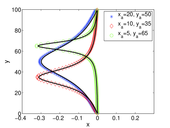
Figure 2: Three examples of deformed grain boundary profiles (symbols) in the case $L=100\gg x_{a}$. The deformation is due to the stress field of an external dislocation positioned at $x=x_{a}$, $y=y_{a}$. The solid lines correspond to the predictions of Eq. (21). 500 pinned extra dislocations (with the same spacing as in the deformable part) have been inserted on both sides of the GB. Notice that there are no fitting parameters.

This result is compared with numerical results from discrete dislocation dynamics simulations of the GB-dislocation system. These are done with a similar setup as e.g. in Ref. [25], with a straight GB as an initial configurations. By letting the GB relax in the stress field of an external dislocation, a good agreement is found (see Fig. 2). Notice that in order for the simulation setup to correspond to Eq. (21) (which was derived by computing the integral from $-\infty$ to $+\infty$), we have considered a system where in addition to the deformable part of the GB of length $L$, there is a large number (here 500) of pinned dislocations on both sides of the deformable part of the GB. The agreement with Eq. (21) is the better the larger the number of these pinned dislocations.

2.3 Correction to the GB field

We are finally able to determine how a dislocation induced deformation affects the stress field generated by the GB. We consider the case in which $L\gg x_{a}$, since it matches are simulation setups. The shear stress at position $(x,y)$ due to the deformed GB is a functional of the displacement field $\eta_{n}$ and can be expressed, by calling $\sigma_{n}$ the shear stress of the $n-$th GB dislocation, as

$$\sigma(x,y)=\sum_{n}\sigma_{n}(x-\eta_{n},y-y_{n}),$$ (22)

where $\eta_{n}$ is given by Equation [21]. Since we are interested in plastic flow activation well inside each grain, we shall assume $\eta_{n}\ll x$, that is we keep far enough from the stress singularities of GB dislocations. This way we can express stress fields through their Taylor expansion around $\eta_{n}\approx 0$ as $\sigma_{n}(x-\eta_{n},y-y_{n})\approx\sigma_{n}(x,y-y_{n})+\sigma_{n}^{\prime}(x,y-y_{n})\eta_{n}+1/2\sigma_{n}^{\prime\prime}(x,y-y_{n})\eta_{n}^{2}+\mathcal{O}(\eta_{n}^{3})$. Equation (22) will be rewritten as

$$\sigma(x,y)=\sigma^{(0)}(x,y)+\sigma^{(1)}(x,y)+\sigma^{(2)}(x,y)+...$$ (23)

where the $i$-th term on the right hand side is obtained summing the $i$-th order as in Equation (22). In passing we note that, given the nature of the derivation operation, in Equation (23) even terms will be odd functions of $x$, while odd terms will be even functions of $x$. Then it is no coincidence that $\sigma^{(0)}(x,y)$ is the well known stress field generated by a straight GB (see References [26, 27]).

As for the first order $\sigma^{(1)}(x,y)$ calculations are not different from the ones carried on in the previous sections. We eventually obtain, in the continuum limit of the sum,

$$\sigma^{(1)}(x,y)=\pi s_{a}x_{a}\frac{\mu b}{1-\nu}\frac{1}{L^{2}}\sum_{l}e^{-\frac{\pi l|x_{a}|}{L}}\sin\frac{\pi ly_{a}}{L}\times$$ (24)

$$\times\,l\left(1-\frac{\pi l|x|}{L}\right)e^{-\frac{\pi l|x|}{L}}\sin\frac{\pi ly}{L}.$$

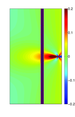
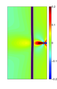
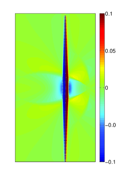
Figure 3: Stress fields of a system consisting of a grain boundary (the dark vertical structure) and an external dislocation positioned to the right side of the grain boundary ($x_{a}=10$, $y_{a}=50$, $L=100$). Left: Stress field in a situation where the grain boundary is not allowed to deform. Middle: Stress field with a deformable grain boundary. Right: The difference of the absolute values of the two stress fields, $|\sigma^{deformed}|-|\sigma^{undeformed}|$. Negative values indicate screening, positive values enhancement of the magnitude of the stress due to grain boundary deformation.

One can observe that this term is, as expected, an even function of $x$. It accounts for corrections observed along the $x$-direction, where the GB deformation produces an even decrease in the absolute value of the shear stress, see Fig. 3 for corresponding results from dislocation dynamics simulations. This is balanced by an increase along the $45$-degree directions along which shear stress is redistributed between adjacent grains. Such corrections are introduced by the $\sigma^{(2)}(x,y)$ term, which can be calculated integrating the second-order term of the expansion of $\sigma_{n}(x-\eta_{n},y-y_{n})$. The procedure does not differ from what we have seen so far, with the exception of some additional complications arising from the fact that this time the sum over $l$ is squared. Skipping the details of the calculation, we obtain

$$\sigma^{(2)}(x,y)=2s\pi^{2}x_{a}^{2}\frac{\mu b}{1-\nu}\frac{D}{L^{4}}\sum_{l}\sum_{\lambda}e^{-\frac{\pi(l+\lambda)|x_{a}|}{L}}\sin\frac{\pi ly_{a}}{L}\sin\frac{\pi\lambda y_{a}}{L}\times$$ (25)

$$\times\,\mbox{sign}(x)\left[(l+\lambda)^{2}e^{-\frac{\pi|l+\lambda||x|}{L}}\left(\frac{\pi}{2}\frac{|l+\lambda|}{L}|x|-1\right)\cos\frac{\pi(l+\lambda)y}{L}-\right.$$

$$\left.-(l-\lambda)^{2}e^{-\frac{\pi|l-\lambda||x|}{L}}\left(\frac{\pi}{2}\frac{|l-\lambda|}{L}|x|-1\right)\cos\frac{\pi(l-\lambda)y}{L}\right],$$

where, as usual, $l,\lambda=1,2,3...N$. Indeed, this term proves to be an odd function of the variable $x$. The same method allows the calculation of further orders of the stress expansion (23) which become relevant as test dislocations are close to the GB, where the anisotropy of stress fields becomes relevant.

We should point out that the terms of the sums over $l$ (and $\lambda$) are exponentially suppressed. As a consequence, sums can be stopped at the first terms. In particular, if the asymmetry or the exact shape of the GB profile are not a concern, the very first terms provide a fair description of the deformed GB. Furthermore, one should notice that the correction itself decays exponentially with the distance of the external dislocation $a$. This suggests the emergence of a screening distance, beyond which the effects of GB deformation do not affect dislocation-GB interaction anymore. This distance is expected to be proportional to $L/(\pi l)$, i.e. higher order corrections in $l$ are weaker at large distance, but may come into play on a shorter range.

3 Discussion

Both analytical calculations and numerical studies of the stress fields of a GB-dislocation system show that the GB deformation tends to screen the dominating stress that is causing the deformation. At the same time, due to the fact that a stress field of an edge dislocation has both positive and negative regions, some parts of such a stress field are also enhanced in the same process. One should note, however, that the strongest effect the GB deformation has is screening close to the deformed part of the GB. This happens on both sides of the GB (see Fig. 3).

The implications for collective dynamics in polycrystals with flexible grain boundaries would then be the following: Low angle GB’s tend to accommodate the excess stresses within a grain by deforming in such a way that such excess stresses are partly screened. This screening effect is exponentially suppressed beyond a length that is of the order of the typical grain size $\sim L$, and has a magnitude scaling as $\sim 1/L$. Consequently, in addition to acting as boundaries to the dislocations themselves, deformable GB’s tend to hinder also stresses from being transferred from one grain to another. This effect gets stronger with decreasing grain size. One should note, however, that also various dislocation arrangements present within grains tend to screen the long range stress fields typical to these systems.

The behavior of this simple model system is hence controlled mainly by a single parameter, namely the typical grain size $\sim L$. In fact, our results suggest that deformable low angle GB’s tend to confine avalanches of plastic activity to some extent within single grains. This could be anticipated to be the case also for general (high angle) grain boundaries: even if they cannot be thought as deformable arrays of mobile dislocations, the large difference in the respective orientations of neighboring grains means that only a fraction of the stress is effectively transferred over such a GB.

Recent experiments on polycrystalline ice reveal an intriguing crossover in the AE amplitude distributions: Small and large avalanches appear to be characterized by different power law exponents [9]. The observation that small avalanches are described by the same exponent as avalanches in single crystal samples leads to the natural conclusion that such small avalanches do not feel the presence of the GB’s. On the other hand, larger avalanches will necessarily interact with the GB’s. In the experiment presented in Ref. [9], the exponent describing such large avalanches was found to be smaller as compared to the one describing the statistics of smaller avalanches.

Thus, the presence of GB’s will change the statistics of avalanches in some way. One possibility, along similar ideas as presented in Ref. [9], is to consider the spreading process on a coarse-grained scale of grains. An initial avalanche within a grain, if reaching the region close enough to a grain boundary, may spread to neighboring grains thus triggering avalanches there. Triggering is governed by an effective spreading probability $p$ that depends (among other things) on the details of the dislocation-grain boundary interaction discussed above. Hence the ensuing spreading process is characterized by an average $p$ and geometrical factors (correlations in GB orientations, grain sizes and their correlations etc.). This leads to a number $N$ of grains that participate in the “total” avalanche. The statistics of $N$ will follow at the simplest a mean-field branching process for which one in general has three possible scenarios: i) a sub-critical process with $\langle N\rangle=\mathrm{const}$, ii) an exactly critical process with $P(N)\sim N^{-3/2}$, iii) a supercritical process which never stops. Clearly, the last case can be excluded by common sense. As for the the first two options, it appears much more likely that the grain-to-grain spreading is actually sub-critical. This would be in agreement with the observation that in experiments of Ref. [9] a grain-size dependent cut-off for the acoustic emission amplitudes was observed. On the other hand, this would indicate that the observed avalanche distributions would not change from what one sees on a single grain level.

In conclusion, we have considered the GB mediated dislocation interactions for a “toy” system in two dimensions. This has allowed us to make analytical progress, to compare with numerics, and to understand the nature of screening. Regardless of the obvious limitations of the simple model studied here, working out these problems leads to an increased understanding of the physics of avalanches in the plasticity of polycrystalline materials. Clearly, there is much room for short-term investigations in three separate directions at least. One is the accumulation of further experimental data on these phenomena. The second is the influence of the geometry (dimension, GB angle, grain size, correlations) on these processes, which can be studied partly experimentally and partly by numerical, atomistic, simulations. Finally, there seems to be room for the development of coarse-grained models which would match their predictions with experimental data.

Acknowledgements - The authors would like to acknowledge the support of the Center of Excellence -program of the Academy of Finland, and the financial support of the European Commissions NEST Pathfinder programme TRIGS under contract NEST-2005-PATH-COM-043386. MJA and LL would like to thank the ISI institute (Turin, Italy) for hospitality. PM is grateful to the Laboratory of Physics, Helsinki University of Technology (Finland) for kind hospitality and acknowledges financial support from the Ministerio de Educación y Ciencia (Spain), under grant FIS2007-66485-C02-02.

Appendix

In several cases in the derivations, sums have been replaced by integrals to infinity. While the validity of the infinity assumption is quite intuitive if $L$ is taken significantly larger than $x_{a}$, the transition to continuum requires a few words of discussion. Provided that the sum is extended to infinity, we calculate it using the Poisson integral relation (see [27])

$$\sum_{n=-\infty}^{\infty}f(n)=\sum_{k=-\infty}^{\infty}\int_{-\infty}^{\infty}\!dn\,f(n)e^{2i\pi kn}.$$ (26)

Calculating the integral first, we always obtain an exponential $\approx e^{i\pi kx/D}$ term, which rapidly goes to zero if $k$ is increased, as we always assumed $x\gg D$. As a result, the $k=0$ term of the sum over $k$ alone provides a good estimate of the initial sum. But this is equivalent, as it can be easily noticed, to replacing the sum with an integral in the first place.

Figure 1: A schematic diagram of the grain boundary dislocation system. The GB is modelled as a discrete linear assembly of $N+1$ edge dislocations distributed along the $y$ direction, with Burgers vectors $\vec{b}$ parallel to the $x$ axis. Dislocation spacing is $D$. The endpoint dislocations of the GB, positioned at $y=0$ and $y=L$, are fixed to $x=0$. The rest of the GB dislocations are allowed to move in the $x$ direction as a response to the stress field of the external dislocation positioned at $x=x_{a}$, $y=y_{a}$. The ensuing GB displacement in the $x$ direction is represented by the vector $\vec{\eta}$, with components $\eta_{n}$ corresponding to the displacement of the $n$th dislocation.

References

- [1] J. Weiss, and J. R. Grasso, J. Phys. Chem. 101, 6113 (1997).
- [2] M.-C. Miguel et al., Nature 410, 667 (2001).
- [3] M. D. Uchic et al., Science 305, 986 (2004).
- [4] D. M. Dimiduk et al., Science 312, 1188 (2006).
- [5] R. F. Tinder, and J. P. Trzil, Acta Metall. 21, 975 (1973).
- [6] H. H. Potthoff, Phys. Stat. Sol. (a) 77, 215 (1983).
- [7] J. Weiss, and D. Marsan, Science 299, 89 (2003).
- [8] M. Zaiser et al., Phys. Rev. Lett 93, 195507 (2004).
- [9] T. Richeton et al., Nature Mater. 4, 465 (2005).
- [10] F. F. Csikor et al., Science 318, 251 (2007).
- [11] M. Koslowski et al., Phys. Rev. Lett. 93, 125502 (2004).
- [12] M. Zaiser, and P. Moretti, J. Stat. Mech. P08004 (2005).
- [13] E. O. Hall, Proc. Phys. Soc. London Sect. B 64, 747 (1951).
- [14] N. J. Petch, J. Iron Steel Inst., London 173, 25 (1953).
- [15] N. Zhang, Wei Tong, Int. J. Plasticity 20, 523 (2004).
- [16] V. Yamakov et al., Nature Mater. 1 , 1 (2002).
- [17] V. B. Shenoy et al., Phys. Rev. Lett. 80, 742 (1998).
- [18] Z. Shan, et al., Science 305, 654 (2004).
- [19] F. Leoni and S. Zapperi, J. Stat. Mech. P12004 (2007).
- [20] F. Louchet et al., Phys. Rev. Lett. 97, 075504 (2006).
- [21] P. Lipowsky et al., Nature Mater. 4, 407 - 411 (2005).
- [22] P. Moretti et al., Phys. Rev. B 72, 014505 (2005).
- [23] R. Bruinsma, B. I. Halperin, and A. Zippelius, Phys. Rev. B 25, 579 (1982)
- [24] A. L. Fetter, and J. D. Walecka, Theoretical Mechanics for Particles and Continua; McGraw-Hill Companies (February 1, 1980)
- [25] M.-C. Miguel, et al., Phys. Rev. Lett. 89, 165501 (2002).
- [26] J. P. Hirth, and J. Lothe, Theory of Dislocations, Krieger Publishing Company; (May 1992)
- [27] L. D. Landau, E. M. Lifshitz, Theory of Elasticity, Butterworth-Heinemann; (January 1, 1986)