An Improved Scheme for Initial Ranging in OFDMA-based Networks

Abstract

An efficient scheme for initial ranging has recently been proposed by X. Fu et al. in the context of orthogonal frequency-division multiple-access (OFDMA) networks based on the IEEE 802.16e-2005 standard. The proposed solution aims at estimating the power levels and timing offsets of the ranging subscriber stations (RSSs) without taking into account the effect of possible carrier frequency offsets (CFOs) between the received signals and the base station local reference. Motivated by the above problem, in the present work we design a novel ranging scheme for OFDMA in which the ranging signals are assumed to be misaligned both in time and frequency. Our goal is to estimate the timing errors and CFOs of each active RSS. Specifically, CFO estimation is accomplished by resorting to subspace-based methods while a least-squares approach is employed for timing recovery. Computer simulations are used to assess the effectiveness of the proposed solution and to make comparisons with existing alternatives.

I Introduction

The main impairment of an orthogonal frequency-division multiple-access (OFDMA) network is represented by its remarkable sensitivity to timing errors and carrier frequency offsets (CFOs) between the uplink signals and the base station (BS) local references. For this reason, the IEEE 802.16e-2005 standard for OFDMA-based wireless metropolitan area networks (WMANs) specifies a synchronization procedure called Initial Ranging (IR) where subscriber stations that intend to establish a link with the BS can use some dedicated subcarriers to transmit their specific ranging codes [1]. Once the BS has revealed the presence of ranging subscriber stations  (RSSs), it has to estimate some fundamental parameters including timing errors, CFOs and power levels.

Two prominent schemes for initial synchronization and power control in OFDMA were proposed in [2] and [3]. In these works, a long pseudo-noise sequence is transmitted by each RSS over the available ranging subcarriers. Timing recovery is then accomplished on the basis of suitable correlations computed in the frequency- and time-domain, respectively. The main drawback of these methods is their sensitivity to multipath distortion, which destroys orthogonality among the employed codes and gives rise to multiple access interference (MAI). Better results are obtained in [4] by using a set of generalized chirp-like (GCL) sequences, which echibits increased robustness against the channel selectivity. A different approach to managing the IR process has recently been proposed in [5]. Here, the pilot streams transmitted by RSSs are spread in the time-domain over adjacent OFDM blocks using orthogonal codes. In this way, signals of different RSSs can be easily separated at the BS as they remain orthogonal after propagating through the channel. Timing information is eventually acquired in an iterative fashion by exploiting the autocorrelation properties of the received samples induced by the use of the cyclic prefix (CP). Unfortunately, this scheme is derived under the assumption of perfect frequency alignment between the received signals and the BS local reference. Actually, the occurrence of residual CFOs results into a loss of orthogonality among ranging codes and may lead to severe degradations of the system performance in terms of mis-detection probability and estimation accuracy.

In the present work we propose a novel ranging scheme for OFDMA systems that is robust to time and frequency misalignments. The goal is to estimate timing errors and CFOs of all active RSSs. The number of active codes is found by resorting to the minimum description length (MDL) principle [6] while the multiple signal classification (MUSIC) algorithm [7] is employed to detect which codes are actually active and to determine their corresponding CFOs. Timing estimation is eventually achieved through least-squares (LS) methods. Although the proposed solution allows one to estimate the timing errors of each RSS in a decoupled fashion, it may involve huge computational burden in applications characterized by large propagation delays. For this reason, we also present an alternative scheme derived from ad hoc-reasoning which results into substantial computational saving. It is worth noting that timing synchronization in OFDMA uplink transmissions has received little attention so far. A well-established way to handle timing errors is to design the CP length large enough to include both the channel delay spread and the two-way propagation delay between the BS and the user station [8]. This leads to a quasi-synchronous system in which timing errors can be viewed as part of the channel impulse response (CIR) and are compensated for by the channel equalizer. Unfortunately, this approach poses an upper limit to the maximum tolerable propagation delay or, equivalently, to the maximum distance between the BS and the subscriber stations [9]. For this reason, its application to a scenario with large cells (as envisioned in next broadband wireless networks) is hardly viable. In the latter case, accurate knowledge of the timing errors is required in order to align the uplink signals to the BS time scale.

II System description and signal model

II-A System description

The investigated OFDMA network employs $N$ subcarriers with frequency spacing $\Delta f$ and indices in the set $\mathcal{J}=\{0,1,\ldots,N-1\}$. Following [5], we denote $R$ the number of subchannels reserved for the IR process. Each subchannel is divided into $Q$ subbands uniformly spaced over the signal bandwidth at a distance $(N/Q)\Delta f$ from each other. A given subband is composed of a set of $V$ adjacent subcarriers. The subcarrier indices within the $q$th subband $(q=0,1,\ldots,Q-1)$ of the $r$th ranging subchannel $(r=0,1,\ldots,R-1)$ are collected into a set $\mathcal{J}_{q}^{(r)}=\{i_{q,\nu}^{(r)}~{};\nu=0,1,\ldots,V-1\}$ with entries

$$i_{q,\nu}^{(r)}=\frac{qN}{Q}+\frac{rN}{QR}+\nu.$$ (1)

The $r$th subchannel is thus composed of subcarriers with indices taken from $\mathcal{J}^{(r)}={\cup_{q=0}^{Q-1}\mathcal{J}_{q}^{(r)}}$. Hence, a total of $N_{R}=QVR$ ranging subcarriers are available in the system with indices in the set $\mathcal{J}_{R}={\cup_{r=0}^{R-1}\mathcal{J}^{(r)}}$. The remaining $N-N_{R}$ subcarriers are used for data transmission and are assigned to data subscriber stations (DSSs) which have already completed their IR process and are assumed to be perfectly synchronized to the BS time and frequency scales [5].

We denote by $M$ the number of consecutive OFDM blocks reserved for IR and assume that each ranging subchannel can be accessed at most by $M-1$ RSSs. The latter are separated by means of specific ranging codes selected in a pseudo-random fashion from a predefined set $\{\mathbf{c}_{1},\mathbf{c}_{2},\ldots,\mathbf{c}_{M-1}\}$, with $\mathbf{c}_{k}=[c_{k}(1),\,c_{k}(2),\ldots,c_{k}(M)]^{T}$ (the superscript ^T denotes the transpose operation). As in [5], we assume that different RSSs employ different codes. Without loss of generality, in what follows we concentrate on the $r$th ranging subchannel and denote by $K^{(r)}\leq M-1$ the number of simultaneously active RSSs. Also, to simplify the notation, the subchannel index ^(r) is dropped in all subsequent derivations.

The waveform transmitted by the $k$th RSS ($1\leq k\leq K$) propagates through a multipath channel characterized by an impulse response $\mathbf{h}_{k}=[h_{k}(0),h_{k}(1),\ldots,h_{k}(L-1)]^{T}$ of length $L$ (in sampling periods). At the BS, the received samples are not synchronized with the local references. We denote by $\theta_{k}$ the timing error expressed in sampling periods while $\varepsilon_{k}$ is the frequency offset normalized to the subcarrier spacing. As discussed in [8], subscriber stations that intend to start the ranging process compute initial frequency and timing estimates on the basis of a downlink control signal broadcast by the BS. The estimated parameters are then employed by each RSS as synchronization references for the uplink ranging transmission. This means that during IR the CFOs are only due to Doppler shifts and/or estimation errors and, in consequence, they are assumed to lie within a small fraction of the subcarrier spacing. Furthermore, in order to eliminate interblock interference (IBI), we assume that during the ranging process the CP length comprises $N_{G}\geq\theta_{\max}+L$ sampling periods, where $\theta_{\max}$ is the maximum expected timing error [9]. This assumption is not restrictive, since in many standardized OFDM systems the initialization blocks are usually preceded by long CPs.

II-B Signal model

We denote by $\mathbf{Y}_{m}$ the $QV$-dimensional vector that collects the DFT outputs corresponding to the considered subchannel during the $m$th OFDM block. Since the DSSs are assumed to be perfectly synchronized to the BS references, their signals will not contribute to $\mathbf{Y}_{m}$. In contrast, the presence of uncompensated CFOs destroys orthogonality among ranging signals, thereby leading to some interchannel interference (ICI). However, as the subchannels are well separated in the frequency domain, we can reasonably neglect interference on $\mathbf{Y}_{m}$ arising from ranging signals of subchannels other than the considered one. Under this assumption, we may write

$$\mathbf{Y}_{m}=\sum\limits_{k=1}^{K}{c_{k}(m)e^{j{m\omega_{k}N_{T}}}\mathbf{A}(\omega_{k})\mathbf{S}_{k}}(\theta_{k})+\mathbf{n}_{m}$$ (2)

where $\omega_{k}=2\pi\varepsilon_{k}/N$, $N_{T}=N+N_{G}$ is the duration of the cyclically extended block and $\mathbf{n}_{m}$ is a Gaussian vector with zero mean and covariance matrix $\sigma^{2}\mathbf{I}_{QV}$ (we denote by $\mathbf{I}_{N}$ the identity matrix of order $N$). Also, we have defined

$$\mathbf{A}(\omega_{k})=\mathbf{F}\mathbf{V}(\omega_{k})\mathbf{F}^{H}$$ (3)

where $\mathbf{V}(\omega_{k})$ accounts for the CFOs and is given by

$$\mathbf{V}(\omega_{k})=\mathrm{diag}\left\{{e^{j{n}\omega_{k}};n=0,1,\ldots,N-1}\right\}$$ (4)

while $\mathbf{F}=\left[{\mathbf{F}_{0}^{H},\mathbf{F}_{1}^{H},\ldots,\mathbf{F}_{Q-1}^{H}}\right]^{H}$ (the superscript ^H denotes the Hermitian transposition) with $\mathbf{F}_{q}$ ($q=0,1,\ldots,Q-1)$ denoting a $V\times N$ matrix with entries

$$\left[{\mathbf{F}}_{q}\right]_{\nu,n}=\frac{1}{\sqrt{N}}e^{-j{2\pi n}i_{q,\nu}/N}\quad 0\leq\nu\leq V-1,0\leq n\leq N-1.$$ (5)

Vector $\mathbf{S}_{k}(\theta_{k})$ in (2) can be partitioned as $\mathbf{S}_{k}(\theta_{k})=\left[\mathbf{S}_{k}^{T}(\theta_{k},i_{1}),\mathbf{S}_{k}^{T}(\theta_{k},i_{2}),\ldots,\mathbf{S}_{k}^{T}(\theta_{k},i_{Q-1})\right]^{T}$, where $\mathbf{S}_{k}(\theta_{k},i_{q})$ is a $V$-dimensional vector with elements

$$S_{k}(\theta_{k},i_{q,\nu})=e^{-j{2\pi\theta_{k}}i_{q,\nu}/N}H_{k}(i_{q,\nu}),\quad 0\leq\nu\leq V-1$$ (6)

while $H_{k}(i_{q,\nu})$ denotes the channel frequency response over the $i_{q,\nu}$th subcarrier and is given by

$$H_{k}(i_{q,\nu})=\sum_{\ell=0}^{L-1}h_{k}(\ell)e^{-j{2\pi\ell}i_{q,\nu}/N}.$$ (7)

From (6) we see that $\theta_{k}$ simply appears as a phase shift across the DFT outputs. The reason is that the CP length is larger than the maximal expected propagation delay, thereby making the ranging signals quasi-synchronous.

In the following sections we show how vectors $\{\mathbf{Y}_{m}\}_{m=0}^{M-1}$ can be exploited to compute frequency and timing estimates for all active ranging codes.

III Estimation of the CFOs

To simplify the derivation, we assume that the CFOs are adequately smaller than the subcarrier spacing, i.e., $\left|{\omega_{k}}\right|\ll 1$. In such a case, matrices $\mathbf{A}(\omega_{k})$ in (3) can reasonably be replaced by $\mathbf{I}_{N}$ to obtain [8]

$$\mathbf{Y}_{m}\approx\sum\limits_{k=1}^{K}{c_{k}(m)e^{j{m\omega_{k}N_{T}}}\mathbf{S}_{k}}(\theta_{k})+\mathbf{n}_{m}.$$ (8)

This equation indicates that each CFO results only in a phase shift between contiguous OFDM blocks. Collecting the $i_{q,\nu}$th DFT output of all $M$ ranging blocks into a vector $\mathbf{Y}(i_{q,\nu})=[Y_{0}(i_{q,\nu}),Y_{1}(i_{q,\nu}),\ldots,Y_{M-1}(i_{q,\nu})]^{T}$, we may write

$$\mathbf{Y}(i_{q,\nu})=\sum_{k=1}^{K}S_{k}(\theta_{k},i_{q,\nu})\mathbf{\Gamma}(\omega_{k})\mathbf{c}_{k}+\mathbf{n}(i_{q,\nu})$$ (9)

where $\mathbf{n}(i_{q,\nu})$ is Gaussian distributed with zero-mean and covariance matrix $\sigma^{2}\mathbf{I}_{M}$, while $\mathbf{\Gamma}(\omega_{k})=\text{diag}\{e^{j{m\omega_{k}N_{T}}}~{};m=0,1,\ldots,M-1\}$ is a diagonal matrix that accounts for the phase shifts induced by $\omega_{k}$.

Inspection of (9) reveals that, apart from thermal noise, vector $\mathbf{Y}(i_{q,\nu})$ is a linear combination of the frequency-rotated codes $\{\mathbf{\Gamma}(\omega_{k})\mathbf{c}_{k}\}$. This means that the signal space is spanned by the $K$ vectors $\{\mathbf{\Gamma}(\omega_{k})\mathbf{c}_{k}\}$ that correspond to the active RSSs [10]. Then, if we temporarily assume that the number $K$ of active codes is known at the receiver, an estimate of $\omega_{k}$ ($k=1,2,\ldots,K$) can be obtained by resorting to the MUSIC algorithm [7]. To see how this comes about, we use the observations $\{\mathbf{Y}(i_{q,\nu})\}$ to obtain the following sample correlation matrix

$$\hat{\mathbf{R}}_{Y}=\frac{1}{QV}\sum_{v=0}^{V-1}\sum_{q=0}^{Q-1}\mathbf{Y}(i_{q,\nu})\mathbf{Y}^{H}(i_{q,\nu}).$$ (10)

Next, based on the forward-backward (FB) approach [10], we compute

$$\widetilde{\mathbf{R}}_{Y}=\frac{1}{2}(\hat{\mathbf{R}}_{Y}+\mathbf{J}\hat{\mathbf{R}}_{Y}^{T}\mathbf{J})$$ (11)

where $\mathbf{J}$ is the exchange matrix with 1’s on the anti-diagonal and 0’s elsewhere. We denote by $\lambda_{1}\geq\lambda_{2}\geq\cdots\geq\lambda_{M}$ the eigenvalues of $\widetilde{\mathbf{R}}_{Y}$ arranged in non-increasing order, and by $\{\mathbf{s}_{1},\mathbf{s}_{2},\ldots,\mathbf{s}_{M}\}$ the corresponding eigenvectors. The MUSIC algorithm relies on the fact that the eigenvectors associated with the $M-K$ smallest eigenvalues are an estimated basis of the noise subspace and, accordingly, they are approximately orthogonal to all vectors in the signal space [7]. Hence, an estimate of $\omega_{k}$ is obtained by minimizing the projection of $\mathbf{\Gamma}(\widetilde{\omega})\mathbf{c}_{k}$ onto the noise subspace, i.e.,

$$\hat{\omega}_{k}=\arg\underset{\widetilde{\omega}}{\max}\left\{\Psi_{k}(\widetilde{\omega})\right\},$$ (12)

with

$$\Psi_{k}(\widetilde{\omega})=\frac{1}{\sum_{m=K+1}^{M}\left|\mathbf{c}_{k}^{H}\mathbf{\Gamma}^{H}(\widetilde{\omega})\mathbf{s}_{m}\right|^{2}}.$$ (13)

It is worth observing that CFO recovery must be accomplished for any active RSS. However, since the BS has no prior knowledge as to which codes have been transmitted in the considered subchannel, it must evaluate the quantities $\{\hat{\omega}_{{1}},\hat{\omega}_{{2}},\ldots,\hat{\omega}_{{M-1}}\}$ for the complete set $\{\mathbf{c}_{1},\mathbf{c}_{2},\ldots,\mathbf{c}_{M-1}\}$. At this stage the problem arises of identifying which codes are actually active. The identification algorithm looks for the $K$ largest values in the set $\{\Psi_{k}(\hat{\omega}_{k})\}_{k=1}^{M-1}$, say $\{\Psi_{u_{k}}(\hat{\omega}_{u_{k}})\}_{k=1}^{K}$, and declare as active the corresponding codes $\{\mathbf{c}_{u_{k}}\}_{k=1}^{K}$. The CFO estimates are eventually found as $\hat{\boldsymbol{\omega}}_{u}=\mathbf{[}\hat{\omega}_{u_{1}},\hat{\omega}_{u_{2}},\ldots,\hat{\omega}_{u_{K}}\mathbf{]}^{T}$.

At this stage we are left with the problem of estimating the parameter $K$ to be used in (13). For this purpose, we adopt the MDL approach and obtain [6]

$$\hat{K}=\arg\underset{\tilde{K}}{\min}\left\{\mathcal{F(}\tilde{K})\right\}$$ (14)

where $\mathcal{F(}\tilde{K})$ is the following metric

$$\mathcal{F(}\tilde{K})=\frac{1}{2}\tilde{K}(2M-\tilde{K})\ln(QV)-QV(M-\tilde{K})\ln\rho(\tilde{K})$$ (15)

with $\rho(\tilde{K})$ denoting the ratio between the geometric and arithmetic mean of $\{\lambda_{\tilde{K}+1},\lambda_{\tilde{K}+2},\ldots,\lambda_{M}\}$. Finally, replacing $K$ by $\hat{K}$ in (13) leads to the proposed MUSIC-based frequency estimator (MFE) while the described identification algorithm is called the MUSIC-based code detector (MCD)

IV Estimation of the timing delays

After code detection and CFO recovery, the BS must acquire information about the timing delays of all ranging signals. This problem is now addressed by resorting to LS methods. In doing so we still assume that the number of active codes has been correctly estimated so that $\hat{K}=K$. Also, to simplify the notation, the indices $\{u_{k}\}_{k=1}^{K}$ of the detected codes are relabeled following the map $u_{k}\longrightarrow k$ for $k=1,2,\ldots,K$.

We begin by reformulating (9) in a more compact form. For this purpose, we collect the CFOs and timing errors in two $K$-dimensional vectors ${\boldsymbol{\omega}=[}\omega_{1},\omega_{2},\ldots,\omega_{K}\mathbf{]}^{T}$ and $\boldsymbol{\theta}=[\theta_{1},\theta_{2},\ldots,\theta_{K}]^{T}$. Then, after defining the matrix $\mathbf{C}({\boldsymbol{\omega}})=\left[\mathbf{\Gamma}(\omega_{{1}})\mathbf{c}_{{1}}~{}~{}\mathbf{\Gamma}(\omega_{{2}})\mathbf{c}_{{2}}~{}\cdots~{}\mathbf{\Gamma}(\omega_{{K}})\mathbf{c}_{{K}}\right]$ and the vector $\mathbf{S}(\boldsymbol{\theta},i_{q,\nu})=[S_{{1}}(\theta_{1},i_{q,\nu}),S_{{2}}(\theta_{2},i_{q,\nu}),\ldots,S_{{K}}(\theta_{K},i_{q,\nu})]^{T}$, we may rewrite (9) in the equivalent form

$$\mathbf{Y}(i_{q,\nu})=\mathbf{C}(\boldsymbol{\omega})\mathbf{S}(\boldsymbol{\theta},i_{q,\nu})+\mathbf{n}(i_{q,\nu}).$$ (16)

Omitting for simplicity the functional dependence of $\mathbf{S}(\boldsymbol{\theta},i_{q,\nu})$ on $\boldsymbol{\theta}$ and assuming $\hat{\boldsymbol{\omega}}\approx\boldsymbol{\omega}$, from (16) the maximum likelihood estimate of $\mathbf{S}(i_{q,\nu})$ is found to be

$$\hat{\mathbf{S}}(i_{q,\nu})=[\mathbf{C}^{H}(\hat{\boldsymbol{\omega}})\mathbf{C}(\hat{\boldsymbol{\omega}})]^{-1}\mathbf{C}^{H}(\hat{\boldsymbol{\omega}})\mathbf{Y}(i_{q,\nu}).$$ (17)

Substituting (16) into (17) yields

$$\hat{\mathbf{S}}(i_{q,\nu})=\mathbf{S}(i_{q,\nu})+\boldsymbol{\xi}(i_{q,\nu})$$ (18)

where $\boldsymbol{\xi}(i_{q,\nu})$ is a zero-mean disturbance term. From (6) and (7) it follows that

$$\hat{S}_{{k}}(i_{q,\nu})=e^{-j\frac{{2\pi\theta_{k}}}{N}i_{q,\nu}}\sum_{\ell=0}^{L-1}h_{k}(\ell)e^{-j\frac{{2\pi n}}{N}i_{q,\nu}}+\xi_{{k}}(i_{q,\nu}).$$ (19)

On denoting $\hat{\mathbf{S}}_{{k}}(\nu)=\left[\hat{S}_{{k}}(i_{0,\nu}),\hat{S}_{{k}}(i_{1,\nu}),\ldots,\hat{S}_{{k}}(i_{Q-1,\nu})\right]^{T},$ and $\boldsymbol{\Phi}(\theta_{{k}},\nu)=\mathrm{diag}\{e^{-j\frac{{2\pi\theta_{{k}}}}{N}i_{q,\nu}}~{};~{}q=0,1,\ldots,Q-1\}$, we may rewrite (19) as follows

$$\hat{\mathbf{S}}_{{k}}(\nu)=\boldsymbol{\Phi}(\theta_{{k}},\nu)\mathbf{F}(\nu)\mathbf{h}_{{k}}+\boldsymbol{\xi}_{{k}}(\nu)$$ (20)

where $\boldsymbol{\xi}_{{k}}(\nu)=[\xi_{{k}}(i_{0,\nu}),\xi_{{k}}(i_{1,\nu}),\ldots,\xi_{{k}}(i_{Q-1,\nu})]^{T}$ while $\mathbf{F}(\nu)$ is a matrix of dimension $Q\times L$ with entries $[\mathbf{F}(\nu)]_{q,\ell}=e^{-j\frac{{2\pi\ell}}{N}i_{q,\nu}}$ for $0\leq q\leq Q-1$ and $0\leq\ell\leq L-1$

Equation (20) indicates that, apart from the disturbance term $\boldsymbol{\xi}_{{k}}(\nu)$, $\hat{\mathbf{S}}_{{k}}(\nu)$ is only contributed by the ${k}$th RSS, meaning that ranging signals have been successfully decoupled at the BS. We may thus exploit vectors $\{\hat{\mathbf{S}}_{{k}}(\nu)~{};~{}\nu=0,1,\ldots,V-1\}$ to get LS estimates of $(\theta_{{k}},\mathbf{h}_{{k}})$ separately for each RSS. This amounts to minimizing the following objective function with respect to $(\tilde{\theta}_{{k}},\tilde{\mathbf{h}}_{{k}})$

$$\Lambda_{{k}}(\tilde{\theta}_{{k}},\tilde{\mathbf{h}}_{{k}})=\sum_{\nu=0}^{V-1}\left\|\hat{\mathbf{S}}_{{k}}(\nu)-\boldsymbol{\Phi}(\tilde{\theta}_{{k}},\nu)\mathbf{F}(\nu)\tilde{\mathbf{h}}_{{k}}\right\|^{2}.$$ (21)

For a fixed $\tilde{\theta}_{{k}}$, the minimum of $\Lambda_{{k}}(\tilde{\theta}_{{k}},\tilde{\mathbf{h}}_{{k}})$ is achieved at

$$\hat{\mathbf{h}}_{{k}}=\frac{1}{QV}\sum_{\nu=0}^{V-1}\mathbf{F}^{H}(\nu)\boldsymbol{\Phi}^{H}(\tilde{\theta}_{{k}},\nu)\hat{\mathbf{S}}_{{k}}(\nu)$$ (22)

where we have used the identity $\mathbf{F}^{H}(\nu)\mathbf{F}(\nu)=Q\cdot\mathbf{I}_{L}$. Then, substituting (22) into (21) and minimizing with respect to $\tilde{\theta}_{k}$ yields the timing estimate in the form

$$\hat{\theta}_{k}=\arg\underset{0\leq\tilde{\theta}_{k}\leq\theta_{\max}}{\max}\left\{\Upsilon(\tilde{\theta}_{k})\right\}$$ (23)

where $\Upsilon(\tilde{\theta}_{k})$ is given by

$$\Upsilon(\tilde{\theta}_{k})=\sum_{\ell=\tilde{\theta}_{k}}^{\tilde{\theta}_{k}+L-1}\left|\sum_{\nu=0}^{V-1}\hat{s}_{k}(\nu,\ell)e^{j2\pi\ell\nu/N}\right|^{2}$$ (24)

and we have denoted by $\hat{s}_{k}(\nu,\ell)$ the $Q$-point IDFT of the sequence $\{\hat{S}_{k}(i_{q,\nu});0\leq q\leq Q-1\}$. In the sequel $\hat{\theta}_{k}$ is termed the LS-based timing estimator (LS-TE).

Once $\hat{\theta}_{k}$ has been computed from (23), it is used in (22) to estimate the CIR of the $k$th RSS as

$$\hat{\mathbf{h}}_{k}=\frac{1}{QV}\sum_{\nu=0}^{V-1}\mathbf{F}^{H}(\nu)\boldsymbol{\Phi}^{H}(\hat{\theta}_{k},\nu)\hat{\mathbf{S}}_{k}(\nu).$$ (25)

It is worth noting that for $V=1$ the timing metric (24) reduces to

$$\left.\Upsilon(\tilde{\theta}_{k})\right|_{V=1}=\sum_{\ell=\tilde{\theta}_{k}}^{\tilde{\theta}_{k}+L-1}\left|\hat{s}_{k}(0,\ell)\right|^{2}$$ (26)

and becomes periodic in $\tilde{\theta}_{k}$ with period $Q$. In such a case, the estimate $\hat{\theta}_{k}$ is affected by an ambiguity of multiples of $Q$. This ambiguity does not represent a serious problem as long as $Q$ can be chosen to be greater than $\theta_{\max}$. Unfortunately, in some applications this may not be the case. For example, in [5] we have $Q=8$ while $\theta_{\max}=102$.

IV-A Reduced-complexity timing estimation

Although separating the RSS signals at the BS considerably reduces the system complexity, evaluating $\Upsilon(\tilde{\theta}_{k})$ for $\tilde{\theta}_{k}=0,1,\ldots,\theta_{\max}$ may still be computationally demanding, especially in applications where $\theta_{\max}$ is large. For this reason, we now develop an ad-hoc reduced complexity timing estimator (RC-TE).

We begin by decomposing the timing error $\theta_{k}$ into a fractional part $\beta_{k}$, less than $Q$, plus an integer part which is multiple of $Q$, i.e.,

$$\theta_{k}=\beta_{k}+p_{k}Q$$ (27)

where $\beta_{k}\in\{0,1,\ldots,Q-1\}$ while $p_{k}$ is an integer parameter taken from $\{0,1,\ldots,P-1\}$ with $P=\left\lfloor\theta_{\max}/Q\right\rfloor$. Omitting the details, it is possible to rewrite $\Upsilon(\tilde{\theta}_{k})$ as

$$\Upsilon(\tilde{\theta}_{k})=\Upsilon_{1}(\tilde{\beta}_{k})+\Upsilon_{2}(\tilde{\beta}_{k},\tilde{p}_{k})$$ (28)

where

$$\Upsilon_{1}(\tilde{\beta}_{k})=\sum_{\ell=\tilde{\beta}_{k}}^{\tilde{\beta}_{k}+L-1}\sum_{\nu=0}^{V-1}\left|\hat{s}_{k}(\nu,\ell)\right|^{2}$$ (29)

while $\Upsilon_{2}(\tilde{\beta}_{k},\tilde{p}_{k})$ is shown in (30) at the top of the next page.

$$\Upsilon_{2}(\tilde{\beta}_{k},\tilde{p}_{k})=2\Re e\left\{\sum_{\ell=\tilde{\beta}_{k}}^{\tilde{\beta}_{k}+L-1}\sum_{\nu=0}^{V-2}\sum_{n=1}^{V-\nu-1}\hat{s}_{k}(\nu,\ell)\hat{s}_{k}^{\ast}(\nu+n,\ell)e^{-j2\pi n(\ell+\tilde{p}_{k}Q)/N}\right\}$$ (30)

The RC-TE is a suboptimal scheme which, starting from (28), estimates $\beta_{k}$ and $p_{k}$ in a decoupled fashion. More precisely, an estimate of $\beta_{k}$ is first obtained looking for the maximum of $\Upsilon_{1}(\tilde{\beta}_{k})$, i.e.,

$$\hat{\beta}_{k}=\arg\underset{0\leq\tilde{\beta}_{k}\leq Q-1}{\max}\left\{\Upsilon_{1}(\tilde{\beta}_{k})\right\}.$$ (31)

Next, replacing $\beta_{k}$ with $\hat{\beta}_{k}$ in the right-hand-side of (28) and maximizing with respect to $\tilde{p}_{k}$, provides an estimate of $p_{k}$ in the form

$$\hat{p}_{k}=\arg\underset{0\leq\tilde{p}_{k}\leq P-1}{\max}\left\{\Upsilon_{2}(\hat{\beta}_{k},\tilde{p}_{k})\right\}.$$ (32)

A further reduction of complexity is possible when $V=2$. Actually, in this case it can be shown that maximizing $\Upsilon_{2}(\hat{\beta}_{k},\tilde{p}_{k})$ is equivalent to maximizing $\cos(\varphi_{k}-2\pi\tilde{p}_{k}Q/N)$, where

$$\varphi_{k}=\arg\left\{\sum_{\ell=\hat{\beta}_{k}}^{\hat{\beta}_{k}+L-1}\hat{s}_{k}(0,\ell)\hat{s}_{k}^{\ast}(1,\ell)e^{-j2\pi\ell/N}\right\}.$$ (33)

The estimate of $p_{k}$ is thus obtained in closed-form as

$$\hat{p}_{k}=\frac{N\varphi_{k}}{2\pi Q}.$$ (34)

V Simulation results

V-A System parameters

The simulated system is inspired by [5]. The total number of subcarriers is $N=1024$ while the number of ranging subchannels is $R=8$. Each subchannel is composed by $Q=16$ subbands uniformly spaced at a distance $N/Q=64$. Any subband comprises $V=2$ adjacent subcarriers while the ranging time-slot includes $M=4$ OFDM blocks. The ranging codes are taken from a Fourier set of length $4$ and are randomly selected by the RSSs at each simulation run (expect for the sequence $\left[1,1,1,1\right]^{T}$). The discrete-time CIRs have $L=12$ channel coefficients. The latter are modeled as circularly symmetric and independent Gaussian random variables with zero means (Rayleigh fading) and exponential power delay profiles, i.e., $E\{\left|h_{k}(\ell)\right|^{2}\}=\sigma_{h}^{2}\cdot\exp(-\ell/12)$ with $\ell=0,1,\ldots,11$ and $\sigma_{h}^{2}$ chosen such that $E\{\left\|\mathbf{h}_{k}\right\|^{2}\}=1$. Channels of different users are assumed to be statistically independent. They are generated at each new simulation run and kept fixed over an entire time-slot. The normalized CFOs are uniformly distributed within the interval $[-\Omega,\Omega]$ and vary at each simulation run. We consider a cell radius of 10 km, corresponding to a maximum transmission delay $\theta_{\max}=204$. A CP of length $N_{G}=256$ is chosen to avoid IBI.

Figure 1: $P_{f}$ vs. SNR for $K$ = 2 or 3 when $\Omega$ is 0.05 or 0.075.

V-B Performance evaluation

We begin by investigating the performance of MCD in terms of probability of making an incorrect detection, say $P_{f}$. This parameter is illustrated in Fig. 1 as a function of SNR = $1/\sigma^{2}$ under different operating conditions. The number of active RSSs varies from 2 to 3 while the maximal frequency offset is either $\Omega=0.05$ or $0.075$. Comparisons are made with the ranging scheme discussed by Fu, Li and Minn (FLM) in [5], where the $k$th ranging code is declared active provided that the quantity

$${\mathcal{Z}}_{k}=\frac{1}{M^{2}}\sum\limits_{q=0}^{Q-1}{\sum\limits_{\nu=0}^{V-1}{\left|{\mathbf{c}_{k}^{H}\mathbf{Y}(i_{q,\nu})}\right|^{2}}}$$ (35)

exceeds a suitable threshold $\eta$ which is proportional to the estimated noise power $\hat{\sigma}^{2}$. The results of Fig. 1 indicates that the proposed scheme performs remarkably better than FLM because of its intrinsic robustness against CFOs. As expected, the system performance deteriorates for large values of $K$ and $\Omega$. The reason is that increasing $K$ reduces the dimensionality of the noise subspace, which degrades the accuracy of the MUSIC estimator. Furthermore, large CFO values result into significant ICI which is not accounted for in the signal model (8), where $\mathbf{A}(\omega_{k})$ has been replaced by $\mathbf{I}_{N}$.

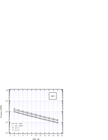
Figure 2: Accuracy of the frequency estimates vs. SNR for $K$ = 2 or 3 when $\Omega$ is 0.05 or 0.075.

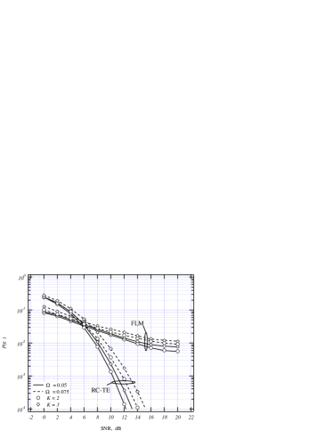
Figure 3: $P(\epsilon)$ vs. SNR for $K$ = 2 or 3 when $\Omega$ is 0.05 or 0.075.

Fig. 2 illustrates the root mean-square-error (RMSE) of the frequency estimates obtained with MFE vs. SNR. Again, we see that the system performance deteriorates when $K$ and $\Omega$ are relatively large. Nevertheless, the accuracy of MFE is satisfactory under all investigated conditions.

The performance of the timing estimators is measured in terms of probability of making a timing error, say $P(\epsilon)$, as defined in [8]. More precisely, an error event is declared to occur whenever the estimate $\hat{\theta}_{k}$ gives rise to IBI during the data section of the frame. In such a case, the quantity $\hat{\theta}_{k}-\theta_{k}+(-N_{G,D}+L)/2$ is larger than zero or smaller than $-N_{G,D}+L-1$, where $N_{G,D}$ is the CP length during the data transmission phase. Fig. 3 illustrates $P(\epsilon)$ vs. SNR as obtained with RC-TE and FLM when $N_{G,D}=64$. The operating conditions are the same of the previous figures. Since the performance of LS-TE is virtually identical to that of RC-TE, it is not reported in order not to overcrowd the figure. We see that for SNR values larger than $6$ dB the proposed scheme provides much better results than FLM.

VI Conclusions

We have derived a novel timing and frequency synchronization scheme for initial ranging in OFDMA-based networks. The proposed solution aims at detecting which codes are actually being employed and provides timing and CFO estimates for all active RSSs. CFO estimation is accomplished by resorting to the MUSIC algorithm while a LS approach is employed for timing recovery. Compared to the timing synchronization algorithm discussed in [5], the proposed scheme is more robust to frequency misalignments and exhibits improved accuracy.

References

- [1] “IEEE standard for local and metropolitan area networks: Air interface for fixed and mobile broadband wireless access systems amendment 2 : Physical and medium access control layers for combined fixed and mobile operation in licensed bands and corrigendum 1,” IEEE Std 802.16e-2005 and IEEE Std. 802.16-2004/Cor 1-2005 Std. 2006, Tech. Rep., 2006.
- [2] J. Krinock, M. Singh, M. Paff, A. Lonkar, L. Fung, and C.-C. Lee, “Comments on OFDMA ranging scheme described in IEEE 802.16ab-01/01r1,” IEEE 802.16 Broadband Wireless Access Working Group, Tech. Rep., July 2001.
- [3] X. Fu and H. Minn, “Initial uplink synchronization and power control (ranging process) for OFDMA systems,” in Proceedings of the IEEE Global Communications Conference (GLOBECOM), Dallas, Texas, USA, Nov. 29 - Dec. 3, 2004, pp. 3999 – 4003.
- [4] D. H. Lee, “OFDMA uplink ranging for IEEE 802.16e using modified generalized chirp-like polyphase sequences,” in Proceedings of the International Conference in Central Asia on Internet (2005), Bishkek, Kyrgyz Republic, Sept. 26 - 29, 2005, pp. 1 – 5.
- [5] X. Fu, Y. Li, and H. Minn, “A new ranging method for OFDMA systems,” IEEE Transactions on Wireless Communications, vol. 6, no. 2, pp. 659 – 669, February 2007.
- [6] M. Wax and T. Kailath, “Detection of signals by information theoretic criteria,” IEEE Transactions on Acoustic, Speech and Signal Processing, vol. ASSP-33, pp. 387 – 392, April 1985.
- [7] R. Schmidt, “Multiple emitter location and signal parameter estimation,” in Proceedings of RADC Spectrum Estimation Workshop. Rome Air Development Corp., 1979, pp. 243 – 258.
- [8] M. Morelli, “Timing and frequency synchronization for the uplink of an OFDMA system,” IEEE Transactions on Communications, vol. 52, no. 2, pp. 296 – 306, Feb. 2004.
- [9] M.-O. Pun, M. Morelli, and C.-C. J. Kuo, “Iterative detection and frequency synchronization for OFDMA uplink transmissions,” IEEE Transactions on Wireless Communications, vol. 6, no. 2, pp. 629 – 639, February 2007.
- [10] P. Stoica and R. Moses, Introduction to Spectral Analysis. Englewood Cliffs, NJ: Prentice Hall, 1997.