Bifurcations as dissociation mechanism in bichromatically driven diatomic molecules

Abstract

We discuss the influence of periodic orbits on the dissociation of a model diatomic molecule driven by a strong bichromatic laser fields. Through the stability of periodic orbits we analyze the dissociation probability when parameters like the two amplitudes and the phase lag between the laser fields, are varied. We find that qualitative features of dissociation can be reproduced by considering a small set of short periodic orbits. The good agreement with direct simulations demonstrates the importance of bifurcations of short periodic orbits in the dissociation dynamics of diatomic molecules.

I Introduction

The dissociation behavior of molecules driven by bichromatic fields with commensurate frequencies has emerged as a rich research subject, especially for the control of molecular processes Shapiro ; Gordon . The interplay of the two radiation fields opens up many new dissociation pathways, and it is well known that the relative phase between the two fields can affect these pathways drastically, so much so that the relative phase can be used as a means to control the outcome of the reaction Charron ; batista . However, the mechanisms by which the relative phase controls the dissociation behavior are less well-known. The relative phase is a very convenient control parameter since it does not require additional energy input from the fields (as opposed to their amplitudes).

The two-color laser-driven dissociation of molecules is also of great interest to researchers because these seemingly simple systems display complex dynamics and behavior that single component laser field cannot exhibit Shapiro ; Gordon ; Charron ; batista ; Goggin2 ; Stine ; greeks ; Levesque ; He . The theoretical literature on laser-driven dissociation of molecules has been extensive in the past three decades Charron ; batista ; Goggin2 ; Stine ; greeks ; Levesque ; He ; gu ; greeks2 ; greeks3 ; Goggin ; Guldberg ; Wu ; Thachuk ; Nico ; Dardi ; Heather ; Bandrauk . Among these is Ref. greeks where the dissociation probability of a model diatomic molecule exposed to a two-color laser field was investigated for various parameters using direct simulations of the classical-mechanical equations.

In this paper, we report how the dissociation probability obtained in Ref. greeks by direct numerical simulations can be understood qualitatively using a linear stability analysis of a small set of periodic orbits. Our main result is that for most parameter values the principal features of the dissociation probability can be reproduced using two short periodic orbits (with the period equal to the one of the fields), and in particular by the identification of the main bifurcations which have a drastic effect on the dissociation probability. In this way, our approach allows the qualitative prediction, with significant time savings, of the dynamics as parameters are varied. Indeed, the typical time necessary for the computation of a periodic orbit and its stability is of the order of its period which is also the period of the field. Our findings echo similar ones obtained in the microwave ionization of Rydberg atoms in a strong bichromatic field for which qualitative agreement has been obtained with experimental data and a quantitative agreement with quantal simulations huang .

After describing the model in Sec. II, we briefly summarize the method which monitors the position and the residue of periodic orbits bach06 in Sec. III. In Sec. IV, we analyze the dynamics using a selection of short periodic orbits, as parameters are varied in Sec. IV.1. We relate a linear stability measure (the residue of a given periodic orbit) to the dissociation probability in Sec. IV.2. Good agreement is found for most parameter values. A discrepancy is observed for small phases and is discussed in Sec. IV.3.

II The model

The Hamiltonian (in atomic units) of a diatomic molecule exposed to a strong bichromatic field with a phase lag can be modeled as

$$H(r,p,\tau)=\frac{p^{2}}{2m}+D\left[1-{\rm e}^{-\alpha(r-r_{e})}\right]^{2}$$

$$\quad+(r-r_{e})[A_{1}\sin(\Omega_{1}\tau)+A_{2}\sin(\Omega_{2}\tau+\phi)],$$ (1)

where the parameters are the reduced mass $m$, the dissociation energy $D$, and the equilibrium distance $r_{e}$. Here we assume that the envelopes of the pulses are constant since the pulse duration has a very minor impact on this system, as suggested in Ref. greeks . The relevant dimensionless variables are $\tilde{r}=\alpha(r-r_{e})$, $\tilde{p}=p/\sqrt{2Dm}$, $t=\alpha\sqrt{2D/m}\tau$, $F_{i}=A_{i}/(2D\alpha)$, $\omega_{i}=\Omega_{i}/\sqrt{2D\alpha^{2}/m}$. In these new coordinates, the Hamiltonian (1) is

$$\tilde{H}(\tilde{r},\tilde{p},t) = \frac{\tilde{p}^{2}}{2}+\frac{1}{2}\left(1-{\rm e}^{-\tilde{r}}\right)^{2}$$ (2)

$$+\tilde{r}\left(F_{1}\sin\omega_{1}t+F_{2}\sin(\omega_{2}t+\phi)\right),$$

where $\tilde{r}$ and $\tilde{p}$ are canonically conjugate.

In what follows, we model the hydrogen fluoride (HF) molecule in which $m=1732$, $D=0.2101$, $r_{e}=1.75$ and $\alpha=1.22$ (all in atomic units.) We consider a field with two commensurate frequencies such that $\omega_{1}=\omega_{2}/3=0.28$. We notice that Hamiltonian (2) is time-periodic with period $2\pi/\omega_{1}$.

III Residue method

The general idea of the residue method is to follow a set of periodic orbits as parameters are varied in order to determine qualitative properties of the dynamics. As it was shown in other, similar problems, short periodic orbits play the role of organizing centers for the dynamics Joyeux ; Farantos ; huang . Higher-order periodic orbits give more refined details of the dynamics, especially on longer time scales. In principle, for atomic and molecular systems where short pulses are considered, only short periodic orbits should influence the dynamics. We determine the location of a periodic orbit (given by its number of intersections with the apt Poincaré surface of section) using a modified Newton-Raphson multi-shooting algorithm as described in Ref. chaosbook . The initial conditions from which the Newton map are iterated is determined in two possible ways : By a quick inspection of the Poincaré section (which is easier if the periodic orbit is elliptic since it shows resonant islands around the periodic orbit considered) or by continuation of periodic orbits for other values of parameters (which is clearly the optimal way since periodic orbits usually deform continuously as parameters are varied, and even bifurcate). We also monitor the linear stability properties of these periodic orbits which are obtained by integrating the reduced tangent flow along the periodic orbit

$$\frac{d{\mathcal{J}}^{t}}{dt}={\mathbb{J}}\nabla^{2}\tilde{H}(\tilde{r},\tilde{p},t){\mathcal{J}}^{t},$$

where ${\mathbb{J}}=\left(\begin{array}[]{cc}0&1\\ -1&0\end{array}\right)$ and $\nabla^{2}\tilde{H}$ is the two-dimensional Hessian matrix (composed of second derivatives of $\tilde{H}$ with respect to its canonical variables $\tilde{r}$ and $\tilde{p}$). The initial condition is ${\mathcal{J}}^{0}={\mathbb{I}}_{2}$ (the two-dimensional identity matrix). For a periodic orbit with period $T$ where $T=2\pi n/\omega_{1}$ ($n$ being the number of intersections with the Poincaré section), the two eigenvalues of the monodromy matrix ${\mathcal{J}}^{T}$ ( which make the pair $(\lambda,1/\lambda)$) determine the stability properties. The determinant of ${\mathcal{J}}^{T}$ is equal to 1 since the flow is volume preserving. If the spectrum is $({\mathrm{e}}^{i\omega},{\mathrm{e}}^{-i\omega})$, the periodic orbit is elliptic (stable, except in some rare cases); or hyperbolic if the spectrum is $(\lambda,1/\lambda)$ with $\lambda\in{\mathbb{R}}^{*}$ (unstable). Through the use of Greene’s residue $R$ gree79 ; mack92

$$R=\frac{2-\mbox{tr}{\mathcal{J}}^{T}}{4},$$

the stability properties can be deduced in a concise form. If $R\in]0,1[$, the periodic orbit is elliptic; if $R<0$ or $R>1$ it is hyperbolic; and if $R=0$ and $R=1$, it is parabolic.

For a given periodic orbit, we follow its location in phase space and its residue as parameters are varied. There are three parameters in our problem: Two amplitudes $F_{1}$ and $F_{2}$, and a phase lag $\phi$. We compute $R(F_{1},F_{2},\phi)$ and identify the points in parameter space where bifurcations occur. We are interested in the bifurcations whenever a periodic orbit is likely to change its linear stability, which occurs in particular for $R(F_{1},F_{2},\phi)=0$ or $R(F_{1},F_{2},\phi)=1$. In general such bifurcations (based on a linear stability analysis) will also play an important role in the nearby phase space region (by continuity in phase space).

IV Dissociation probability

IV.1 Identification of fundamental periodic orbits

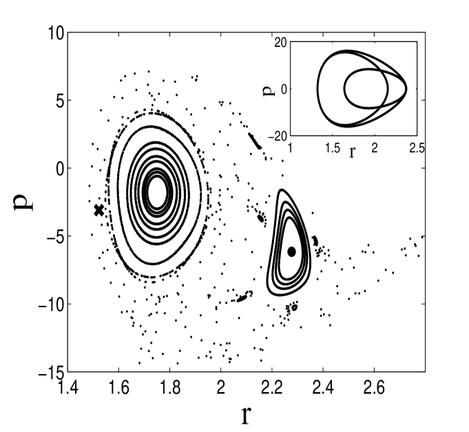
Figure 1: Poincaré section of Hamiltonian (2) for $F_{1}=0.18$, $F_{2}=0.02$ and $\phi=0$. The dot and the cross indicate the elliptic periodic orbit ${\mathcal{O}}_{e}$ and its associated hyperbolic one, respectively. The inset depicts a projection of ${\mathcal{O}}_{e}$ in the $(r,p)$ plane.

Figure 1 shows a Poincaré section (stroboscopic plot of phase space with period $2\pi/\omega_{1}$) of Hamiltonian (2) for amplitudes $F_{1}=0.18$, $F_{2}=0.02$ and phase lag $\phi=0$. We notice that an elliptic island is present at the entrance of the dissociation channel. At the center of this island sits an elliptic periodic orbit with one intersection with the Poincaré surface of section (i.e. with period $2\pi/\omega_{1}$). Standard Hamiltonian dynamics show that the trajectories that are likely to dissociate can become trapped around the resonant island for a while before finding an escape route. Therefore, this particular periodic orbit, which we call ${\mathcal{O}}_{e}$, plays a crucial role in the dissociation probability, and is the focus of the current paper : We investigate its role as the parameters $(F_{1},F_{2},\phi)$ are varied. Due to the symmetry ($\phi\mapsto\pi-\phi$) the fundamental domain of variations of $\phi$ is $[0,\pi[$. We also restrict the amplitudes to $(F_{1},F_{2})\in[0,0.22]\times[0,0.06]$.

We anticipate two factors which can influence dissociation: One is the location of this orbit, and the other is a change of its stability. In Fig. 2, we represented the position of ${\mathcal{O}}_{e}$ or, more precisely, its action and angle variables as defined by gu

$$I=2\left(1-\sqrt{1-E}\right),$$

$$\tan\theta=-\frac{\tilde{p}\sqrt{1-E}}{1-{\rm e}^{-\tilde{r}}-E},$$

where $E(\tilde{r},\tilde{p})=\tilde{p}^{2}+(1-{\rm e}^{-\tilde{r}})^{2}$, for a typical set of parameters $F_{1}=0.18$ and $F_{2}=0.02$, while $\phi$ is varied. The main conclusion is that the variation of the action and angle of ${\mathcal{O}}_{e}$ do not seem to be linked to the variation of the dissociation probability since they do not vary significantly as $\phi$ is increased. In addition they are not monotonic functions of $\phi$ in contrast with the dissociation probability. Hence, the position of the specific periodic orbit does not appear to play a significant role (at least in the range of parameters considered).

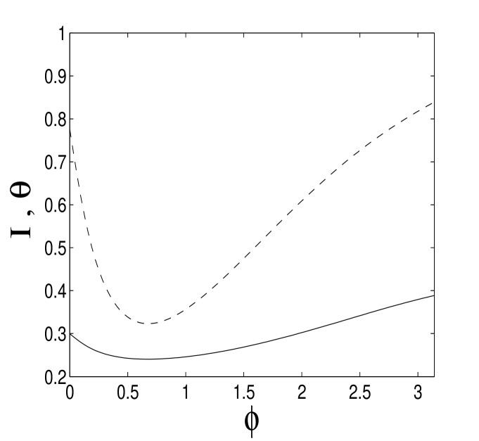
Figure 2: Action(solid) and angle(dashed) curves for $F_{1}=0.18$ and $F_{2}=0.02$.

The second possible mechanism based on a bifurcation has a more drastic influence on dissociation. In order to monitor this bifurcation properly, we also need to follow the associated hyperbolic orbit bach06 . To see an increase of dissociation we need to ensure that the hyperbolic orbit stays hyperbolic while the elliptic one turns hyperbolic (in order to discard a stability exchange which would not affect the dissociation probability significantly). A typical residue plot (the residue as a function of $\phi$) is shown in Fig. 3 for $F_{1}=0.18$ and $F_{2}=0.02$. We notice that an increase of $\phi$ is always associated with an increase of the residue. At $\phi=0.75$, the residue crosses unity and a bifurcation (which is a period doubling) occurs. This increase of hyperbolicity is associated with increased chaos and hence more dissociation. This is in agreement with the direct simulations of Ref. greeks .

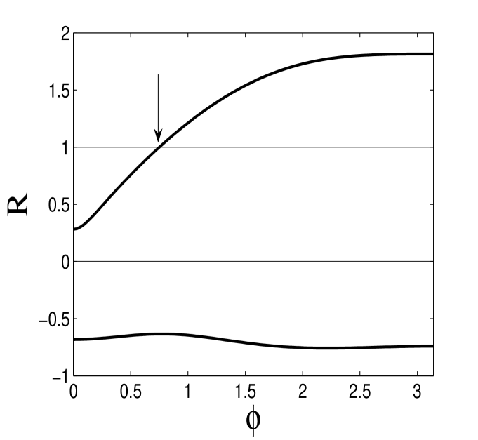
Figure 3: Residue curves (bold solid) for the considered set of periodic orbits for $F_{1}=0.18$ and $F_{2}=0.02$ : for ${\mathcal{O}}_{e}$ (upper curve) and for ${\mathcal{O}}_{h}$ (lower curve). The arrow indicates where the bifurcation happens.

We should point out that the computation of Ref. greeks uses initial conditions in the ground state ($E=0.045$), which is lower than the set of periodic orbits we consider ($E=0.29$) in Fig. 1. This justifies the importance of the chosen periodic orbits for dissociating trajectories. For other values of parameters we consider, the energy level of the periodic orbit ${\mathcal{O}}_{e}$ is always well above $E=0.045$.

IV.2 Residue contour plots in parameter space

For fixed values of $\phi$, we vary the amplitudes $F_{1}$ and $F_{2}$ and compute the residue values of the periodic orbit ${\mathcal{O}}_{e}$. We depict the contour plots of these residues in Fig. 4 in the $(F_{1},F_{2})$ plane for $\phi=0$, $\pi/6$, $\pi/2$ and $\pi$. These figures should be compared to Fig. 2 of Ref. greeks . In Fig. 4, darker regions represent lower residue values, and hence are expected to reveal more stable dynamics ( smaller dissociation probability) for the corresponding parameters.

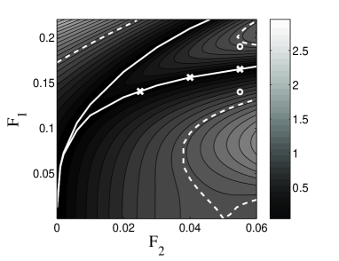
(a)

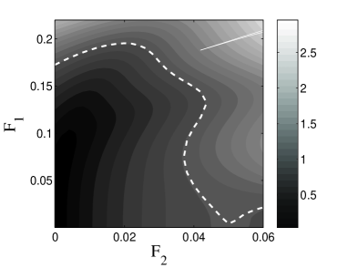
(b)

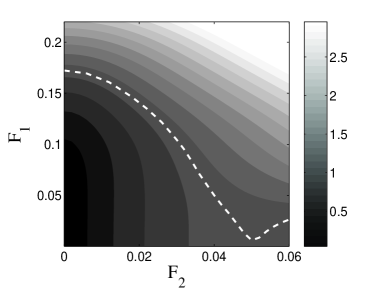
(c)

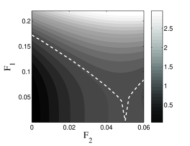
(d)

Figure 4: Contour plots of the residues of ${\mathcal{O}}_{e}$ in the $(F_{1},F_{2})$ plane for $(a)$ $\phi=0$, $(b)$ $\phi=\pi/6$, $(c)$ $\phi=\pi/2$ and $(d)$ $\phi=\pi$. White dashed curves indicate $R(F_{1},F_{2})=1$ where ${\mathcal{O}}_{e}$ bifurcates. Two white solid curves in $(a)$ indicate $R(F_{1},F_{2})=0$. The small region enclosed by two thin white lines near the up-right corner in $(b)$ corresponds to a region where ${\mathcal{O}}_{h}$ is elliptic. Crosses (respectively circles) on panel $(a)$ represent the values of parameters where laminar plots have been computed in Fig. 5 (respectively Fig. 6).

On these residue contours we have superposed the curves $R(F_{1},F_{2})=1$ (white dashed curves) through which the periodic orbit ${\mathcal{O}}_{e}$ changes its stability. The corresponding bifurcation from elliptic to hyperbolic linear stability indicates a possible increase in dissociation probability due to an increase of hyperbolicity in this region of phase space. Since the trajectories are no longer trapped when ${\mathcal{O}}_{e}$ is hyperbolic, it is expected that the dissociation probability increases. This is in good agreement with Ref. greeks where we notice that for $\phi$=$\pi/6$, $\pi/2$ and $\pi$, there is a qualitative agreement in the shape of the dissociation probability. In particular, the following features are reproduced for a fixed value of $\phi$ : the non-monotonicity for $\phi=\pi/6$ as $F_{2}$ is increased (with a fixed value of $F_{1}$), and the monotonicity for $\phi=\pi/2$ and $\pi$ with a sharper downward bifurcation curve (dashed line) for $\phi=\pi$ as $F_{2}$ is increased in the region $F_{2}\in[0,0.05]$. Our analysis also confirms that the stabilization effect decreases when $\phi$ is increased (from 0 to $\pi$). For $\phi=0$ case, the contour plot shows agreement with direct simulations for most regions in the $(F_{1},F_{2})$ plane once more, and the property that it reproduces the two upper-right bumps observed in the dissociation probability contour plot. These are interpreted as remnants of the ellipticity of the bifurcated ${\mathcal{O}}_{e}$. We notice that the corresponding hyperbolic periodic orbit ${\mathcal{O}}_{h}$ remains hyperbolic ($R<0$) for most values of the parameters. However, for $\phi\in[\pi/6,\pi]$, there is a region around the upper-right corner of the $(F_{1},F_{2})$ plane where the ${\mathcal{O}}_{h}$ turns to elliptic and then returns to hyperbolic, as it is shown on the $(F_{1},F_{2})$ plane contour plot of Fig. 4 $(b)$. In general, this bifurcation does not affect the dissociation probability because, due to its location, it does not play an important role compared to the periodic orbit ${\mathcal{O}}_{e}$ which has already bifurcated ($R>1$) for these parameter values (see Figs. 4 $(c)$ and $(d)$). However, for low values of $\phi$ and high values of the amplitudes $F_{i}$, the orbit ${\mathcal{O}}_{e}$ is still elliptic and ${\mathcal{O}}_{h}$ undergoes a bifurcation, as shown in Figs. 7 which we discuss in the following section. This region corresponds to the disagreement observed for $\phi=0$ on Fig. 4 with the direct simulations of Ref. greeks to which we turn next.

IV.3 Low values of $\phi$ : Influence of ${\mathcal{O}}_{h}$

For $\phi=0$, we observe two branches on Fig. 4 $(a)$ where the residues of ${\mathcal{O}}_{e}$ vanish. Along these lines we expect, from a linear stability analysis, locally a constant degree of chaos, and hence dissociation probability. However, this is not seen in direct simulations since the dissociation probability actually increases along these lines as $F_{2}$ is increased. This feature is shown using laminar plots which represent contour plots of the number of return times on the Poincaré section before dissociation (defined as trajectories for which $E$ becomes greater than $E_{th}=2$). The maximum integration time is $200\pi/\omega_{1}\approx 2244$. Figure 5 shows laminar plots for the set of parameters on the line of vanishing residues (as $F_{2}$ is increased) as marked by crosses in Fig. 4 $(a)$, and Figure 6 represents two additional laminar plots for parameter sets transverse to that line (with a fixed $F_{2}$ and increasing $F_{1}$), marked by circles in Fig. 4 $(a)$. These plots show clearly that dissociation increases as $F_{2}$ is increased. Even locally around the considered periodic orbit ${\mathcal{O}}_{e}$, there seems to be more chaos as $F_{2}$ is increased. The situation is more complex at parameter values off the vanishing-residue line as $F_{1}$ is varied on Fig. 6 where the overall amount of dissociation seems to be similar but with very different distributions of dissociating trajectories. All these features originate from the nonlinear stability which can be captured by considering the linear stability of higher order periodic orbits around the boundary of the elliptic island ${\mathcal{O}}_{e}$.

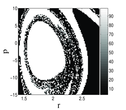
(a)

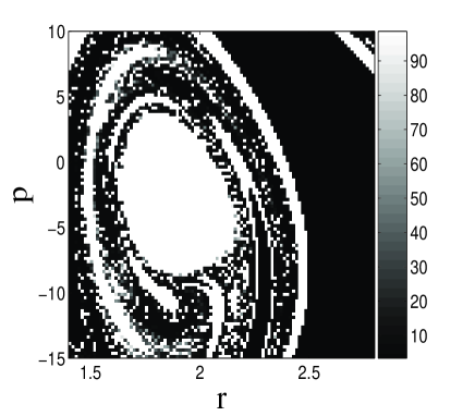
(b)

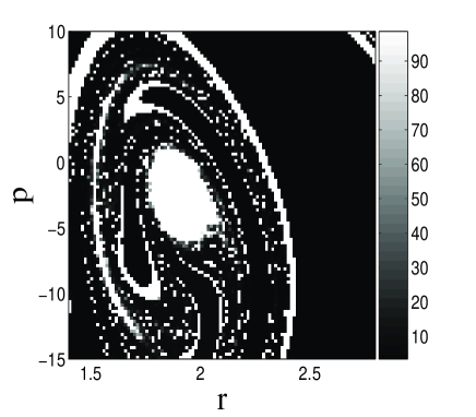
(c)

Figure 5: Laminar plots with $\phi=0$ for $(a)$ $(F_{1},F_{2})=(0.1405,0.025)$, $(b)$ $(F_{1},F_{2})=(0.1559,0.04)$ and $(c)$ $(F_{1},F_{2})=(0.165,0.055)$. The cutoff time is $200\pi/\omega_{1}\approx 2244$ and the energy threshold is $E_{th}=2$.

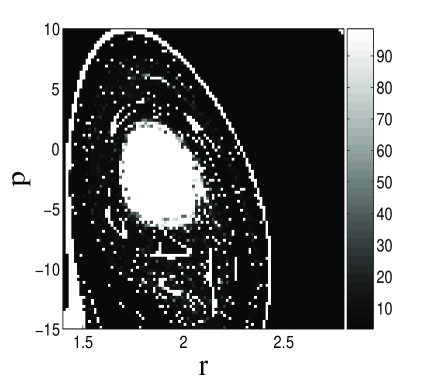
(a)

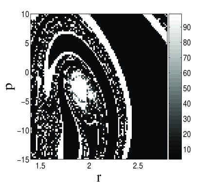
(b)

Figure 6: Laminar plots with $\phi=0$ for $(a)$ $(F_{1},F_{2})=(0.19,0.055)$, and $(b)$ $(F_{1},F_{2})=(0.14,0.055)$. The cutoff time is $200\pi/\omega_{1}\approx 2244$ and the energy threshold is $E_{th}=2$.

For insights into the parameter region where this discrepancy occurs, we describe here the associated bifurcation. In Fig. 7 the residue as a function of $F_{1}$ is plotted for both ${\mathcal{O}}_{e}$ and ${\mathcal{O}}_{h}$ with fixed $F_{2}$ and $\phi$. We see clearly that there is a loop around $R=0$, indicating that ${\mathcal{O}}_{h}$ undergoes a bifurcation at $R=0$ which involves three periodic orbits of the same period, two hyperbolic ones and an elliptic one. When $\phi$ is equal to $0$, the upper part of the loop merges with the residue curve of ${\mathcal{O}}_{e}$, as shown in Fig. 7$(b)$, for which the loop size reaches its maximum size. The following picture emerges : Without a loop in the residue curve, the system has two periodic orbits with the period of the field, ${\mathcal{O}}_{e}$ and ${\mathcal{O}}_{h}$. In the region of parameters where there is a loop in the residues, the system has four of these periodic orbits, two elliptic ones (which are close to each other or even coincide at $\phi=0$) and two hyperbolic ones. This additional hyperbolicity increases chaos (and hence dissociation) locally.

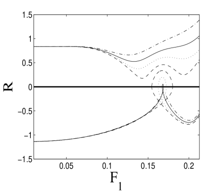
(a)

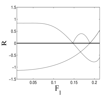
(b)

Figure 7: Residue versus $F_{1}$ for both elliptic and hyperbolic periodic orbits at $F_{2}=0.03$ for $(a)$ several different values of $\phi$ : $\phi=\pi/6$ (dash-dotted), $\phi=0.35$ (solid), $\phi=0.2$ (dotted) and $\phi=0.06$ (dashed), and $(b)$ $\phi=0$.

Conclusions

We have analyzed the dissociation dynamics of a model diatomic molecule driven by a bichromatic field in terms of periodic orbit bifurcations. Following the linear stability of a few selected periodic orbits, we reproduced the dissociation probability qualitatively in parameter space (two field amplitudes and one relative phase). For relatively low $\phi$ and high amplitudes $F_{i}$, the original hyperbolic periodic orbit ${\mathcal{O}}_{h}$ undergoes a particular bifurcation, which leads to two branch lines on the $F_{1}$-$F_{2}$ residue plane. Along these two branch lines, there is a discrepancy between predictions based on the residues and direct simulations. The role of additional periodic orbits is underlined regardless of whether the discrepancy originates from bifurcated orbits (and the resulted increase of hyperbolicity) or from higher-order periodic ones.

References

- (1) M. Shapiro and P. Brumer, Rep. Prog. Phys. 66, 859 (2003).
- (2) R. J. Gordon, L. Zhu and T. Seideman, Acc. Chem. Res. 32, 1007 (1999).
- (3) V. S. Batista and P. Brumer, Phys. Rev. Lett. 89, 143201 (2002).
- (4) E. Charron, A. Giusti-Suzor and F. H. Mies, Phys. Rev. A 49, R641 (1994).
- (5) M. E. Goggin and P. W. Milonni, Phys. Rev. A 38, 5174 (1988).
- (6) J. R. Stine and D. W. Noid, Opt. Commun. 31, 161 (1979).
- (7) V. Constantoudis and C. A. Nicolaides, J. Chem. Phys. 122, 084118 (2005).
- (8) J. Levesque, S. Chelkowski and A. D. Bandrauk, J. Phys. Chem. A 107, 3457 (2003).
- (9) F. He, C. Ruiz and A. Becker, Phys. Rev. Lett. 99, 083002 (2007).
- (10) Y. Gu and J.-M. Yuan, Phys. Rev. A 36, 3788 (1987).
- (11) V. Constantoudis and C. A. Nicolaides, Phys. Rev. E 64, 056211 (2001).
- (12) V. Constantoudis and C. A. Nicolaides, Phys. Rev. A 55, 1325 (1997).
- (13) M. E. Goggin and P.W. Milonni, Phys. Rev. A 37, 796 (1988).
- (14) A. Guldberg and G. D. Billing, Chem. Phys. Lett. 186, 229 (1991).
- (15) B. Wu and W-K. Liu, Physica A 205, 470 (1994).
- (16) M. Thachuk and D. M. Wardlaw, J. Chem. Phys. 102, 7462 (1995).
- (17) C. A. Nicolaides, Th. Mercouris and I. D. Petsalakis, Chem. Phys. Lett. 212, 685 (1993).
- (18) P. C. Dardi and S. K. Gray, J. Chem. Phys. 77, 1345 (1982).
- (19) R. Heather and H. Metiu, J. Chem. Phys. 88, 5496 (1988).
- (20) A. D. Bandrauk, E-W. S. Sedik and C. F. Matta, J. Chem. Phys. 121, 7764 (2004).
- (21) S. Huang, C. Chandre and T. Uzer, J. Phys. B 40, F181 (2007); J. Phys. B 41, 035604 (2008).
- (22) R. Bachelard, C. Chandre and X. Leoncini, Chaos 16, 023104 (2006).
- (23) M. Joyeux, S. Yu. Grebenshchikov, J. Bredenbeck, R. Schinke and S. C. Farantos, Adv. Chem. Phys. 130, 267 (2005).
- (24) S. C. Farantos, Z.W. Qu, H. Zhu and R. Schinke, Int. J. Bifurcation Chaos Appl. Sci. Eng. 16, 1913 (2006).
- (25) P. Cvitanović, R. Artuso, R. Mainieri, G. Tanner and G. Vattay, Chaos: Classical and Quantum, ChaosBook.org (Niels Bohr Institute, Copenhagen 2005).
- (26) J. M. Greene, J. Math. Phys. 20, 1173 (1979).
-
(27)
R. S. MacKay, Nonlinearity 5, 161 (1992).