When are recommender systems useful?

Abstract

Recommender systems are crucial tools to overcome the information overload brought about by the Internet. Rigorous tests are needed to establish to what extent sophisticated methods can improve the quality of the predictions. Here we analyse a refined correlation-based collaborative filtering algorithm and compare it with a novel spectral method for recommending. We test them on two databases that bear different statistical properties (MovieLens and Jester) without filtering out the less active users and ordering the opinions in time, whenever possible. We find that, when the distribution of user-user correlations is narrow, simple averages work nearly as well as advanced methods. Recommender systems can, on the other hand, exploit a great deal of additional information in systems where external influence is negligible and peoples’ tastes emerge entirely. These findings are validated by simulations with artificially generated data.

1 Introduction

One of the most amazing trends of today’s globalized economy is peer production [Anderson (2006)]. An unprecedented mass of unpaid workers is contributing to the growth of the World Wide Web: some build entire pages, some only drop casual comments, having no other reward than reputation [Masum and Zhang (2004)]. Many successful websites (e.g. Blogger and MySpace) are just platforms holding user-generated content. The information thus conveyed is particularly valuable because it contains personal opinions, with no specific corporate interest. It is, at the same time, very hard to go through it and judge its degree of reliability. If you want to use it, you need to filter this information, select what is relevant and aggregate it; you need to reduce the information overload [Maes (1994)].

As a matter of fact, opinion filtering has become rather common on the web. There exist search engines (e.g. Googlenews) that are able to extract news from journals, websites (e.g. Digg) that harvest them from blogs, platforms (e.g. Epinions) that collect and aggregate votes on products. The basic version of these systems ranks the objects once for all, assuming they have an intrinsic value, independent of the personal taste of the demander [Laureti et al. (2006)]. They lack personalisation [Kelleher (2006)], which constitutes the new frontier of online services.

Users need only browse the web in order to leave recorded traces, the eventual comments they drop add on to it. The more information you release, the better the service you receive. Personal information can, in fact, be exploited by recommender systems. The deal becomes, at the same time, beneficial to the community, as every piece of information can potentially improve the filtering procedures. Amazon.com, for instance, uses one’s purchase history to provide individual suggestions. If you have bought a physics book, Amazon recommends you other physics books: this is called item-based recommendation [Breese et al. (1998), Sarwar et al. (2001)]. Those who have experience with it know that this system works fairly well, but it is conservative as it rarely dares suggesting books regarding subjects you have never explored. We believe a good recommender system should sometimes help uncovering people’s hidden wants [Maslov and Zhang (2001)].

Collaborative filtering is currently the most successful implementation of recommendation systems. It essentially consists in recommending you items that users, whose tastes are similar to yours, have liked. In order to do that, one needs collecting taste information from many users and define a measure of similarity. The easiest and most common ways to do it is to use either correlations or Euclidean distances.

Here we test a correlation-based algorithm and a spectral method to make predictions. We describe these two families of recommender systems in section 2, and propose some improvements to currently used algorithms. In section 3 we present the results of our predicting methods on the MovieLens and Jester data sets, as well as on artificial data. We argue that the distribution of correlations in the system is the key ingredient to state whether or not sophisticated recommendations outperform simple averages. Finally, we draw some conclusions in section 4.

2 Methods

Our aim is here to test two methods for recommending, spectral and correlation-based, on different data sets. The starting point is data collection. One typically has a system of $N$ users, $M$ items and $n$ evaluations. Opinions, books, restaurants or any other object can be treated, although we shall examine in detail two fundamentally different examples: movies and jokes. Each user $i$ evaluates a pool of $n_{i}$ items and each item $\alpha$ receives $n_{\alpha}$ evaluations, with $n=\sum_{i=1}^{N}n_{i}=\sum_{\alpha=1}^{M}n_{\alpha}$. The votes $v_{i\alpha}$ can be gathered in a matrix $V$. If a user $j$ has not voted on item $\beta$, the corresponding matrix element takes a constant value $v_{j\beta}=$ EMPTY, usually set to zero.

Once the data collected into the voting matrix, we aim to predicting votes before they are expressed. That is, we would like to predict if agent $j$ would appreciate the movie, book or food $\beta$, before she actually watched, read or ate it. Say, we predict that user $j$ would give a very high vote to item $\beta$ if she were exposed to it; we can then recommend $\beta$ to $j$ and verify a posteriori her appreciation. Ideally, we would like to have a prediction for every EMPTY element of $V$.

Most websites only allow votes to be chosen from a finite set of values. In order to take into account the fact that each person adopts an individual scale, we compute each user’s $i$ average expressed vote $\left\langle{v_{i}}\right\rangle$ and subtract it from non empty $v_{i\alpha}$’s. The methods we analyze give predictions in the following form [Delgado (1999)]:

$$v_{j\beta}^{\prime}=\left\langle{v_{j}}\right\rangle+\sum_{i=1}^{N}S_{ji}(v_{i\beta}-\left\langle{v_{i}}\right\rangle),$$ (1)

where $v_{j\beta}^{\prime}$ is the predicted vote and $S$ is a similarity matrix. The choice of $S$ is the crucial issue of collaborative filtering. One has, in fact, very often to face a lack of data, which makes it difficult to estimate the similarity between non overlapping users. We shall describe, in the following, correlation-based and spectral techniques to cope with this problem.

2.1 Correlation

Correlation-based methods for recommending make use of user-user linear correlations as similarity measures. If we call $\left\langle{v_{i}}\right\rangle$ the average vote expressed by user $i$, the correlations $C_{ij}$ can be calculated with Pearson’s formula [Press et al. (1992)]:

$$C_{ij}={{\sum_{\alpha}(v_{i\alpha}-\left\langle{v_{i}}\right\rangle)(v_{j\alpha}-\left\langle{v_{j}}\right\rangle)}\over{\sqrt{\sum_{\alpha}(v_{i\alpha}-\left\langle{v_{i}}\right\rangle)^{2}}\sqrt{\sum_{\alpha}(v_{j\alpha}-\left\langle{v_{j}}\right\rangle)^{2}}}},$$ (2)

with $C_{ij}=0$ if users $i$ and $j$ haven’t judged more than one item in common. Unexpressed votes can then be forecast by setting $S_{ij}\propto C_{ij}$ in eq. (1). This estimation is often used as a rule of thumb, without knowing if it is justified and why. There is, at our knowledge, only one model [Bagnoli et al. (2003)] where the convergence of $v_{j\beta}^{\prime}$ to the real vote, in the limit of an infinite system, is guaranteed.

The use of pair correlations alone is often not very effective in predicting tastes. In fact, $C_{ij}$ is a measure of similarity between the behavior of two users who have expressed votes on a number $n_{ij}$ of commonly evaluated items. When the matrix $V$ is very sparse and $n_{ij}$, as a consequence, small or zero for many couples of users, such a measure becomes poorly informative. A popular solution to this problem [Blattner et al. (2007)] is to estimate unknown votes via a linear combination of $v_{j\beta}^{\prime}$ and a global average, i.e. $v_{j\beta}^{\prime\prime}\propto qv_{j\beta}^{\prime}+(1-q)m(\beta),$ where $q$ is a constant weight between $0$ and $1$ and $m(\beta)$ the average vote expressed on item $\beta$ by all users. The typical choice, $q=1/2$, amounts to defining $S_{ij}=1/n_{\beta}+C_{ij}$ in eq. (1).

After testing many different versions of correlation-based recommendations, with the same number of free parameters, we chose a more effective ansatz: every time $C_{ij}=0$ we replace it with the average value of the correlation across the population. Such a mean-field solution improves the results and eliminates, at the same time, the parameter $q$. As for the normalization of the weighted sum in eq. (1), we found that the best choice is $S_{ji}=C_{ji}/\sum_{i}|C_{ji}|$. Small adjustments can be made on the minimal number of common items $n_{c}$ required to compute correlations. A low value of $n_{c}$ may, in fact, improve the average prediction quality at the price of very large fluctuations. We set $n_{c}=3$ in most cases.

Let us stress here that the method we used can be further improved by calibrating additional parameters. Case amplification [Breese et al. (1998)], for instance, consists in taking a similarity measure proportional to some power $\gamma$ of the correlation, in order to punish low correlation values. Upon optimizing the value of $\gamma$, the prediction power of our correlation-based method is able to compete with that of spectral techniques [Moret (2007)].

2.2 Spectral

An alternative approach to recommending makes use of spectral techniques [Sarwar et al. (2000), Billsus and Pazzani (1998)]. Users can be represented by their vectors of votes $\vec{v}_{i}$ in a $M$-dimensional metric space $\mathcal{M}$. One can define, between all couples of users $(i,j)$, an overlap $\Omega_{ij}$ as a decreasing function of their distance. Users can thus be represented as nodes of a weighted graph. Spectral methods have recently been used to detect clusters in networks [Seary and Richards (2003), Donetti and Munoz (2004), Capocci et al. (2005)] and can equally be applied to devise recommender systems. In order to implement them for this purpose, we take the following fundamental steps: i) Calculate the overlap matrix $\Omega$ that defines our weighted graph. ii) Find the spectrum of its Laplacian after dimensionality reduction. iii) Calculate user similarities using eigenvectors’ elements, and make predictions with eq. (1). The method is not trivial and each one of the preceding points contains subtleties. After testing many different options, we have used the one that yields the best and more stable results.

The definitions and the procedures we shall describe here, stand on the following assumption: if we disposed of the votes of all users on all items, the points of coordinates $\vec{v}_{i}$ would only occupy a compact subspace of $\mathcal{M}$, a manifold-like structure of dimension $k<<M$. This approach, whose validity will be verified a posteriori, is inspired by ref. [Belkin and Niyogi (2003)], where the interested reader can find the details.

A preliminary step is the substitution of the EMPTY entries of the voting matrix with the corresponding object’s average received vote $m(\alpha)$. We then define the elements of the overlap matrix as $\Omega_{ij}=\exp(-d_{ij}^{2}/\Gamma^{2})$, where $d_{ij}=||\vec{v}_{i}-\vec{v}_{j}||$ is the Euclidian distance between the vectors of votes of users $i$ and $j$. $\Omega$ gives higher weights to pairs of users whose votes are closer, and reaches its maximum $\Omega_{ij}=1$ when the distance is $0$. The external parameter $\Gamma^{2}$ controls the size of the neighborhood, since $\Omega_{ij}\to 0$ for $d_{ij}\gg\Gamma$. The performance of our experiments was almost unchanged within a wide range of this parameter. We fixed $\Gamma=\max_{i,j}d_{ij}$, which allows to develop the exponential $\exp(-d^{2}/\Gamma^{2})\simeq 1-(d/\Gamma)^{2}$. Hence we set

$$\Omega_{ij}=1-\left(\frac{||\vec{v}_{i}-\vec{v}_{j}||}{\max_{i,j}||\vec{v}_{i}-\vec{v}_{j}||}\right)^{2}.$$

In order to obtain the optimal embedding in $k$ dimensions of the structure formed by users in the space of the votes, ref. [Belkin and Niyogi (2003)] prescribes to find the first $k$ eigenvectors of the normalized Laplacian $L=D^{-1/2}(D-\Omega)D^{-1/2}$ of $\Omega$, where $D$ is its diagonal weight matrix, of elements $D_{ii}=\sum_{j}\Omega_{ij}$. When used for partitioning the population of users, the spectrum of the normalized Laplacian $L$ has revealed more effective and stable than that of other matrices [von Luxburg et al. (2004)]. Let $\vec{y}_{0},.....,\vec{y}_{k-1}$ be its first $k$ eigenvectors, in order of increasing eigenvalues. Note that $\vec{y}_{0}$ always has eigenvalue $0$. The other non-trivial eigenvectors contain information about eventual subgraphs [Seary and Richards (2003)]. If the graph is connectected and bipartite, for instance, the components of $\vec{y}_{1}$ will be positive for one subgraph and negative for the other. Whenever the two subgraphs are not very well separated, the distinction between the two components becomes progressively fuzzier. An example is given by the left graph of fig. 1, where the components $y_{1}(j),j=1,2,...,N$ of the first non-trivial eigenvector of the Laplacian of the Jester database show a clear discontinuity. Higher eigenvectors contribute to define the first two clusters and can reveal the contours of more weakly connected blocks [Simonsen et al. (2003)]. The right graph of fig. 1, in fact, shows the projection of the Jester matrix on the first two non-trivial eigenvectors. The presence of two islands can be detected by eye inspection, confirming that Jester users can be grouped in, at least, two different categories.

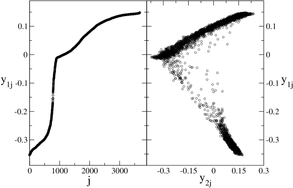
Figure 1: Identification of clusters of users in Jester with spectral analysis. Left graph: $10\times$value of the elements of the first non-trivial eigenvector $\vec{y}_{1}$ of the normalized Laplacian matrix, plotted against their cardinality. The clear discontinuity around $0$ indicates the presence of two big clusters. Right graph: The first non-trivial eigenvector is plotted here against the second. The presence of the two main clusters is clearly visible.

Let us now come back to the application of our spectral analysis to recommending systems. Each user $i$ can be represented by a point in the $(k-1)$-dimensional subspace made of the $i$th components of the first $k$ eigenvectors, i.e. $\vec{y}(i)=({y}_{1}(i),...,{y}_{k-1}(i))$. One can think that each one of these coordinates contains information about the degree of participation of user $i$ in a subgroup of users. The parameter $k$, which plays the key role in dimensionality reduction, has to be determined by a cross checking procedure: we measure the performance of the algorithm on the training set for different values of $k$, and choose the one which supplies the best results. In our experiments this is of order $10$.

Finally, we calculate the similarity $S_{ij}$ for each pair of users. After comparing many different measures, the cosine turned out to work best. Thus we define

$$S_{ij}=\frac{\vec{y}(i)^{T}\vec{y}(j)}{||\vec{y}(i)||||\vec{y}(j)||},$$

where the superscript $T$ denotes the transposed of a vector, and $||\cdot||$ is the ordinary $L_{2}$ norm. Here $S_{ij}$ can be interpreted as an overlap between the participation ratio of two users to different groups of taste. Armed with this similarity matrix, we predict votes according to eq. (1). Our spectral technique, although very tedious, performs better than the other methods we tested.

3 Experiments

The purpose of this paper is to evaluate different collaborative filtering algorithms, and to establish when they can be used effectively. To this end, we have tested the methods described above on two data sets, carrying completely different features: MovieLens and Jester. In order to achieve a better understanding of the role played by correlations in the votes, we have also made simulations on artificially generated data. Prior to presenting our results, we shall describe the data sets used for the experiment.

3.1 Data sets

MovieLens (movielens.umn.edu) is a webservice of the GroupLens project (grouplens.org),that recommends movies. Users ratings are recorded on a five stars scale and contain additional information, such as the time at which an evaluation has been made. The data set we downloaded contains $6040$ users $\times$ $3952$ movies, where only a fraction $\eta_{M}=0.041$ of all possible votes has actually been expressed. Jester (shadow.ieor.berkeley.edu/humor)is an online joke recommendation system. It contains $73421$ users $\times$ $100$ jokes and a fraction $\eta_{J}=0.55$ of expressed votes. Users ratings are real numbers ranging from $-10$ to $10$.

While both websites collect ratings of users on items, they differ substantially in many respects: the range of allowed ratings $R$, the users-to-items ratio $N/M$, the sparsity of the voting matrix and the distribution of votes, among others. In fact, while the MovieLens data set is roughly symmetric, the Jester one is heavily asymmetric, with users outnumbering items by a factor $734$. This is because of the fixed, low number of jokes ($M_{J}=100$) one can evaluate in Jester. For the same reason, the MoviLens data set is much sparser than Jester. In fact, defining the sparsity coefficient as $\eta=n/(M\times N)$, where $n$ is the number of recorded ratings, one has $\eta_{M}\simeq 4\%$ and $\eta_{J}\simeq 55\%$. Note that $\eta$ decreases as the matrix gets sparser, and not vice versa.

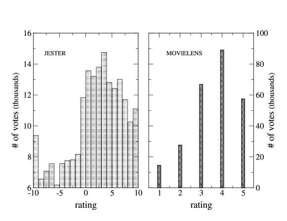
Figure 2: Distribution of votes for Movielens and Jester.

The most fundamental difference, though, is the amount of a priori information provided to users. People choose the movies they want to watch on the basis of a preliminary selection. They know actors and directors, read reviews and are exposed to advertisements. When they actually buy the entrance ticket, they have some motivated expectactions. Accordingly, in the MovieLens data set, the distribution of all the issued votes is unimodal and noticeably shifted towards the positive region (see fig. 2, right panel). No preselection, on the other hand, is possible with online jokes, giving rise to a more uniform distribution of votes. This can be verified by arranging the votes on a $5$ beans histogram and computing the entropy $S=-\sum_{i}p_{i}\log_{5}p_{i}$, which yields $S_{J}=0.98$ for Jester and $S_{M}=0.90$ for MovieLens. In addition to that, the distribution of votes is slightly bimodal in Jester, as shown in the left panel of fig. 2. This suggests the existence of groups of users with similar taste, which is confirmed by fig. 1, as already pointed out. In order to gain more insight into this fundamental difference, we also report, in fig. 5, the distribution of user-user correlations, the effects of which will be discussed in section 3.4.

The size of the data sets has been reduced by roughly $50$% in both dimensions. As the cancellations have been done randomly, the statistical properties of the original data have been preserved. In particular, we tried to maintain the probability distribution of the number of votes per users, as well as the sparsity and the $N/M$ ratio. We want to stress that this is crucial when testing the performance of predictive algorithms on real data in an objective way. In fact, many experiments can be found in the literature that only test recommender systems on dense voting matrices. Typically, users who have judged too few items are struck out, as well as items that have received too few votes. We did not comply to such an habit and made an effort to keep the filtering level as low as possible, although this makes predictions much more difficult.

Once filtered, the data are divided into a training and a test set. The training set is composed of the data one actually uses to make predictions on the missing evaluations contained in the test set. This last is only employed afterwards, to compare predictions and realised evaluations. We have chosen test sets of dimension $n_{test}=10^{4}$ for both databases. The experiments have been carried out as follows. First, we fix the test set and never change it through the simulation. Then we progressively fill the training set over time and make predictions on the entire test set at fixed time steps.

Many different accuracy metrics have been proposed to assess the quality of recommendations (see ref. [Herlocker et al. (2004)]), one of the most common of which being the Mean Average Error:

$$MAE=\frac{1}{n_{test}R}\sum_{j,\beta}|v_{j\beta}^{\prime}-v_{j\beta}|,$$ (3)

where the sum runs over all expressed votes in the test set and $R=|v_{max}-v_{min}|$ is the size of the domain of all possible ratings. In our experiments, the MAE is calculated, at different sparsity values $\eta$, on a unique test set. The results for our sets of data will be presented in the following sections.

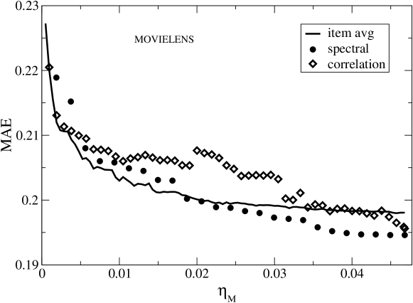
Figure 3: MAE of spectral (with $k=20$), correlation-based methods and movie average $m(\alpha)$, as a function of $\eta_{M}$, for the Movielens reduced data set ${V}_{M}$. The sparsity coefficient $\eta_{M}$ is increased according to the timestamps of the expressed votes. The test set is composed by the last $10^{4}$ evaluations.

3.2 MovieLens

After the filtering procedure, we cast the data set in a voting matrix $V_{M}(N\times M)$, with $N=3020$ and $M=1976$. As previously mentioned, the MovieLens database contains the time at which evaluations have been made. We have sorted the votes according to their relative timestamp, both in the training set ${V}_{M}$ and in the test set, which is composed of the last $10^{4}$ expressed votes. Such a choice is intended to reproduce real application tasks, where one aims to predict future votes –which is, of course, much harder than predicting randomly picked evaluations. It is somewhat less realistic to fix the test set once for all, but this has the advantage to allow for more objective comparisons of the results.

The training set has been filled, as well, by adding one vote at a time, according to the temporal ordering. Predictions have been made at fixed sparsity values, as shown in fig. 3. The MAE obtained with spectral and correlation-based methods are compared therein. The solid line is the MAE of predictions made by taking the average vote received by each movie $m(\alpha)$. Surprisingly, the results achieved with this naive estimator are comparable to those of the sophisticated methods, and outperform them in the very sparse region. Note that the movie average predicts the same vote for every user, while the other methods produce personalized recommendations. Their utility only emerges after a crossover value $\eta_{M}\simeq 0.5$. For most fillings, our spectral method (diamonds) performs slightly better than our correlation method (circles), which also suffers of stronger fluctuations.

3.3 Jester

After reduction, we are left with a data set that can be cast in a voting matrix $V_{J}(N\times M)$, with $N=3671$ and $M=100$. The test set has been fixed once for all by random choice of $10^{4}$ evaluations. The training set has been filled randomly and predictions have been produced at increasing $\eta$ values. The results are shown in fig. 4. While in the MovieLens data set the item’s average received vote $m(\alpha)$ is a good predictor for all users, here it is not at all the case. A much better estimate can be produced by the average vote a user has given to any item, represented by the straight line in fig. 4. In fact, in this case, votes are given on an individual basis: both the absolute opinions and the rating scales differ severely from user to user. This might partly explain the fact that sophisticated methods enjoy an edge over simple averages. Our spectral method (squares) performs much better than our correlation method (circles), which, in turn, beats the user average $\left\langle{v_{i}}\right\rangle$ by a large amount.

All methods give rise to a smaller error in the Jester than in the MovieLens set. This is due to various factors. First, $V_{M}$ is sparser than $V_{J}$. Comparing the predictions at the same level of sparsity, though, Jester remains more predictable (with our spectral method), in spite of the much smaller size of its data set. A second factor is represented by the choice of the test set, which is not random in the MovieLens case. Finally, the average correlation of Jester users is higher than that of MovieLens. A more detailed explanation needs an analysis of the entire distribution of correlations, which is the object of the next section.

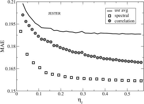
Figure 4: MAE of spectral (with $k=8$), correlation-based methods and user average $\left\langle{v_{i}}\right\rangle$, as a function of the sparsity, for the Jester data set ${V}_{J}$. Here $\eta_{J}$ is increased by random addition of votes. The test set contains $10^{4}$ randomly picked evaluations.

3.4 Simulations

The performance of any recommender system depends on the structure of the data set under investigation. Upon assuming that the user-user correlation is the relevant variable, the shape of its distribution can give us some preliminary information. Since correlations are a measure of similarity of people’s tastes, it is trivial to understand that, when all users are equally correlated, the item’s average received vote is the best predictor. When the distribution of correlations is broad, on the other hand, it becomes useful to make individual predictions, giving more weight to highly correlated mates. For simplicity, the analysis can be restricted to the mean and the standard deviation of the distribution of correlations. A higher absolute mean increases the predictability; a broader distribution enriches the information encoded and requires clever methods to be exploited.

As a preliminary check of our analysis, we can look at the user-user correlations, as calculated from eq. (2), of our two data sets. It is evident from fig. 5 that Jester has a higher mean correlation ($\mu_{J}\simeq 0.1$) than MovieLens ($\mu_{M}\simeq 0.02$), in accordance with the fact that Jester allows for better predictions. It also appears that Movielens correlations have a lower standard deviation ($\sigma_{J}\simeq 0.16$ vs. $\sigma_{M}\simeq 0.05$). This explains, in our framework, why sophysticated methods give much better results than simple averages in Jester (see fig. 4) and not in the case of MovieLens (see fig. 3).

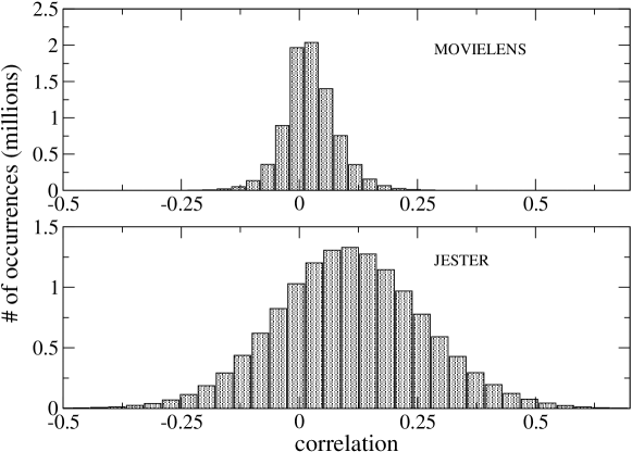
Figure 5: Distribution of correlations for Movielens and Jester.

To test our hypothesis in a systematic way, we generate artificial votes, where we control the structure of the correlation distribution, according to the following procedure. First, we create a valid correlation matrix $\bar{C}$ of fixed size $N\times N$, with the desired mean $\mu$ and variance $\sigma^{2}$, as explained in appendix A. Then we draw a multivariate Gaussian distribution of votes $\bar{V}(N\times M)$, with $\bar{C}$ as input correlation matrix. Finally, we perform predictions on these artificially generated data, comparing our correlation-based method with simple averages.

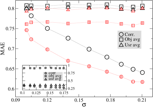
Figure 6: Main graph: Mean prediction error of three recommending methods (user average, item average, correlation-based), as a function of the standard deviation $\sigma$ of user-user correlations. The dimension of the data set, generated artificially as in section 3.4, is $N=250$, $M=500$. The correlation matrix is distributed uniformly, with mean $\mu=0$ (empty symbols) and $\mu=0.1$ (filled symbols). The lines are only meant to guide the eye. Inset: Same as the main graph, with $\mu=0.1$, but here the votes follow a bimodal distribution. As a consequence, the user average $\left\langle{v_{i}}\right\rangle$ works better than the item average $m(\alpha)$.

In fig. 6 we plot, for two different values of $\mu$, the MAE of the predictions as a function of $\sigma$. In the main graph, open and filled symbols are simulations performed with $\mu=0$ and $\mu=0.1$ respectively. As expected, the performance of user averages $\left\langle{v_{i}}\right\rangle$, represented by triangles, does not depend on the parameters of the distribution of correlations –as long as the distribution of votes is unimodal. On the contrary the object average $m(\alpha)$, represented by squares, obviously improves when $\mu$ increases, but it is still independent of $\sigma$. The correlation method also works better for $\mu=0.1$ (filled circles) than for $\mu=0$ (empty circles). Its MAE diminishes as well for increasing $\sigma$. When $\sigma$ goes to zero, in fact, all pair correlations are equal $C_{ij}=c\quad\forall i,j$ and the correlation-weighted sums in eq. (1) become proportional to $m(\alpha)$. This appears clearly in fig. 6, where circles and squares tend to overlap for $\sigma\to 0$. A similar situation occurs in the MovieLens database, where both $\mu$ and $\sigma$ are very small. It is not surprising that, in the sparse region of fig. 3, the mean becomes an even better predictor.

Votes in the Jester database can be better predicted by user averages $\left\langle{v_{i}}\right\rangle$ than by item averages $m(\alpha)$. The reason for this is that users are grouped, as shown in fig. 1. The distribution of Jester votes is, as appears in fig. (2), slightly bimodal. We have generated a data set with this additional feature and plotted the result in the inset of fig. 6. We obtain a behaviour that is similar to that of fig. 4, confirming our hypothesis.

4 Conclusions

We have introduced a new method for recommending, based on the spectrum of the normalized Laplacian of a weighted graph in the user space. This has been tested on the MovieLens and Jester databases, together with a refined correlation-based method.

The experiments have been made on raw data, without altering the statistical properties of the original voting matrix. In particular, no restriction has been imposed on the minimal number of votes expressed by users or received by items. For Movielens, the opinions have been ordered according to their timestamp.

Our spectral method proves to be the most effective in all cases considered. The predictive power of recommender systems is stronger in the Jester than in the MovieLens case, where simple averages are able to detect most information contained in the data. We argue that this phenomenon is due, at least in part, to a different distribution of user-user correlations. When the latter is broader, in fact, sophisticated methods are much more rewarding. A distinction between unimodal and bimodal distributions of votes has been made to determine the best way to take simple averages.

In conclusion, our findings can be used to determine whether or not it is worth to develop complex methods for recommending in specific contexts.

Appendix A How to draw a valid correlation matrix

Here we explain the procedure, inspired by ref. [Jaeckel and Rebonato (2000)], to create the correlation matrix $\bar{C}$ used to draw a multivariate Gaussian distribution of votes. The pair correlation of the population of users must follow a given distribution with the desired mean $\mu$ and variance $\sigma$. Moreover, the matrix we are looking for must be positive semi-definite, i.e. $\lambda_{i}\geq 0\quad\forall i$, where the $\lambda_{i}$’s are the eigenvalues of $\bar{C}$. Let us construct it step by step.

I) We create a square matrix $A(N\times N)$, with elements $A_{ij}$ drawn from a given distribution (uniform in our simulations) of mean $\mu$ and variance $\sigma$. $A$ will not be symmetric in general. II) We apply the transformation $\bar{A}=U+U^{T}$, where $U$ is the upper triangular matrix of $A$ and $U^{T}$ its transposed. $\bar{A}$ is now symmetric, but not positive semi-definite. III) We calculate the right eigensystem $E$ of the real symmetric matrix $\bar{A}$ and its associated set of eigenvalues $\{\lambda_{i}\}$. Hence $\bar{A}\cdot C=\Lambda\cdot E$, with $\Lambda=diag(\lambda_{i})$. Some eigenvalues can be netative. IV) Let us define $\lambda^{{}^{\prime}}_{i}=\lambda_{i}\quad\forall\lambda_{i}>0$, $\lambda^{{}^{\prime}}_{i}=0$ otherwise. The diagonal matrix $\Lambda^{\prime}$ has then semi-positive elements $\lambda^{{}^{\prime}}_{i}$. V) Given the scaling matrix $T_{i}=\left[\sum_{m}s_{im}^{2}\lambda^{{}^{\prime}}_{m}\right]^{-1}$ and the matrices $B^{\prime}=E\sqrt{\Lambda^{\prime}}$ and $B=\sqrt{T}E\sqrt{\Lambda^{\prime}}$, the matrix $\bar{C}=BB^{T}$ is positive-semidefinite and has unit diagonal elements by contstruction, but not the desired mean and variance we imposed on the original matrix $A$. VI) By adding a constant value to the elements of $\bar{C}$, we adjust its mean to $\mu$ and its standard deviation to $\sigma$. We rename the matrix thus obtained $\bar{A}$ and iterate the algorithm, from step III, till the good values of $\mu$ and $\sigma$ are obtained for $\bar{C}$ with the desired precision.

The authors would like to aknowledge the inspiring guide of Yi-Cheng Zhang, as well as the useful discussions they had with Lionel Moret and Hassan Masum. This work has been supported by the Swiss National Science Foundation under grant number 205120-113842.

References

- Anderson (2006) Anderson, C. 2006. People power. Wired News 14, 07.
- Bagnoli et al. (2003) Bagnoli, F., Berrones, A., and Franci, F. 2003. De gustibus disputandum - forecasting opinions from knowledge networks. Physica A 332, 509–518.
- Belkin and Niyogi (2003) Belkin, M. and Niyogi, P. 2003. Laplacian eigenmaps for dimensionality reduction and data representation. Neural Comput. 15, 6, 1373–1396.
- Billsus and Pazzani (1998) Billsus, D. and Pazzani, M. 1998. Learning collaborative information filters. Proc. Int’l Conf. Machine Learning.
- Blattner et al. (2007) Blattner, M., Zhang, Y., and Maslov, S. 2007. Exploring an opinion network for taste prediction: An empirical study. Physica A 373, 753–758.
- Breese et al. (1998) Breese, J., Heckerman, D., and Kadie, C. 1998. Empirical analysis of predictive algorithms for collaborative filtering. In Proceedings of the 14th Annual Conference on Uncertainty in Artificial Intelligence (UAI-98). Morgan Kaufmann, San Francisco, CA, 43–52.
- Capocci et al. (2005) Capocci, A., Servedio, V., Caldarelli, G., and Colaiori, F. 2005. Detecting communities in large networks. Physica A 352, 669–676.
- Delgado (1999) Delgado, J. 1999. Memory-based weightedmajority prediction for recommender systems.
- Donetti and Munoz (2004) Donetti, L. and Munoz, M. 2004. Detecting network communities: a new systematic and efficient algorithm. J. Stat. Mech. P10012.
- Herlocker et al. (2004) Herlocker, J., Konstan, J., Terveen, L., and Riedl, J. 2004. Evaluating collaborative filtering recommender systems. ACM Trans. Inf. Syst. 22, 1, 5–53.
- Jaeckel and Rebonato (2000) Jaeckel, P. and Rebonato, R. 1999/2000. The most general methodology for creating a valid correlation matrix for risk management and option pricing purposes. Journal of risk 2, 2.
- Kelleher (2006) Kelleher, K. 2006. Personalize it. Wired News 14, 07.
- Laureti et al. (2006) Laureti, P., Moret, L., and Zhang, Y. 2006. Information filtering via iterative refinement. Europhysics Letters 75, 1006.
- Maes (1994) Maes, P. 1994. Agents that reduce work and information overload. Commun. ACM 37, 7, 30–40.
- Maslov and Zhang (2001) Maslov, S. and Zhang, Y. 2001. Extracting hidden information from knowledge networks. Phys. Rev. Lett 87, 248701.
- Masum and Zhang (2004) Masum, H. and Zhang, Y. 2004. Manifesto for the reputation society. First Monday 9, 7.
- Moret (2007) Moret, L. 2007. Private communication.
- Press et al. (1992) Press, W. H., Teukolsky, S. A., Vetterling, W. T., and Flannery, B. P. 1992. Numerical Recipes in C: The Art of Scientific Computing. Cambridge University Press, New York, NY, USA.
- Sarwar et al. (2001) Sarwar, B., Karypis, G., Konstan, J., and Reidl, J. 2001. Item-based collaborative filtering recommendation algorithms. In WWW ’01: Proceedings of the 10th international conference on World Wide Web. ACM Press, New York, NY, USA, 285–295.
- Sarwar et al. (2000) Sarwar, B., Karypis, G., Konstan, J., and Riedl, J. 2000. Application of dimensionality reduction in recommender systems–a case study. ACM WebKDD Workshop.
- Seary and Richards (2003) Seary, A. and Richards, W. 2003. Spectral methods for analyzing and visualizing networks: An introduction. Dynamic Social Network Modeling and Analysis, 209–228.
- Simonsen et al. (2003) Simonsen, I., Erikson, K., Maslov, S., and Sneppen, K. 2003. Diffusion on complex networks: A way to probe their large scale topological structures. Physica A 336, 163.
- von Luxburg et al. (2004) von Luxburg, U., Belkin, M., and Bousquet, O. 2004. Consistency of spectral clustering. Tech. Rep. 134, Max Planck Institute for Biological Cybernetics.