Spectral Hardening in Large Solar Flares

Abstract

Observations by the Ramaty High Energy Solar Spectroscopic Imager (RHESSI) are used to quantitatively study the hard X-ray evolution in 5 large solar flares selected for spectral hardening in the course of the event. The X-ray bremsstrahlung emission from non-thermal electrons is characterized by two spectroscopically distinct phases: impulsive and gradual. The impulsive phase usually consists of several emission spikes following a soft-hard-soft spectral pattern, whereas the gradual stage manifests itself as spectral hardening while the flux slowly decreases.

Both the soft-hard-soft (impulsive) phase and the hardening (gradual) phase are well described by piecewise linear dependence of the photon spectral index on the logarithm of the hard X-ray flux. The different linear parts of this relation correspond to different rise and decay phases of emission spikes. The temporal evolution of the spectra is compared with the configuration and motion of the hard X-ray sources in RHESSI images.

These observations reveal that the two stages of electron acceleration causing these two different behaviors are closely related in space and time. The transition between the impulsive and gradual phase is found to be smooth and progressive rather than abrupt. This suggests that they arise because of a slow change in a common accelerator rather than being caused by two independent and distinct acceleration processes. We propose that the hardening during the decay phase is caused by continuing particle acceleration with longer trapping in the accelerator before escape.

1. Introduction

Large solar flares are very bright hard X-ray sources. The emission originates from energetic electrons with energies mainly in the 10s and 100s of keV, believed to be accelerated in the corona. These electrons have a short lifetime in regions dense enough to generate substantial hard X-ray emission, and therefore react quickly to changes in the acceleration, transport and emission processes. While it may be hard do disentangle the contributions of the various effects in different flares, the investigation of the temporal evolution of the hard X-ray spectra in single flares is a valuable tool to study these processes. Flare models and theories should be able to account for the behavior of the observed hard X-ray spectra as they change during an event.

Observations of the spectral hard X-ray evolution have revealed two main trends: a soft-hard-soft (SHS) spectral evolution of emission peaks, and a progressive hardening during whole events (SHH, soft-hard-harder).

The SHS behavior of emission spikes was discovered by Parks & Winckler (1969), and since then has been reported by many others. Recently, Grigis & Benz (2004) surveyed quantitatively the spectral evolution of emission spikes during M class events, finding that nearly all rise and decay phases of the peaks show the SHS behavior. The excursions in both photon flux measured at a fixed energy and spectral hardness can be very different from peak to peak. However, they show consistently a characteristic property: the spectral power-law index is a linear function of the logarithm of the flux (Grigis & Benz, 2005a). The SHS pattern has also been observed in looptop sources (Battaglia & Benz, 2006). Thus it is likely to be a characteristic signature of acceleration rather than a propagation process. Detailed modeling of transit-time damping acceleration of electrons can reproduce the SHS behavior if the effects of particle trapping in the acceleration region and escape are taken in account (Grigis & Benz, 2006).

The SHH behavior was first observed by Frost & Dennis (1971), who noted that the spectral index in the late phase of a flare stayed constant at a harder value than measured during the first (impulsive) SHS peak. Further events were studied by Cliver et al. (1986) and Kiplinger (1995) using data from the Hard X-Ray Burst Spectrometer (HXRBS) on SMM. The distinctive feature of the SHH evolution is the absence of softening as the flux decreases.

Kiplinger found two different subtypes of behavior:

• hardening during a particular peak

• hardening during the decay of the whole event

In the first subtype, substantial hardening occurs during a short period, but after an emission peak the flux may soften again. Events of the second subtype (corresponding to the classic flare with a gradual phase) typically have some SHS peaks at the beginning but progressively harden afterwards. Despite the name SHH, a general hardening may start already before the largest peak. Thus SHH is not limited to the decay phase. We note also that the two classes of spectral evolution are not clearly separated: most SHH events show impulsive SHS peaks in the beginning. The interest in SHH flares rose after Kiplinger’s report of a high association rate between SHH and the occurrence of interplanetary energetic proton events. More recently, Saldanha et al. (2008) confirmed the association between solar energetic particles and hardenings during the January 2005 solar storm events. The link between the two phenomena, however, is not the subject of this work.

The two different kinds of spectral evolution (SHS and SHH) seem to support the view that there are two different stages in flares: an impulsive phase at the beginning followed by a gradual component, corresponding to different acceleration mechanisms. This scenario was first proposed to explain radio observations (Wild et al., 1963). A first (impulsive) phase was suggested to accelerate electrons producing gyrosynchroton emission, and the second (gradual) phase was linked to traveling shocks (type II radio bursts) accelerating further the electrons and also ions. This idea was then used to interpret hard X-ray observations (Frost & Dennis, 1971; Bai & Ramaty, 1979). Later, the shocks were associated with Coronal Mass Ejections (CMEs). Occulted flares seemed to confirm this scenario (Hudson et al., 1982). However, it cannot explain the position of the dominant hard X-ray source seen during the gradual phase: imaging observations by Hinotori (Ohki et al., 1983) showed that the hard X-ray emission comes from too low in the solar corona to justify the connection with type II radio bursts. Kahler (1984) and Bai (1986) argued that the impulsive phase is followed by two independent acceleration processes. The first happening in the post-flare loop arcade is responsible for the late-phase hard X-ray emitting electrons, and the second higher up in the corona, shock driven, accelerates interplanetary electrons and ions. This was later corroborated by Cliver et al. (1986) using SMM observations.

Stochastic acceleration reproduces the observed SHS behavior but cannot at the same time describe hardening when the flux decays. If both SHS and SHH phases of electron acceleration happen in the same event, why does the spectral behavior reverse? Are different acceleration mechanisms at work, or is there a further parameter in the same process that changes in the course of the flare? To find an observational answer to this question, simultaneous imaging and spectral observations are analyzed that have become available for the first time by the Reuven Ramaty High Energy Solar Spectrometric Imager (RHESSI; Lin et al., 2002). Its data characterize the spectral evolution of the non-thermal hard X-ray flux in unprecedented detail. We also compare the spectral evolution with the geometrical flare configuration, as well as the motions of the coronal X-ray source and the non-thermal footpoint sources.

Table 1Chronological list of the selected events.

Date	GOES peak		Panel in
	time	flux	Figs. 2 and 3
7-NOV-2004	16:05	X2.0	F
10-NOV-2004	02:13	X2.6	A
17-JAN-2005	09:52	X3.9	B
19-JAN-2005	08:23	X1.4	C & D
20-JAN-2005	07:01	X7.1	E

2. Method

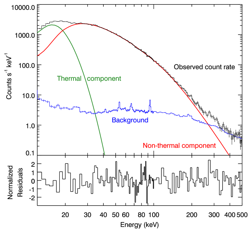
Figure 1.— Example of count spectrum (thick error bars) observed by RHESSI, integrated for 4 seconds around 17-JAN-2005 09:43:36 UT. The spectrum was fitted with a thermal component (Maxwellian), a non-thermal component (log-parabolic, see Appendix A), and the average spectrum before and after the flare, assumed to be the background. For clarity, the total model consisting of the sum of the three components is not plotted over the observed count spectra, but its normalized residuals are shown below instead. The residuals show that the fitted spectral model reproduces the observed counts. The reduced $\chi^{2}$ for this spectrum equals 0.94.

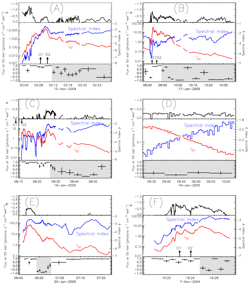
Figure 2.— Temporal evolutions of the spectral index $\gamma$, the flux at 50 keV, $I_{50}$, and the spectral curvature $\eta$ for the selected events. Below, the correlation coefficient between the two curves is shown vs. time. It was determined during the time intervals indicated by the horizontal bars. The vertical bars represent the 68% confidence range. The onset times of the flare associated CMEs are marked by arrows. O1 and O2 indicate linear and quadratic extrapolations, respectively, to the CME altitude vs. time evolution.

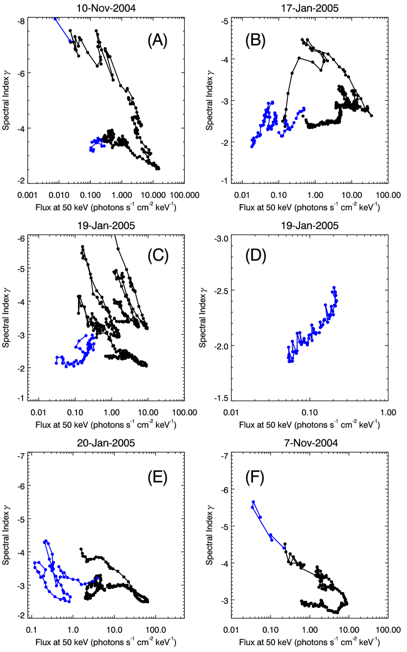
Figure 3.— Evolution of non-thermal X-ray spectral index $\gamma$ vs. photon flux $I_{50}$ in the course of flares.

The goal of this paper is a detailed quantitative study of the spectral evolution of solar flares showing a hardening trend in RHESSI observations. Rather than attempting a statistical study of a large number of flares, the analysis is restricted to a few events studied exhaustively. Therefore, we do not estimate the occurrence frequency of SHH flares or their rate of association with solar energetic particle events. This has been done by Kiplinger (1995) using SMM/HXRBS data, who reports 24 occurrences of hardening out of 152 events with peak flux count rate larger than 5000 counts s^-1. Most of the SHH events reported by Kiplinger are in the upper M and X GOES class. The reality of this trend needs however to be confirmed.

We selected flares with a GOES flux above X1 during RHESSI observation time windows. 50 events satisfying this condition were found in the period from the start of the mission (February 2002) to September 2006. We additionally required that the rise, main and decay phases were well observed to study the spectral evolution in time. This left us with 12 candidates.

As a first approximation, the presence of hardening behavior was tested by studying the count rates in the energy range from 30 to 60 keV. We fitted the spectral index separately in three energy bands (30–40 keV, 40–50 keV, 50–60 keV) and looked for either trends of progressive hardening or the presence of a late hard phase. The lowest of these bands is sometimes contaminated by thermal emission. This can be easily spotted by comparing the time profile with the other bands. Using count rates is adequate to identify candidate events for spectral hardening, but may have missed some events where hardening happens in a phase of low flux close to the background. After discarding two further events with high pileup, we found 5 well-observed events with a clear signature of hardening. These are listed in Table 1.

For each of the selected events, the instrumental response matrices and count-rate spectrograms covering the energy range from 3 to 500 keV were generated for the front segments with a temporal resolution of one RHESSI spin period (approximately 4 s). The spatially integrated photon spectra in the range 12 to 500 keV were fitted with two components: an isothermal component at low energies (below about 20-40 keV) and a non-thermal component at higher energies. The shape of the non-thermal component is assumed to be a log-parabolic curve characterized by three parameters: its normalization $I_{\epsilon_{0}}$ at energy $\epsilon_{0}$, its spectral index $\gamma<0$ and its spectral curvature $\eta$. The functional form of this model (Eq. A1), as well as the rationale for choosing it are explained in detail in App. A. Figure 1 shows an example of an observed count spectrum and the best-fit components. The normalized residuals indicate an excellent fit.

During the fitting process, the model photon spectrum is folded with the response matrix, yielding the expected count spectrum from the model. The background spectrum is then multiplied with a normalization factor $\lambda$ and added to the model counts, where $\lambda$ is an additional fit parameter for the model fitting and is constrained between 0.5 and 2. This correspond approximately to the maximum excursion in RHESSI’s background in the front segments during an orbit. The parameter $\eta$ is constrained to be zero or positive (corresponding to a parabola in log-log bending down). This ensures that the emission approaches 0 for infinitely high energies.

The large amount of data (more than 3 thousand spectra) required an automated fitting routine. For every spectrum, 2 preliminary passes were done estimating the parameters for the thermal and the non-thermal part which were then used as starting parameters for the final fitting. This turned out to deliver good fittings for most of the data. A check of the quality of the fits was performed by looking at the time evolution of $\chi^{2}$ and of the fitting parameters. Spectra with reduced $\chi^{2}$ worse than 2 were manually fitted again, and in most cases it was possible to find another set of fit parameters yielding reduced $\chi^{2}$ below 2, with the exception of the event of 20-JAN-2005.

This event (the largest flare, GOES class X7) is characterized by very strong thermal emission. At times when the non-thermal emission is weak and/or soft, pileup effects are especially large in the 20-50 keV band. Therefore, the fittings, which are good above 50 keV, have large residuals below that energy. This may be due to the fact that the photon spectrum model chosen is not suited to describe the observed photon spectra, or that the pileup correction is inaccurate. Because it is very hard to correctly take into account pileup effects in such a regime, it is not clear whether the model failure is real or instrumental. Therefore, we let the spectrum model stand as it is, but caution that the parameter values fitted in the flare of 20-JAN-2005 may be less accurate, due to the unknown systematic effects generated by imperfect pileup correction.

For the other events, the fit parameters are of good quality and the corresponding photon models are a high-fidelity representation of the incoming photon flux. The final distribution of the reduced $\chi^{2}$ for all events (except 20-JAN-2007) is such that 89% of all spectra have $\chi^{2}$ less than 1.5 and 97% of all spectra have $\chi^{2}$ less than 2. Therefore the unusual choice of the logarithmic parabolic fit-model, explained in Sect. 2, produces good fittings and is therefore justified a posteriori.

Three of the events presented here have also been studied by Saldanha et al. (2008), where the non-thermal component has been fitted by a double power-law. The temporal evolution of our values for $\gamma$ (at 50 keV) is very similar to theirs, although the actual numerical values are slightly different due to the different fitting methods employed and their choice of energy intervals. The differences are larger for the January 20 event, where they used the 100-200 keV energy interval.

The thermal evolution of the events shows a rapid increase of the emission measure at the beginning of the event, followed by a flat peak and a slow decay. The temperature is in the range 20-40 MK, peaks before the emission measure and decays faster.

3. Spectroscopy Results

Figure 2 shows time profiles of the photon spectral index $\gamma$ and the flux normalization at 50 keV, $I_{50}$ (given in Eq. A1), for the events of Table 1, as found by the spectral fitting procedure explained in Sect. 2 and Appendix A.

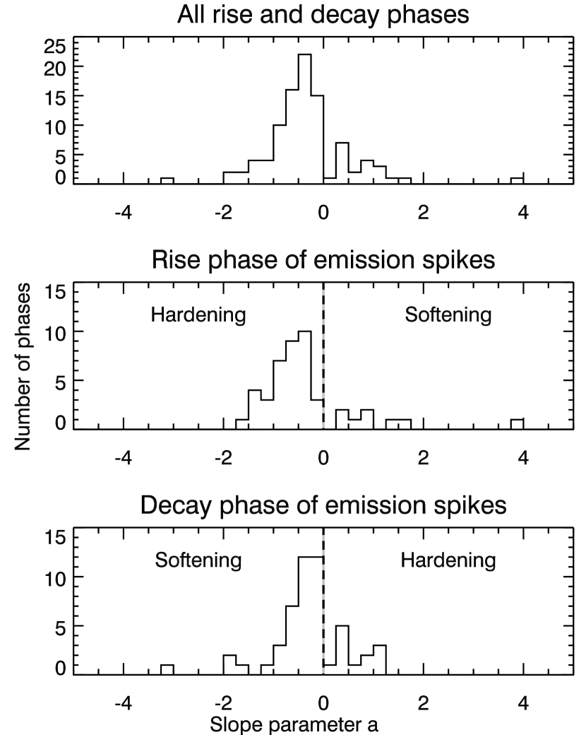
Figure 4.— Distribution of the slope in $\gamma$ vs. log($I_{50}$) (Fig. 3, parameter $a$ in Eqs. 1 and B1) for the rise and decay phases in all peaks of the observed events (upper panel) and for rise and decay phases separately (middle and bottom panel, respectively).

The observed spectral variability of flares on time scales down to ten seconds or less requires the highest possible temporal resolution for the spectral fitting (about 4 seconds in our case). Longer integration times, while desirable for better photon statistics, are not suitable because the averaging effect of summing spectra with different hardness blurs the spectral evolution. Nevertheless, during the decay phase the flux is so low that full resolution spectra deliver noisy values for the fitting parameters. In this case, longer integration times must be used. This is acceptable, since the variations of the hard X-ray flux are slower during the decay phase, and short-lived spikes are less frequent. Therefore, some light curves shown in Fig. 2 and subsequent figures use a lower cadence of approximately 32 seconds (that is, 8 RHESSI rotations) in the decay phase.

Short gaps lasting about 1 minute can be seen in the light curves (Fig. 2). They correspond to periods where the thick attenuator was removed from the field of view, but the X-ray flux was still so large that the dead time in the detector prevents meaningful spectral analysis.

The selected flares show many distinct SHS peaks. They are characterized by a temporal correlation of $\gamma$ and $\log I_{50}$, yielding roughly parallel curves in Fig. 2. On the other hand, in the presence of SHH peaks or progressive hardenings, the two time profiles diverge. This may be illustrated in the event of 19-JAN-2005 (Fig. 2, panel C), where the two profiles run roughly parallel until 08:29 and then start to diverge.

To better distinguish between the SHS and the hardening trends, Fig. 2 also shows the correlation coefficients between the spectral index $\gamma$ and the logarithm of the flux $\log I_{50}$ vs. time. The vertical bars represent the 68% confidence range (corresponding to one standard deviation). SHS peaks are characterized by a correlation coefficient close to +1. Times, on the other hand, when the spectrum hardens while the flux becomes lower have a negative value of the correlation coefficient. We note that during the SHS times correlation is rather constant (near +1), whereas during the hardening phase the correlation coefficients are more erratic and often not close to -1. This indicates that it may not be possible to find a behavior similarly well-defined for the periods of hardening as it is found for the SHS peaks. In some cases (19-JAN-2005, 08:28 to 08:30), the spectral hardness stays nearly constant while the flux decays. This yields a correlation coefficient near zero.

It should be noted here that most periods showing hardening have low flux. Therefore the corresponding time profiles may be more noisy, weakening the correlation. Some of this effect was compensated by increasing the time interval for correlation. Another effect is loss of correlation during a broad peak. Again this can be taken into account by increasing the correlation interval.

During the late phase of the event of 19-JAN-2005, in the RHESSI orbit following the one featuring the main peak, an uninterrupted phase of hardening is seen. From 09:35 to 10:00 the flux decays exponentially (see Fig. 2, panel D). After that time, the emission reaches a hardness comparable with the one of the background, and it becomes impossible to disentangle the two components by purely spectral methods. This event will be investigated in more detail in Section 5.

We also compared the start of the hardening with the onset time of flare-associated CMEs, taken from the SOHO LASCO CME catalog (Yashiro et al., 2004). In three cases (panel A, B, and F in Fig. 2), the onset of the CME precedes the start of the hardening by 3 to 5 minutes, in one case by 15–20 minutes (panel C) and in one case by 50 minutes (panel E). In all five events an associated CME was present, but the hardening phase never starts before the CME onset.

Figure 3 shows the relationship between $\gamma$ and $\log I_{50}$. Since the flux increases from left to right and the hardness increases from top to bottom, SHS peaks show as piecewise linear trends with a negative slope (Grigis & Benz, 2004, 2005a). On the other hand, progressive hardening during flux decay is visible as a trend with positive slope. Such relations can be written as

$$\gamma=-a\log(I_{\epsilon_{0}})+b\,,$$ (1)

where $a<0$ for the SHS peaks and $a>0$ during hardening phases. The minus sign in front of $a$ takes care of the fact that in Fig. 3 the vertical axis for $\gamma$ is reversed.

Careful examination of the plots in Fig. 2 and 3 reveals that

• Most of the emission spikes are well represented by straight lines in $\gamma$-$\log I_{50}$ during the rise and decay phase. The decay phases are sometimes flatter in $\gamma$-$\log I_{50}$ than the corresponding rise phases (e.g. panel C), but the opposite is also observed (panel A). The event shown in panel E shows some significant deviations from the piecewise straight trend.

• Spectral variability is stronger at the beginning of the event (panels A, B, C, F).

• In the late phase of the events a slower varying component is seen, piecewise straight in $\gamma$-$\log I_{50}$, mostly nearly flat, slowly hardening (panels B, D), slowly softening (panels A, F), staying at an approximate constant hardness (panel C), or a mixture of the above (panel E).

• During the rise phase up to the strongest peak, the hardness tends to increase from peak to peak (panels A, C). Events are softer in the beginning (all panels).

Figure 4 shows the distribution of the $\gamma$-$\log I_{50}$ slopes (parameter $a$ in Eqs. 1 and B1) in the rise and decay phases of all emission spikes in the 5 events. If the flux increases, a negative slope represents spectral hardening and a positive slope a softening. The opposite happens during a decay phase. SHS peaks have $a<0$ both in the rise and decay phase.

The separate histograms for rise and decay phase differ marginally. Spectral hardenings during rise have a slightly steeper $\gamma$-$\log I_{50}$ slope than softenings during decays (SHS peaks). Quantitatively, the average value of $a$ when restricted to negative values is of $-0.70\pm 0.06$ (the uncertainty is the standard error of the mean) during the rise phases and $-0.51\pm 0.08$ during the decay phases (after removing an outlier with slope -3.2). The average of $a$ for the combined set of rise and decays is $-0.60\pm 0.05$, corresponding to an average pivot point energy (see App. B) of $\epsilon_{*}=9.4\pm 1.3$ in agreement with Grigis & Benz (2004).

Examination of spectral hardenings during decay and softenings during rise phases (trends opposite to SHS), restricted to the range 0–3, yield an average $a$ value of 0.66$\pm$0.11 and 0.88$\pm$0.18, respectively. These values are not significantly different from each other or from the corresponding absolute value of the $a<0$ averages.

4. Imaging results

Table 2Source motion near the onset of hardening.

Event	Onset of	Footpoints	Coronal source
	hardening	motion	motion
07-NOV-2004	16:26	Jump in the position of the eastern FP	uncertain (bad images at
		Change in the direction of motion of the western FP	low energies after onset)
10-NOV-2004	02:12	Jump in the position of the two brighter FPs	stationary
17-JAN-2005	09:49	Nearly continuous motion of both FPs	continuous motion
19-JAN-2005	08:27	Continuous motion of the northern FP, slowing after the onset	continuous motion upward
		Nearly stationary position of the southern FP
20-JAN-2005	06:49	Reversal in the direction of motion of both FPs, slowing down afterwards	continuous motion upward

Is there a connection between spectral hardening and X-ray source geometry indicating a different acceleration site? The position of the hard X-ray footpoint sources were investigated in CLEAN images, using detectors 3 to 8 with a cadence of 60 seconds. In particular, we looked for differences in source positions and velocities at the onset and during the period of general hardening.

Figure 5 shows an overview of the position of the thermal and non-thermal sources during the events. The event of 10-NOV-2004 is not shown because it lacks a coordinated evolution of source positions.

The event of 19-JAN-2005 is particularly interesting, as it was well observed and the footpoints (FP) clearly move along the ribbons noticeable in a TRACE image at 1600 Å (Saldanha et al., 2008). The motion is fast at the beginning and later slows down. The thermal source has the form of a loop, rising throughout the event.

Figure 6 shows the displacement of the northern FP source in the directions parallel and perpendicular to the northern ribbon. The FP source starts with a velocity of 50 km s^-1 along the ribbon and slows down continuously during the SHS phase until the onset of the hardening phase, when it becomes nearly stationary. There is no evidence of an abrupt transition between the two regimes. Furthermore, 19-JAN-2005 is the only event clearly showing footpoints drifting apart and coming to a stop at the onset of hardening.

The other events show other positional changes. In the following the geometrical behavior of the sources and their evolution are described shortly for all the events. We distinguish between footpoint sources and coronal sources. Because of projection effects, we cannot reliably reconstruct the three dimensional structure of the sources. However we know from limb event observations (Battaglia & Benz, 2006) that FP sources are mainly non-thermal and well-observed above 20-30 keV, whereas coronal sources are mainly thermal and well-observed below 20-30 keV. Therefore, we assume in the following that the thermal source is coronal and that non-thermal sources are footpoints.

07-NOV-2004: This events features two footpoints and a coronal source. The eastern FP moves from W to E from 16:20 to 16:24 UT, jumps back to near the starting position and moves again from W to E from 16:25 to 16:30. The western FP moves slightly from SW to NE from 16:21 to 16:24, then changes direction with a slight jump to W, and slowly moves to NW from 16:25 to 16:30. The western FP is brighter than the eastern FP before 16:24 and dimmer after 16:25. The thermal source is located farther E than the FPs and moves slightly to N from 16:19 to 16:25, and is not clearly seen in the images afterwards, due to the insertion of RHESSI’s thick attenuators.

The jump in position around 16:25 roughly coincides with the time at which the hardening starts, possibly indicating that another loop is actively accelerating electrons, but the expansion of the loop, as suggested by the FP motions, continues during the hardening phase, contrarily to what has been observed in the event of 19-JAN-2005.

10-NOV-2004: This event has a very complicated FP morphology, with sources and source-pairs appearing in many different places. It is not possible to find a well-defined source motion like in the simpler cases with only two footpoints. Here the sources seem to jump around as new footpoints in a different position become brighter and outshine the old ones. Important shifts in position occur at 02:08 and 02:12. The latter shift happens at the same time as the onset of hardening.

17-JAN-2005: Three pairs of FPs are seen. The northern pair is stationary and seen from 09:43 to 09:45. The southern pair consists of an eastern FP moving to SE from 09:45 to 10:05, and a western FP moving to N from 09:43 to 09:47, then shifting to W (09:55) and moving very slowly to N until 10:05. The last pair of FP is to the east and stationary from 10:11 to 10:29. Coronal sources are seen in two locations: one to the N of the southern FP pair, moving to N from 09:46 to 09:57, and the second to the NW of the easternmost FP pair, nearly stationary from 10:16 to 10:30.

There is no clear signature of a discontinuity or a change of behavior happening around 09:50, when the hardening starts.

19-JAN-2005: Two footpoints are seen with a loop-shaped coronal source between them. The northern FP moves to NE from 08:12 to 08:30 (covering nearly 60 arcseconds) while the southern FP moves, slower, to SE. In the meantime, the loop-shaped coronal source moves to NW (indicating that it is rising). After 08:30 (only 3 minutes after the onset of hardening) the northern FP is much slower. The coronal source keeps moving to NNW. In the next RHESSI orbit (after 09:30), the FP sources can still be seen near the old positions at 08:30. The northern FP is nearly stationary from 09:33 to 09:59, while the southern FP very slightly moves to W, and the coronal source slightly moves to N.

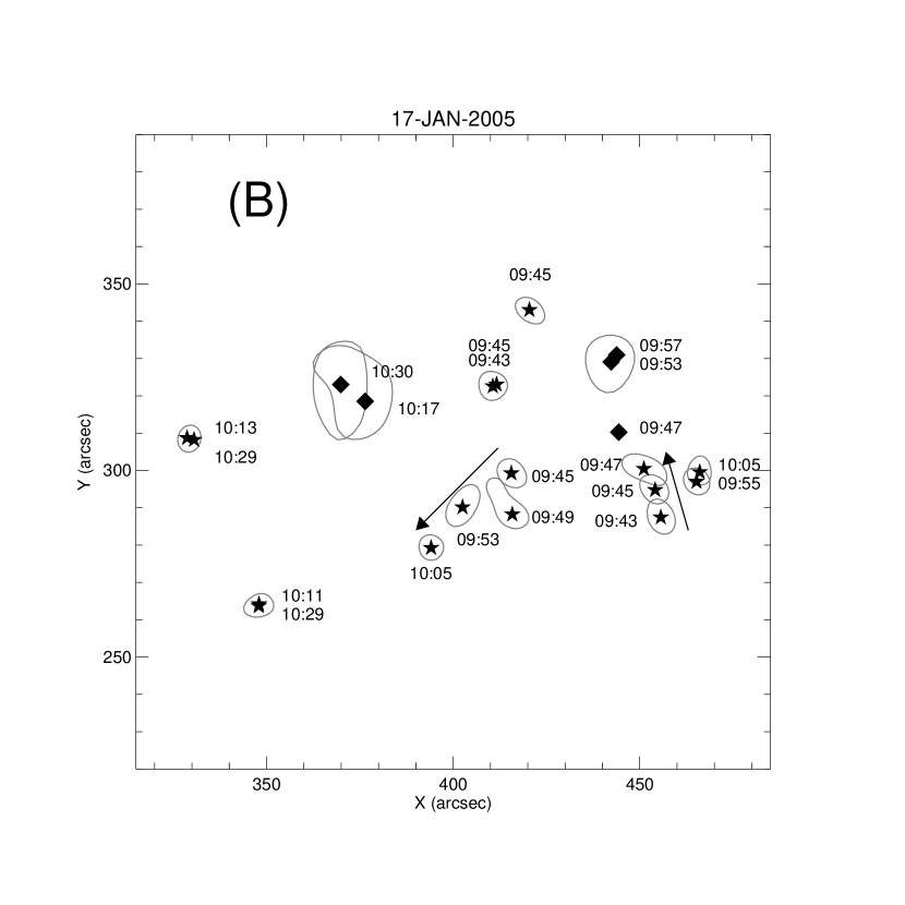
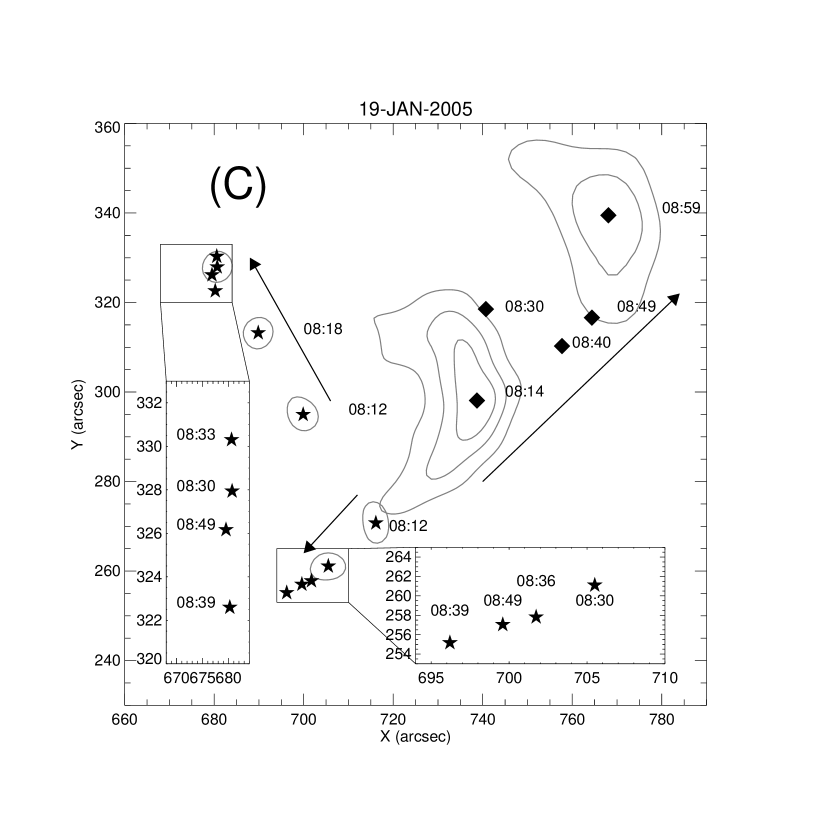
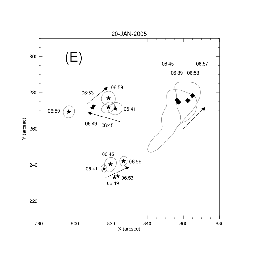
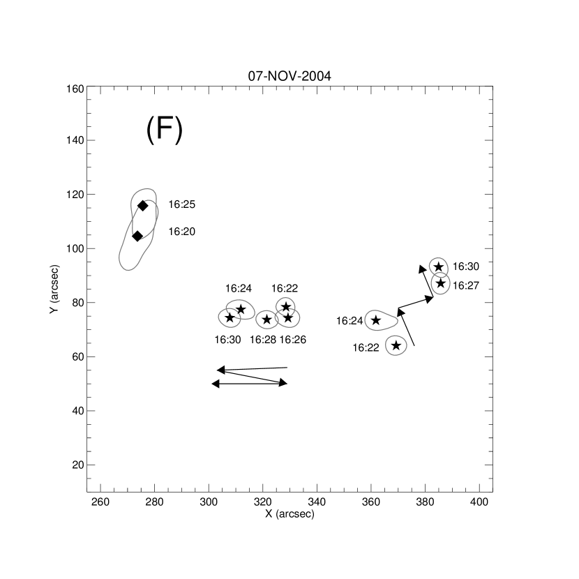
Figure 5.— RHESSI hard X-ray positions of the non-thermal footpoint sources (stars) and the thermal coronal source (diamond) for 4 events. The energy range for the footpoint position is 50-100 keV band (or 25-50 keV at times where the 50-100 keV emission is too faint for imaging). The energy range for the coronal source position is 12-25 keV. Systematic motions are indicated by arrows.

20-JAN-2005: This near-limb event features two FPs and a loop-like coronal source. The southern FP moves to W while the northern FP moves to E. The eastward motion of the northern FP is not continuous: at 06:49 it reverses and recedes until 06:55, when another sources appears 20^′′ to E. The double structure lasts until 07:01, when the easternmost source fades away. The coronal source moves to NW and rises throughout the event, slowing down towards the end. The reversal coincides with the start of the hardening phase.

The observed behavior at the onset of hardening for all events is reported in Table 2. It summarizes the analysis of the source motions in an interval of time spanning 4 minutes, centered on the onset of hardening. We conclude from the imaging observations that there is no universal trend holding for all events. Sometimes, there seems to be a switch to a different loop system near the beginning of the hardening phase. On the other hand, such jumps can also be seen during the SHS phase of the events, so they need not be significant. There is also some indication that the FP motion is slower during the hardening phase, but again this does not hold for all events. In the event of 19-JAN-2005, with a simple geometry and well observed, the change in spectral behavior leading to the hardening phase does not have an impact on the morphology of the hard X-ray sources seen by RHESSI.

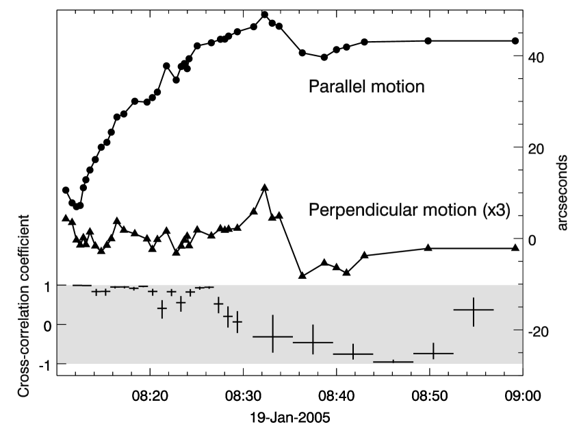
Figure 6.— Movement of the northern X-ray footpoint source for the event of 19-JAN-2006. The upper curves show the motion in the two components parallel (top curve) and perpendicular (middle curve, multiplied by a factor of 3) to the northern TRACE 1600 Å ribbon. The bottom curve displays the cross correlation coefficient between hard X-ray spectral index and flux, showing the onset of spectral hardening around 08:27.

5. Modeling the SHH phase

Grigis & Benz (2006) showed that the soft-hard-soft trend is expected from a transit-time damping stochastic acceleration model that includes escape of particles from the accelerator. The hardness is controlled by how fast the particle gain energy and how long they are trapped in the accelerator. Harder spectra result from longer dwelling times of the electrons in the accelerator and higher acceleration efficiency. These conditions also allow a larger population of high-energy electrons to build up, leading to increased hard X-ray emission from the accelerator, identified as a part of the looptop source. This basic model predicts that harder spectra also have larger hard X-ray flux, but cannot explain the soft-hard-harder trend seen as the flux decays, because these observations associate harder spectra with smaller flux.

To fit the observed SHS behavior, Grigis & Benz (2006) had to assume that electrons are trapped below a certain threshold energy $E_{\mathrm{T}}$ and cannot leave the accelerator. The escaping electron population has a low-energy cutoff at $E_{\mathrm{T}}$. Then the photon spectra of the footpoints, which dominate the non-thermal emission, harden below $E_{\mathrm{T}}$.

In the following, a simple extension of the basic stochastic acceleration model is presented which could lead to the observed spectral hardening. We introduce the additional assumption that $E_{\mathrm{T}}$ increases with time in the SHH phase. Therefore, the photon spectrum below $E_{\mathrm{T}}$ hardens while at the same time the flux arriving at the footpoints decreases. The important point here is that this also happens if the electron spectral index $\delta$ and the electron flux normalization in the acceleration region are constant. Thus the new variable does not contradict the basic properties of the stochastic acceleration model. This is shown in Fig. 7, where footpoint photon spectra have been computed from a given electron distribution with various $E_{\mathrm{T}}$. As expected, the photon flux decreases with increasing $E_{\mathrm{T}}$. Note that the photon spectra have a nearly constant but slightly increasing hardness while the flux decreases.

This extension is compared numerically to the late phase of the 19-JAN-2005 event. For simplicity, an electron distribution with constant spectral index and flux normalization is assumed to escape from the acceleration region. It has a low-energy cutoff $E_{\mathrm{T}}$ due to trapping in the accelerator. $E_{\mathrm{T}}$ increases with time. Obviously, we do not expect such a simple scenario to reproduce all the details of the spectral evolution. The question is, how much of the observed features can be explained with this simplest extension of the existing acceleration model.

A non-isotropic energy distribution of fast electrons with a positive slope in energy is known to be unstable towards growing plasma waves. Therefore our scenario also includes an alternative electron distribution featuring a turnover at $E_{T}$, that is, a flat distribution below $E_{T}$, instead of a cutoff. The electron distributions with cutoff and turnover are assumed as,

$$F_{\mathrm{CUTOFF}}(E) = \left\{\begin{array}[]{lll}F_{E_{0}}\left(\displaystyle\frac{E}{E_{0}}\right)^{\delta}&\mathrm{if}&E\geq E_{\mathrm{T}}\\ 0&\mathrm{if}&E<E_{\mathrm{T}}\\ \end{array}\right.$$ (4)

$$F_{\mathrm{TURNOVER}}(E) = \left\{\begin{array}[]{lll}F_{E_{0}}\left(\displaystyle\frac{E}{E_{0}}\right)^{\delta}&\mathrm{if}&E\geq E_{\mathrm{T}}\\ F_{E_{0}}\left(\displaystyle\frac{E_{T}}{E_{0}}\right)^{\delta}&\mathrm{if}&E<E_{\mathrm{T}}\end{array}\right.$$ (7)

The free parameters are the electron spectral index $\delta$, the electron flux normalization $F_{E_{0}}$ (electrons s^-1 keV^-1), the cutoff or turnover energy $E_{\mathrm{T}}$. The reference energy $E_{0}$ is fixed at 50 keV.

An exhaustive description of the method used for the comparison of this simple model with the observation and finding the best fit is given in App. C.

The late phase of the event of 19-JAN-2005, from 09:32 to 10:02, comprises 30 minutes of continuous hardening, and therefore is well suited for the comparison with the variable cutoff model. Figure 8 shows the comparison. The observed values of $\gamma$ and $\eta$ are plotted as a function of $I_{50}$ together with the best-fit model curve for both the cutoff and turnover electron spectra. For the cutoff model, the best fit values of the parameters are: spectral index $\delta=6.52$, flux normalization at 50 keV $F_{50}=4.50\cdot 10^{33}$ electrons s^-1 keV^-1. In the course of the decay, $E_{\mathrm{T}}$ increases from 98 keV to 159 keV (thus yielding a photon spectral index $\gamma$ in the range between -2.5 and -1.9). The corresponding values for the turnover model are: $\delta=6.11$, $F_{50}=3.67\cdot 10^{33}$ electrons s^-1 keV^-1, while $E_{\mathrm{T}}$ increases from 127 to 224 keV.

The photon spectra from both the cutoff and turnover model are curved downward in the fitted energy range. Thus the spectral curvature, $\eta$, is negative. It is observed to be between 0 and -0.3, whereas the model spectra have values in the range from -0.55 to -0.25 (Fig. 8, bottom) and thus are significantly more curved.

In the cutoff distribution, the total fluxes of electrons escaping the acceleration site are initially $9.9\cdot 10^{32}$ electrons s^-1 above $E_{\mathrm{T}}=98$ keV. This reduces to $6.6\cdot 10^{31}$ electrons s^-1 for $E_{\mathrm{T}}=159$ keV in the course of the decay. The total injected power reduces from $1.9\cdot 10^{26}$ erg s^-1 to $2.1\cdot 10^{25}$ erg s^-1. In the turnover model, the total number of particles diminishes from $2.3\cdot 10^{33}$ to $1.3\cdot 10^{32}$, and the injected power from $1.9\cdot 10^{26}$ erg to $2.8\cdot 10^{25}$ erg.

6. Discussion

Spectroscopic RHESSI observations are well suited to study the spectral evolution during the main phase of large flares. The path observed in the $\gamma$ vs. $\log I_{50}$ plots for the events is not simple. However, it can be broken down reasonably into a superposition of linear sections during flux rise and decay phases. While not all rise or decay phases can be so decomposed, this simple description is adequate for most of them, and permits comparison of observations and theory.

There is a difference between the results reported here and the results from Grigis & Benz (2004) in the asymmetry between rise and decay phases in SHS peaks. The previous results indicated that decay phases are steeper in the $\gamma$ vs. $\log I_{50}$ plot than rise phases. We find the opposite. The reason is probably the selection bias: here we selected specifically events showing hardening. This hardening trend sometimes overlays SHS peaks, giving rise to a soft-hard-less-soft pattern.

The hard X-ray images during the events show the usual morphology of hard X-ray solar flares: a low-energy coronal source and two or more high-energy footpoint sources. The position of the footpoint sources is strongly variable: it either moves smoothly or jumps from location to location. This reflects changes in the connection between the accelerator and the chromosphere, as well as in the location of the accelerator itself.

The behavior observed in the images cannot be reduced to one simple scenario valid for all events. However, the observations suggest that there is no clear separation between the SHS and the hardening phases: the former seems to smoothly merge into the latter. Even in the cases where the emission jumps at the onset of hardening (Table 2), the footpoint behavior seems not to change radically.

Figure 7.— Photon spectra by thick target emission (at footpoints) from a constant power-law electron distribution having spectral index of $\delta=-6.5$ in the acceleration region. The low-energy cutoff, $E_{\mathrm{T}}$, increases from the top to the bottom curve from 0, 100, 120, 140, to 160 keV.

Alternatives to the scenario presented in Sect. 5 are conceivable. In particular, electron storage in the corona and slow release during the decay could be a possibility. As Coulomb interactions are faster at low particle energies, the spectrum would harden with time while the released flux decreases. Noting that the hardening phase in the 19-JAN-2005 event lasts more than 30 minutes and that the decay of the flux in time is nearly exponential (as seen by the fact that the $I_{50}$ line in Fig. 2, panel D, is nearly straight), the total number of injected electrons can be computed from the total electron fluxes at the start $F_{\mathrm{BEG}}$ and at the end $F_{\mathrm{END}}$.

$$F_{\mathrm{TOT}}=\Delta t\frac{F_{\mathrm{END}}-F_{\mathrm{BEG}}}{\log\displaystyle\frac{F_{\mathrm{END}}}{F_{\mathrm{BEG}}}}\,,$$ (8)

where $\Delta t$ is the observed duration (here 30 minutes) and $F_{\mathrm{TOT}}$ the total injected flux. From the observed values, we get $F_{\mathrm{TOT}}\simeq 1\cdot 10^{36}$ electrons for the turnover model and $F_{\mathrm{TOT}}\simeq 6\cdot 10^{35}$ electrons for the cutoff model. These numbers do not seem extraordinarily high, but it should be noted that all these electron have energies above 100 keV.

Would such a large population of electrons be seen as a coronal hard X-ray source in the 50 - 100 keV band? The luminosity depends on the volume and density in the storage region. The observed footpoints in the hardening phase are separated from each other by approximately 60^′′, indicating a medium sized loop. Therefore, it would be visible on RHESSI images unless it were excessively under-dense. Thus we reject the storage model.

Both the cutoff and turnover model are able to reproduce the observed $\gamma$ vs. $\log I_{50}$ trend, but fail to reproduce the correct spectral curvature $\eta$ (Fig. 8). Although the observation of $\eta$ is more difficult in the decay phase due to the lower signal-to-background ratio, the difference between the cutoff and turnover models and the observed points is significant. The value of the parameter $\eta$ depends on the energy interval chosen for the fitting of the model photon spectra (20-80 keV in our case). A lower maximum energy of this interval produces lower model values for $\eta$.

We note furthermore that if the accelerator is inhomogeneous, the electron spectrum at the footpoints is the superposition of different components with different values of the low-energy cutoff or turnover $E_{\mathrm{T}}$. The superposition of spectra that curve at different energies is less curved than individual spectra. Figure 7 suggests that the superposition of components with different spectral shape may in fact reduce of the total spectral curvature. Thus we consider the disagreement in curvature not crucial to reject the model.

7. Conclusions

We have presented results of spectroscopy, imaging and simple modeling of spectral hardening observed occasionally in the hard X-ray emission of large flares. The main conclusions are:

• The flares selected for the presence of a hardening phase also show soft-hard-soft behavior, at least initially. The hardening starts at or after the largest peak of the flares. In 3 out of 5 events it starts 2 to 6 minutes after the onset of a CME.

• Similar to SHS peaks, hardening phases can usually be described by piecewise linear sections in a plot of spectral index vs. logarithmic flux.

• There is no clear trend relating the behavior of hard X-ray footpoint sources with the spectral evolution that would be valid for all events. Sometimes the location of the emission shifts when the hardening starts, in other events it does not.

• In the event of 19-JAN-2005, there are only two well-defined footpoint sources throughout the whole event. No discontinuity is observed in the motion at the onset of hardening, but a general trend of slowing down, such that the FPs become nearly stationary during the decay phase.

• In 3 out of 5 flares, the coronal source moved continuously during the onset of the hardening. This motion was directed upwards in two near-limb events.

Figure 8.— Observed values of $\gamma$ vs. $I_{50}$ (top panel) and $\eta$ vs. $I_{50}$ (bottom panel), represented by asterisks. The best-fit model curves (continuous for the cutoff model, dashed for the turnover model) are expected from model with constant electron hardness and flux, but rising low energy cutoff or turnover energy $E_{\mathrm{T}}$.

In the sample studied, we find a surprising lack of detailed correlation between spectral and spatial behavior. It is similar to what has been observed by Grigis & Benz (2005b) in a smaller flare (M6) featuring strong footpoint motions and hardening at the end.

The main question addressed in this paper is whether the SHS peaks and the hardening phases are the results of two different acceleration mechanisms. The results support the view that the same acceleration mechanism changes gradually in the later phase of the flare. This change has clear effects on the spectrum, but a more indirect and subtle influence on the source position. The operation of a second acceleration process later in the flare cannot be ruled out, however. Nevertheless, we have found strong evidence that there is a gradual change in the accelerator, transforming its behavior from impulsive (showing up as SHS peaks) to gradual (hardening phases). This is substantiated by the observations of the superimposition of SHS peaks with a continuous hardening trend and of the smooth footpoint motions during the onset of hardening.

The reason for the association with interplanetary proton events (Kiplinger, 1995) remains to be explored. As an aside we may note that when the footpoints drift apart, acceleration takes place in larger and larger loops. In a stochastic acceleration framework, the acceleration efficiency of electrons in larger loops is reduced, while ions can be more efficiently accelerated (Emslie et al., 2004). Since hardening trends are well correlated with the occurrence of interplanetary energetic protons events, it is possible that the very conditions that are responsible for the hardening trends favor acceleration of protons, which may then escape into interplanetary space, with the CME controlling their release rather than acceleration (Simnett, 2006).

The observed motion of footpoints suggests that different coronal loops may be involved in particle acceleration during a flare. They will have different physical properties such as size, density, and magnetic field. The overall magnetic geometry of the active region will determine which loops reconnect at which time, sometimes giving rise to an orderly motion of footpoints, sometimes generating a more chaotic situation. The data suggest that as the reconnection process proceeds, some physical parameters of the acceleration site changes in such a way as to favor the production of harder spectra, rather than having a totally new process (say, shock acceleration) taking over in the decay phase.

Appendix A Hard X-ray model fitting

The hard X-ray spectrum observed in solar flares consists of two distinct components at low energies (that is, below 10-40 keV) and high energies. The properties of the low-energy component are typical of thermal emission of a hot plasma with temperature of 10 to 40 MK. In particular, the spectrum steepens with energy, and the temporal evolution follows the (cooler) thermal plasma observed in soft X-rays and EUV.

The high-energy component behaves differently and is hence dubbed non-thermal. It is harder then the thermal component and is usually fitted with a power-law function of the energy with 2 free parameters. However, sometimes the observed spectrum steepens at higher energies. In the literature, this is usually accounted for by using a broken power-law model (e.g. Dulk et al., 1992; Battaglia et al., 2005). There are some disadvantages in the broken power-law model: a) it is not physical, in the sense that any continuous electron distribution emitting X-rays should generate a differentiable photon spectrum, and b) the location of the break-point is poorly determined by the observations.

We argue that there is a simpler extension to the power-law model which both turns down at higher energies and is smooth. Recalling that a power-law function plotted in log-log space is a straight line, we choose as a “natural” extension to the next order a parabolic model in log-log space, described by the function

$$I(\epsilon)=I_{\epsilon_{0}}\cdot\left(\frac{\epsilon}{\epsilon_{0}}\right)^{\displaystyle\gamma-\eta\log\left(\epsilon/\epsilon_{0}\right)}\,.$$ (A1)

The 3 model parameters are the normalization $I_{\epsilon_{0}}$, amounting to the flux at the (fixed) normalization energy $\epsilon_{0}$, the spectral index $\gamma<0$ and the parabolic coefficient $\eta$, which we will refer to as the spectral curvature although, strictly speaking, the geometric curvature of the parabola is not constant, but equals $-2\eta$ in the vertex and vanishes at infinity.

In the special case $\eta=0$, the (unbroken) power-law model is recovered. We note here that a log-parabolic model has been used previously to describe observed X-ray spectra of pulsars (Massaro et al., 2000).

In summary, the reasons for preferring the log-parabolic model over the more usual broken power-law are:

1. It is simpler than the broken power-law, as it allows only 3 instead of 4 free parameters.

2. For the vast majority of the time intervals, it produces similar values of $\chi^{2}$ as the broken-power law.

3. It is differentiable, therefore there exists a continuous electron spectrum producing the photon spectrum. This is not the case for the broken power-law, where a discontinuity is needed in the electron spectrum, which would quickly be eliminated by kinetic plasma processes. The spectral index increases linearly with $\log\epsilon$.

4. It allows a better comparison with acceleration models which naturally produce slightly curved electron spectra (like stochastic acceleration).

Therefore, we fit the spectra to a photon model with an isothermal component at lower energies and a log-parabolic component as given above at higher energies. The background is taken into account in the following way: the pre-event and post-event background spectra are measured and averaged (in some cases, particle contamination prevented to obtain both of them, and only one was taken instead), yielding a reference background spectrum. The reference background spectrum is multiplied with a free parameter $\lambda$ and added to the model spectrum. $\lambda$ is fitted together with the other model parameters.

In large flares, sometimes an additional hard and weak $\gamma$-ray emission from electrons is observed above 200 keV (Krucker et al., 2008). In this paper we do not report on the properties of this emission since it is not related to the hardening of the spectrum at lower energies. Does this component negatively affects our fittings? Examination of the fitted spectra reveal that the fittings account for this weak, hard emission by an increase of the parameter describing the strength of the background ($\lambda$) by a factor of about 1 to 2. The fittings are of good quality because the background is also weak and hard. This erroneous increase in the strength of the background has no effect at lower energies, since there the hard X-ray flux is stronger by orders of magnitude.

Appendix B Pivot point and parabolic fitting

A linear dependence of $\gamma$ vs. $\log I_{\epsilon_{0}}$ with negative slope can be interpreted geometrically as a fixed intersection point of the various power-law spectra at different times. The intersection in the spectral plane ($I$ vs. $\epsilon$) is called the pivot point, located below the reference energy $\epsilon_{0}$ (Grigis & Benz, 2005a). Similarly, a linear dependence with positive slope can be interpreted by a pivot point at energy larger than $\epsilon_{0}$. If fitting a log-parabolic spectrum, it is the tangents to the spectrum at $\epsilon_{0}$ in log-log space that are intersecting, rather than the curves themselves.

The description in terms of a pivot point has the advantage that it does not depend on the choice of the reference energy $\epsilon_{0}$. On the other hand, the pivot point energy jumps from $0$ to $+\infty$ when the slope in $\gamma$-$\log I_{\epsilon_{0}}$ goes from negative to positive. The relation between the pivot point coordinates $\epsilon_{*},I_{*}$ and the line parameters $a,b$ in Eq. 1 are given by

$$\qquad a=\frac{1}{\log\left(\epsilon_{*}/\epsilon_{0}\right)}\qquad\qquad b=\frac{-\log{I_{*}}}{\log\left(\epsilon_{*}/\epsilon_{0}\right)}\,.$$ (B1)

Since the spectra are curved in log-log space, the local spectral index $\gamma^{\prime}$, defined as the logarithmic derivative of the spectrum

$$\gamma^{\prime}(\epsilon)=\frac{\partial\log I(\epsilon)}{\partial\log\epsilon}=\gamma-2\eta\log(\epsilon/\epsilon_{0})\,,$$ (B2)

is energy dependent. The spectral parameter $\gamma$ is equal to the local spectral index $\gamma^{\prime}$ at the reference energy $\epsilon_{0}=50$ keV. The presence of a strong correlation of the time series of $\gamma$ and $\log I_{50}$ does not necessarily imply a strong correlation of the time series of $\gamma^{\prime}(\epsilon)$ and $\log I(\epsilon)$ at energies $\epsilon\neq\epsilon_{0}$. In fact, if the spectra have a common pivot point at $\epsilon_{*}<\epsilon_{0}$, the correlation of $\gamma^{\prime}(\epsilon)$ and $\log I(\epsilon)$ weakens near the pivot point, and turns into an anticorrelation for $\epsilon<\epsilon_{*}$. On the other hand, if a pivot point exist at $\epsilon_{*}>\epsilon_{0}$, then the anticorrelation between $\gamma^{\prime}(\epsilon)$ and $\log I(\epsilon)$ for $\epsilon\simeq\epsilon_{0}<\epsilon_{*}$ transforms itself into a correlation at $\epsilon>\epsilon_{*}$.

An examination of the data for the events studied here shows that in the time intervals when the correlation coefficient between $\log I_{50}$ and $\gamma$ is near 1, the correlation coefficient between $\gamma^{\prime}(\epsilon)$ and $\log I(\epsilon)$ is approximately constant at energies higher than 30-40 keV However, it shows a strong decrease to values close to -1 at lower energies such that the transition takes place around 5-20 keV, near the pivot point position. On the other hand, when the correlation coefficient is near -1 at 50 keV we observe that the correlation coefficients rises toward 1 at higher energies, as these events tend to have a pivot point at energies larger than 50 keV.

Therefore, the energy dependence of the correlation in the data follows a similar pattern as the one expected for non-curved spectra. This is because the observed spectra are not strongly curved: $\eta<0.25\gamma$ in all the fitted spectra, and $\eta<0.15\gamma$ in 85% of all fitted spectra.

Appendix C Comparison between model and observation

Comparison of non-thermal hard X-ray spectral observations and theoretical models can be performed in different ways. In our case, we have a really simple model and a time-dependent situation. The goal of the comparison is not the perfect reproduction of every single observed spectrum, but rather a coherent description of the time evolution which should be compatible with the observed data. This is implemented by the additional constraint in the model (as given by Eq. 4) of keeping a constant electron spectral index $\delta$ above the threshold energy $E_{\mathrm{T}}$. So our task consists of two steps: first, for a given value of $\delta$, we have to find the set of $E_{\mathrm{T}}(t)$ and $F_{E_{0}}(t)$ that best reproduces the data and second, we have to choose the best value of $\delta$ (for instance by running the first step for many different values of $\delta$ and pick the best one).

For the comparison of the model with the data, we generate model photon spectra emitted by the model electron spectra by computing the thick-target Bremsstrahlung emission assuming collisional energy losses and using the full relativistic Bethe-Heitler cross section (Bethe & Heitler, 1934) with the Elwert (1939) correction factor.

For the first step, the obvious strategy involves forward fitting the electron model to the observed data. However, this is time consuming because it needs to be repeated for all the spectra and many different values of $\delta$. On the other hand, we have at our disposal the photon fitting parameters $I_{\epsilon_{0}}$, $\gamma$ and $\eta$ (Eq. A1), which are good descriptions of the observed photon spectrum as long as the reduced $\chi^{2}$ is around one. In this case, there is no need of additional fitting in count space: we just fit exactly the same log-parabolic model to the model photon spectra (in the energy range where the non-thermal component is seen above the thermal component and the background in the observations). This is faster, and delivers photon model parameters $I^{\mathrm{MOD}}_{\epsilon_{0}}$, $\gamma^{\mathrm{MOD}}$ and $\eta^{\mathrm{MOD}}$ as a function of the electron model parameter $F_{E_{0}}$, $\delta$ and $E_{\mathrm{T}}$. The comparison can then be performed in the $\gamma$ vs. $I_{\epsilon_{0}}$ plot by a least square argument in two steps.

In the first step we held $\delta$ fixed and increase $E_{\mathrm{T}}$ to generate a curve in the $\gamma$ vs. $I_{\epsilon_{0}}$ plot for each value of $F_{E_{0}}$. The normalization $F_{E_{0}}$ is then chosen such that it minimizes the square differences between $I_{\epsilon_{0}}$ and $I^{\mathrm{MOD}}_{\epsilon_{0}}$. The results from running step one repeatedly are a set of paths (one for each different value of $\delta$) in the $\gamma$ vs. $I_{\epsilon_{0}}$ plot, where the variable $E_{\mathrm{T}}$ changes along the path.

In the second step, we just select among all paths in the $\gamma$ vs. $I_{\epsilon_{0}}$ space the one with the least square distances from all the observed points. This yields the best $\delta$ and $F_{E_{0}}$ and a range of variation of $E_{\mathrm{T}}$.

References

- Bai (1986) Bai, T. 1986, ApJ, 308, 912
- Bai & Ramaty (1979) Bai, T., & Ramaty, R. 1979, ApJ, 227, 1072
- Battaglia & Benz (2007) Battaglia, M., & Benz, A. O. 2007, A&A, 466, 713
- Battaglia & Benz (2006) Battaglia, M & Benz, A. O. 2006, A&A, 456, 751
- Battaglia et al. (2005) Battaglia, M., Grigis, P. C., & Benz, A. O. 2005, A&A, 439, 737
- Bethe & Heitler (1934) Bethe, H., & Heitler, W. 1934, Royal Society of London Proceedings Series A, 146, 83
- Cliver et al. (1986) Cliver, E. W., Dennis, B. R., Kiplinger, A. L., et al. 1986, ApJ, 305, 920
- Dulk et al. (1992) Dulk, G. A., Kiplinger, A. L., & Winglee, R. M. 1992, ApJ, 389, 756
- Frost & Dennis (1971) Frost, K. J., & Dennis, B. R. 1971, ApJ, 165, 655
- Emslie et al. (2004) Emslie, A. G., Miller, J. A., & Brown, J. C. 2004, ApJ, 602, L69
- Elwert (1939) Elwert, G. 1939, Ann. Phys. 34, 178
- Grigis & Benz (2004) Grigis, P. C. & Benz, A. O. 2004, A&A, 426, 1093
- Grigis & Benz (2005a) Grigis, P. C., & Benz, A. O. 2005a, A&A, 434, 1173
- Grigis & Benz (2005b) Grigis, P. C., & Benz, A. O. 2005b, ApJ, 625, L143
- Grigis & Benz (2006) Grigis, P. C., & Benz, A. O. 2006, A&A, 458, 641
- Hudson et al. (1982) Hudson, H. S., Lin, R. P., & Stewart, R. T. 1982, Sol. Phys., 75, 245
- Kahler (1984) Kahler, S. W. 1984, Sol. Phys., 90, 133
- Kiplinger (1995) Kiplinger, A. L. 1995, ApJ, 453, 973
- Krucker et al. (2008) Krucker, S., Hurford, G. J., MacKinnon, A. L., Shih, A. Y., & Lin, R. P. 2008, ApJ, 678, L63
- Lin et al. (2002) Lin, R. P., Dennis, B. R., Hurford, G. J., et al. 2002, Sol. Phys., 210, 3
- Massaro et al. (2000) Massaro, E., Cusumano, G., Litterio, M., & Mineo, T. 2000, A&A, 361, 695
- Ohki et al. (1983) Ohki, K., Takakura, T., Tsuneta, S., & Nitta, N. 1983, Sol. Phys., 86, 301
- Parks & Winckler (1969) Parks, G. K., & Winckler, J. R. 1969, ApJ, 155, L117
- Saldanha et al. (2008) Saldanha, R., Krucker, S., & Lin, R. P. 2008, ApJ, 673, 1169
- Piana et al. (2003) Piana, M., Massone, A. M., Kontar, E. P., Emslie, A. G., Brown, J. C., & Schwartz, R. A. 2003, ApJ, 595, L127
- Simnett (2006) Simnett, G. M. 2006, A&A, 445, 715
- Takakura et al. (1984) Takakura, T., Sakurai, T., Ohki, K., Wang, J. L., Zhao, R. Y., Xuan, J. Y., & Li, S. C. 1984, Sol. Phys., 94, 359
- Wild et al. (1963) Wild, J. P., Smerd, S. F., & Weiss, A. A. 1963, ARA&A, 1, 291
- Yashiro et al. (2004) Yashiro, S., Gopalswamy, N., Michalek, G., St. Cyr, O. C., Plunkett, S. P., Rich, N. B., & Howard, R. A. 2004, Journal of Geophysical Research (Space Physics), 109, 7105