Theoretical study of a localized quantum spin reversal by the sequential injection of spins in a spin quantum dot

Abstract

This is a theoretical study of the reversal of a localized quantum spin induced by sequential injection of spins for a spin quantum dot that has a quantum spin. The system consists of “electrode/quantum well(QW)/dot/QW/electrode” junctions, in which the left QW has an energy level of conduction electrons with only up-spin. We consider a situation in which up-spin electrons are sequentially injected from the left electrode into the dot through the QW and an exchange interaction acts between the electrons and the localized spin. To describe the sequentially injected electrons, we propose a simple method based on approximate solutions from the time-dependent Schr$\ddot{\rm o}$dinger equation. Using this method, it is shown that the spin reversal occurs when the right QW has energy levels of conduction electrons with only down-spin. In particular, the expression of the reversal time of a localized spin is derived and the upper and lower limits of the time are clearly expressed. This expression is expected to be useful for a rough estimation of the minimum relaxation time of the localized spin to achieve the reversal. We also obtain analytic expressions for the expectation value of the localized spin and the electrical current as a function of time. In addition, we found that a system with the non-magnetic right QW exhibits spin reversal or non-reversal depending on the exchange interaction.

I Introduction

Magnetization reversal by spin injection (MRSI), in which the magnetization of a ferromagnet (FM) is reversed by injecting a spin-polarized current into the FM, Slonczewski ; Berger ; Myers ; Zhang ; Heide ; Hayakawa ; Suzuki ; Inomata ; Katine ; Grollier is one of the most interesting topics in the field of spin-dependent transport and spin electronics for the following reasons: First, the reversal is induced by the current and not by the conventional method, such as the application of magnetic fields. Second, such a phenomenon is expected to have potential applications for the writing of data in the magnetic memory.

Originally, the MRSI was theoretically predicted by Slonczewski Slonczewski and Berger. Berger Their systems are FM/non-magnetic layer/FM junctions, in which the current flows perpendicularly to the plane. Here, the magnetization of the FM is described by classical spins, and an exchange interaction acts between the magnetization and the electron spin. Slonczewski ; Berger When the magnetization of one FM is free to change its direction and that of the other FM is pinned, the magnetization of the former can be changed to become either parallel or antiparallel to that of the latter depending on the direction of the current. Slonczewski In addition, some theoretical studies, in which the magnetization of the FM is described by the classical spins, have been reported since then. Heide ; Zhang

Quite recently, the MRSI has been experimentally observed in FM/non-magnetic layer/FM junctions Myers ; Hayakawa ; Suzuki ; Inomata and pillars. Katine ; Grollier The experimental results have been often analyzed by using the theoretical model Slonczewski based on the classical spins. The magnetization of the FM appears to be fairly well described by the classical spins.

On the other hand, we expect that magnetic materials will undergo transformation from classical spin systems into quantum spin ones along with miniaturization towards high-density integration devices in the future. For example, such quantum spin systems are Mn₁₂ magnetic molecules. Mn12_1 ; Mn12_2 ; Mn12_3 ; Awaga ; Caneschi ; Sessoli A Mn₁₂ molecule possesses an effective spin of $S$=10 due to an antiferromagnetic interaction between the eight Mn³⁺ ($S$=2) ions and the four Mn²⁺ ($S$=3/2) ions, Caneschi ; Sessoli ; Mn12_2 and it has a uniaxial anisotropy energy, $-|D|S_{z}^{2}$, with $D$ being an anisotropy constant with the magnitude of 0.7 K. Caneschi ; Sessoli The anisotropy energy shows a bistable potential between $S_{z}$=10 and $-$10 states. Regarding a characteristic phenomenon due to this potential, the quantum tunneling of magnetization has been experimentally observed under the magnetic fields. Mn12_2 This phenomenon has been analyzed by using the quantum spin model with anisotropy energy. Mn12_3

If the spin-polarized current can be injected into such quantum spin systems, the conventional magnetization reversal may be replaced by the localized quantum spin reversal. In the present condition, however, very few theoretical studies for quantum spin reversal have been reported. Our primary focus is on what models bring about the quantum spin reversal and the length of the reversal time of the localized spin. The latter is important for the purpose of roughly estimating the minimum relaxation time of the localized spin to achieve the reversal.

In this paper, we examined the quantum spin reversal induced by the sequential injection of spins for a spin quantum dot having the quantum spin. The system consists of “electrode/quantum well(QW)/dot/QW/electrode” junctions, where the left QW ($L$) has an energy level of conduction electrons with only up-spin. We considered a situation in which up-spin electrons were sequentially injected from the left electrode into the dot through the $L$. To describe the sequentially injected electrons, we first proposed a simple method based on the time-dependent Schr$\ddot{\rm o}$dinger equation. Using this method, we obtained an expression of the reversal time of the localized spin when the right QW ($R$) had energy levels of conduction electrons with only down-spin. Furthermore, analytic expressions for the expectation value of the localized spin and the electrical current were obtained as a function of time. We also found the spin reversal occurred for the case of the specific exchange integral even when the $R$ was non-magnetic.

The present paper is organized as follows. In Sec. II, we present the model of the spin quantum dot and assumptions for the sequential injection of spins. In Sec. III, we provide a theoretical formulation; the wave function, the electrical current, and the expectation value of localized spin are derived. In Sec. IV.1, this theory is applied to the case of spin-polarized $R$, while Sec. IV.2 is the application to the case of non-magnetic $R$. In Sec. V, we make a proposal for a model with reversible switching and discuss the experimental aspects. Section VI is the conclusion, and Sec. VII is the appendix, which includes information about the bias and gate voltages.

II Model

II.1 Spin quantum dot

In Fig. 1, we show a system consisting of “electrode/$L$/spin quantum dot/$R$/electrode” junctions, where the electrons flow from the left electrode to the right one under the bias voltage between the electrodes and furthermore the gate voltage is applied to the $L$ and the $R$ [see Sec. VII]. Here, the dot region behaves as a tunnel barrier, and tunnel barriers are set between the left electrode and the $L$ and between the $R$ and the right electrode. The $L$ and the $R$ form the QW; that is, the $L$ has an energy level of conduction electrons with up-spin and becomes a spin filter to inject only the up-spin electrons, while the $R$ has $N_{\uparrow}$ energy levels of conduction electrons with up-spin and $N_{\downarrow}$, with down-spin. Those levels in the $R$ are introduced to accept electrons exhibiting the elastic and the inelastic transports [see Sec. II.2(iv)]. The left electrode (right electrode) is a non-magnet or ferromagnet, in which the direction of the spin polarization is the same as that of the $L$ ($R$). The shaded area in the electrodes represents the region occupied by electrons. In the dot, the quantum spin $S$=$(S_{x},S_{y},S_{z})$ with $S\geq 1$ is localized and is weakly coupled to the $L$ and the $R$. The localized spin has a uniaxial anisotropy energy showing a bistable potential, $-|D|S_{z}^{2}$. The energy levels of the localized spin can be characterized by $S_{z}$. It is also assumed that the magnetic easy axis of the localized spin is collinear to that of the electron spins at the $L$ and the $R$. In addition, the magnetic couplings between the localized spin and the QWs are negligibly small.

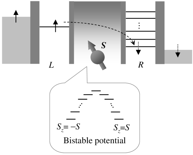
Figure 1: Schematic illustration of “electrode/$L$/spin quantum dot/$R$/electrode” junctions. The $L$ has an energy level of conduction electrons with up-spin, while the $R$ has $N_{\uparrow}$ energy levels of conduction electrons with up-spin and $N_{\downarrow}$, with down-spin. The shaded area in the electrodes represents the region occupied by electrons. The bias voltage (the gate voltage) is applied to the electrodes (the $L$ and the $R$). In addition, the equivalent circuit is shown in Fig. 10.

II.2 Assumptions

On condition that the initial state of the localized spin is $S_{z}$=$-S$, up-spin electrons are sequentially injected from the left electrode into the dot. Eto To describe the sequentially injected electrons, we have the following assumptions: Eto

1. This system exhibits single electron tunneling (SET), SET in which the up-spin electrons are injected from the left electrode into the dot one by one under specific bias and gate voltages [see Sec. VII]. Concretely speaking, when the probability density of the electron becomes 0 at the $L$ and 1 at the $R$, the electron moves into the right electrode and the subsequent electron is injected into the $L$.

   The situation in which the $m$th electron runs in the dot is named as the $m$th process. When the time period of the $m$th process is represented by $\Delta t^{(m)}$, the finish time of the $m$th process, $t_{m}$, is defined by $t_{m}=\sum_{m^{\prime}=1}^{m}\Delta t^{(m^{\prime})}$. Here, $t_{0}$=0 is the initial time.

2. When the transport of the electron is caused by interaction $V$ between the $L$ and the $R$, $V$ acts while each electron runs in the $L$-dot-$R$ system. On the other hand, $V$ is switched off for the electron being outside of this system. The interaction for the $m$th injected electron at time $T$, $V^{(m)}(T)$, is written by,

   $${V}^{(m)}(T)=\left\{\begin{array}[]{ll}{V},&\hskip 14.22636pt{\rm for}~{}t_{m-1}<T\leq t_{m},\\ 0,&\hskip 14.22636pt{\rm for}~{}T\leq t_{m-1},~{}t_{m}<T,\end{array}\right.$$ (3)

   [see Fig. 2]. As found from this $V^{(m)}(T)$, each process is independent.

   The interaction $V$ is given by a transmission term including the exchange interaction between the electron and the localized spin. Appelbaum1 ; Appelbaum2 ; Anderson ; Kim This term is obtained within the second-order perturbation theory based on the weak couplings between the dot and the QWs. The $L$, $R$, and dot parts are described by an unperturbed Hamiltonian, in which the on-site Coulomb energy is considered in the dot. The couplings between the dot and the QWs are perturbation terms. The resultant $V$ is now expanded to a more general system, namely, the anisotropic exchange interaction. Shiba The expression is written by,

   $${V} = V_{0}\displaystyle{\sum_{n\uparrow=1}^{N_{\uparrow}}}\left({c}_{\mbox{\tiny$R_{n\uparrow}$}}^{\dagger}{c}_{\mbox{\tiny$L_{\uparrow}$}}+{c}_{\mbox{\tiny$L_{\uparrow}$}}^{\dagger}{c}_{\mbox{\tiny$R_{n\uparrow}$}}\right)$$ (4)

   $$+J_{\perp}\displaystyle{\sum_{n\downarrow=1}^{N_{\downarrow}}}\left({c}_{\mbox{\tiny$R_{n\downarrow}$}}^{\dagger}{c}_{\mbox{\tiny$L_{\uparrow}$}}{S}_{+}+{c}_{\mbox{\tiny$L_{\uparrow}$}}^{\dagger}{c}_{\mbox{\tiny$R_{n\downarrow}$}}{S}_{-}\right)$$

   $$+J_{z}\displaystyle{\sum_{n\uparrow=1}^{N_{\uparrow}}}\left({c}_{\mbox{\tiny$R_{n\uparrow}$}}^{\dagger}{c}_{\mbox{\tiny$L_{\uparrow}$}}+{c}_{\mbox{\tiny$L_{\uparrow}$}}^{\dagger}{c}_{\mbox{\tiny$R_{n\uparrow}$}}\right){S}_{z}.$$

   Here, $c_{j}$ ($c_{j}^{{\dagger}}$) is the annihilation (creation) operator of an electron of $j$=$L$ or $R_{n\sigma}$, where the suffix $L$ ($R_{n\sigma}$) denotes the level of conduction electrons with up-spin of the $L$ (the $n$th level of conduction electrons with a $\sigma$ spin of the $R$). Furthermore, $V_{0}$ denotes the coefficient for direct tunneling, while $J_{\perp}$ ($J_{z}$) is that for tunneling with a transverse (longitudinal) exchange interaction between the electron and the localized spin. From now on, we call $J_{\perp}$ ($J_{z}$) the exchange integral.

3. The localized spin canted by the electron is not rapidly relaxed and interacts with the subsequently injected electron.

4. The system has the relation of $|E_{L}-E_{R_{n\sigma}}|\ll|V|$, where $E_{L}$ ($E_{R_{n\sigma}}$) denotes the energy level of conduction electrons with the up-spin of the $L$ (the $n$th energy level of conduction electrons with the $\sigma$ spin of the $R$). The energy levels contain the potential due to the gate voltage. Here, the central region in $E_{R_{n\sigma}}$ is located in the vicinity of $E_{L}$. The band width in $E_{R_{n\sigma}}$ is about $2|D|(2S-1)$, with $|D|[S^{2}-(S-1)^{2}]$=$|D|(2S-1)$, where $|D|(2S-1)$ corresponds to the maximum energy that the conduction electron absorbs from the localized spin or gives to the spin for the case of the energy conservation. Consequently, $|E_{L}-E_{R_{n\sigma}}|\ll|V|$ corresponds to $|D|\ll|V|$. Note that the assumption greatly simplifies the calculation [see Sec. III.1].

   As mentioned in Sec. III.1 [also Ref. 24], the above assumption leads to the relation of $\Delta t^{(m)}\ll\hbar/|E_{L}-E_{R_{n\sigma}}|$, where $\hbar$ is the Planck constant $h$ divided by $2\pi$. On the basis of the relation, we investigate the motion of the electron within the $L$-dot-$R$ system using the wave function obtained from the time-dependent Schr$\ddot{\rm o}$dinger equation. In contrast, the Fermi’s golden rule which is a method to investigate the transport property, is applicable for the case of $\Delta t^{(m)}\gg\hbar/|E_{L}-E_{R_{n\sigma}}|$.

   We also note that in a short time period such as $\Delta t^{(m)}$, the total energy becomes uncertain according to the uncertainty relation between time and energy, although the energy can be certainly conserved after enough time has passed. The electrons then exhibit the elastic and the inelastic transports. Such electrons are accepted by some energy levels in the $R$.

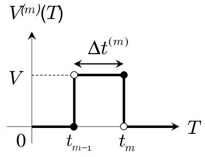
Figure 2: Interaction for the $m$th injected electron in the $m$th process, $V^{(m)}(T)$. Each process is independent.

III Theoretical Formulation

III.1 Wave function

In order to obtain the wave function of the $m$th process, $|\Phi^{(m)}(t)\rangle$ with $t\equiv T-t_{m-1}$ and $0<t\leq\Delta t^{(m)}$, we solve the time-dependent Schr$\ddot{\rm o}$dinger equation,

$$i\hbar\frac{\partial}{\partial t}|\Phi^{(m)}(t)\rangle={\cal H}^{(m)}(t)|\Phi^{(m)}(t)\rangle,$$ (5)

with

$${\cal H}^{(m)}(t)={\cal H}_{0}+V^{(m)}(t),$$ (6)

where ${\cal H}_{0}$ is the Hamiltonian for the electronic states of $L$, $R$, and the localized spin state. The wave function $|\Phi^{(m)}(t)\rangle$ for $0<t\leq\Delta t^{(m)}$ is expressed as,

$$|\Phi^{(m)}(t)\rangle=\displaystyle{\sum_{j}\sum_{S_{z}=-S}^{S}}a_{j,S_{z}}^{(m)}(t)e^{-iE_{j,S_{z}}t/\hbar}|j,S_{z}\rangle,$$ (7)

with

$${\cal H}_{0}|j,S_{z}\rangle=E_{j,S_{z}}|j,S_{z}\rangle,$$ (8)

for $j$=$L$ or $R_{n\sigma}$, and $E_{L,S_{z}}$=$E_{L}-|D|S_{z}^{2}$, $E_{R_{n\sigma},S_{z}}$=$E_{R_{n\sigma}}-|D|S_{z}^{2}$. The state $|L~{}(R_{n\sigma}),S_{z}\rangle$ means that the electron exists at the level of the $L$ (at the $n$th level of the $\sigma$ spin of the $R$) and the localized spin has $S_{z}$. The equation to determine the coefficient $a_{j,S_{z}}^{(m)}(t)$ for $0<t\leq\Delta t^{(m)}$ is given by,

$$\dot{a}_{j,S_{z}}^{(m)}(t) = \displaystyle{\frac{1}{i\hbar}\sum_{k}\sum_{S_{z}^{\prime}=-S}^{S}}\langle j,S_{z}|V|k,S_{z}^{\prime}\rangle a_{k,S_{z}^{\prime}}^{(m)}(t)$$ (9)

$$\times e^{i(E_{j,S_{z}}-E_{k,S_{z}^{\prime}})t/\hbar}.$$

We obtain equations for $a_{L,S_{z}}^{(m)}(t)$, $a_{R_{n\uparrow},S_{z}}^{(m)}(t)$, and $a_{R_{n\downarrow},S_{z}+1}^{(m)}(t)$ using $\langle R_{n\downarrow},S_{z}+1|V|L,S_{z}\rangle=\langle L,S_{z}|V|R_{n\downarrow},S_{z}+1\rangle=J_{\perp}\sqrt{(S-S_{z})(S+S_{z}+1)}\equiv F_{S_{z}}$ and $\langle R_{n\uparrow},S_{z}|V|L,S_{z}\rangle=\langle L,S_{z}|V|R_{n\uparrow},S_{z}\rangle=V_{0}+J_{z}S_{z}\equiv G_{S_{z}}$. Their equations are summarized as follows:

$$\ddot{a}_{L,S_{z}}^{(m)}(t)=-\frac{F_{S_{z}}^{2}}{\hbar^{2}}N_{\downarrow}a_{L,S_{z}}^{(m)}(t)-\frac{G_{S_{z}}^{2}}{\hbar^{2}}N_{\uparrow}a_{L,S_{z}}^{(m)}(t)$$

$$\hskip 45.52458pt+f_{S_{z}}^{(m)}(t)+g_{S_{z}}^{(m)}(t),$$ (10)

$$\dot{a}_{R_{n\downarrow},S_{z}+1}^{(m)}(t)=-i\frac{F_{S_{z}}}{\hbar}a_{L,S_{z}}^{(m)}(t)e^{-i\Delta_{R_{n\downarrow},S_{z}}t/\hbar},$$ (11)

$$\dot{a}_{R_{n\uparrow},S_{z}}^{(m)}(t)=-i\frac{G_{S_{z}}}{\hbar}a_{L,S_{z}}^{(m)}(t)e^{-i\Delta_{R_{n\uparrow},S_{z}}t/\hbar},$$ (12)

with

$$f_{S_{z}}^{(m)}(t)=\frac{F_{S_{z}}}{\hbar^{2}}\sum_{n\downarrow=1}^{N_{\downarrow}}\Delta_{R_{n\downarrow},S_{z}}a_{R_{n\downarrow},S_{z}+1}^{(m)}(t)e^{i\Delta_{R_{n\downarrow},S_{z}}t/\hbar},$$

$$g_{S_{z}}^{(m)}(t)=\frac{G_{S_{z}}}{\hbar^{2}}\sum_{n\uparrow=1}^{N_{\uparrow}}\Delta_{R_{n\uparrow},S_{z}}a_{R_{n\uparrow},S_{z}}^{(m)}(t)e^{i\Delta_{R_{n\uparrow},S_{z}}t/\hbar},$$

$\Delta_{R_{n\downarrow},S_{z}}=E_{L,S_{z}}-E_{R_{n\downarrow},Sz+1}$, and $\Delta_{R_{n\uparrow},S_{z}}=E_{L,S_{z}}-E_{R_{n\uparrow},Sz}$, where the sum $\sum_{n\downarrow}$ ($\sum_{n\uparrow}$) excludes $n\downarrow$ ($n\uparrow$) giving $\Delta_{R_{n\downarrow},S_{z}}$=0 ($\Delta_{R_{n\uparrow},S_{z}}$=0).

According to $|E_{L}-E_{R_{n\sigma}}|\ll|J_{\perp}|$, $|J_{z}|$, and $|V_{0}|$ of Sec. II.2(iv), the present system has the relation of $|\Delta_{R_{n\downarrow},S_{z}}/F_{S_{z}}|\ll 1$ and $|\Delta_{R_{n\uparrow},S_{z}}/G_{S_{z}}|\ll 1$. comment The time average of $|f_{S_{z}}^{(m)}(t)|$ and $|g_{S_{z}}^{(m)}(t)|$ then becomes negligibly small compared to that of the magnitude of the first and second terms on the right-hand side of Eq. (III.1) because the sum in the complex plane is done in addition to this relation and $|a_{R_{n\downarrow},S_{z}+1}^{(m)}(t)|$ and $|a_{R_{n\uparrow},S_{z}}^{(m)}(t)|$ are 1 at maximum. We hence obtain $a_{L,S_{z}}^{(m)}(t)$ from an approximate expression by omitting $f_{S_{z}}^{(m)}(t)$ and $g_{S_{z}}^{(m)}(t)$ from Eq. (III.1).

The assumption for $a_{L,S_{z}}^{(m)}(t)$ of Sec. II.2(i) is concretely defined as follows: under the voltages described in Secs. II.2(i) and VII, as soon as the local probability density at the $L$ of the $m$th injected electron becomes zero, the $m$th electron goes out of the $R$, and the potential for the $m$th electron is then switched off: $V^{(m)}(T)=0$ for $T>t_{m}$. Next, the subsequent $(m+1)$th electron moves from the left electrode to the $L$. The initial condition of the $m$th process is therefore given by,

$$a_{L,S_{z}}^{(m)}(0) = \left[\sum_{n\uparrow=1}^{N_{\uparrow}}\left|\langle R_{n\uparrow},S_{z}|\Phi^{(m-1)}(\Delta t^{(m-1)})\rangle\right|^{2}\right.$$ (14)

$$\left.+\sum_{n\downarrow=1}^{N_{\downarrow}}\left|\langle R_{n\downarrow},S_{z}|\Phi^{(m-1)}(\Delta t^{(m-1)})\rangle\right|^{2}\right]^{1/2}$$

$$\equiv b_{S_{z}}^{(m)},$$

$$\dot{a}_{L,S_{z}}^{(m)}(0) = 0.$$ (15)

Here, $b_{S_{z}}^{(m)}$ is the initial amplitude of the $m$th process with $0\leq b_{S_{z}}^{(m)}\leq 1$. It is represented by using the probability amplitude specified by the final state of the localized spin of the $(m-1)$th process according to Sec. II.2(iii). In particular, $b_{-S}^{(1)}$=1 is apparent due to $S_{z}$=$-S$ at $T$=0. Furthermore, $\dot{a}_{L,S_{z}}^{(m)}(0)$=0 originates from $V^{(m)}(T)$=0 for $T\leq t_{m-1}$ of Eq. (3).

As a result, the coefficients are obtained as follows:

$$a_{L,S_{z}}^{(m)}(t)=b_{S_{z}}^{(m)}\cos(\Omega_{S_{z}}t),$$ (16)

$$a_{R_{n\downarrow},S_{z}+1}^{(m)}(t)=-\frac{iF_{S_{z}}b_{S_{z}}^{(m)}}{\hbar\Omega_{S_{z}}}\sin(\Omega_{S_{z}}t),$$ (17)

$$a_{R_{n\uparrow},S_{z}}^{(m)}(t)=-\frac{iG_{S_{z}}b_{S_{z}}^{(m)}}{\hbar\Omega_{S_{z}}}\sin(\Omega_{S_{z}}t),$$ (18)

with

$$\Omega_{S_{z}}=\frac{\sqrt{N_{\downarrow}F_{S_{z}}^{2}+N_{\uparrow}G_{S_{z}}^{2}}}{\hbar},$$ (19)

for $0<t\leq\Delta t^{(m)}$. Here, $a_{R_{n\downarrow},S_{z}+1}^{(m)}(t)$ and $a_{R_{n\uparrow},S_{z}}^{(m)}(t)$ are obtained by using $a_{L,S_{z}}^{(m)}(t)$ and Eqs. (11) and (12), where $\Delta_{R_{n\downarrow},S_{z}}t/\hbar$ and $\Delta_{R_{n\uparrow},S_{z}}t/\hbar$ are taken as 0 because $t$ is considered to be, at most, several times larger than $1/\Omega_{S_{z}}$ in this study comment1 and further $|\Delta_{R_{n\downarrow},S_{z}}/F_{S_{z}}|\ll 1$ and $|\Delta_{R_{n\uparrow},S_{z}}/G_{S_{z}}|\ll 1$ are introduced as stated earlier.

In fact, the coefficients of Eqs. (16), (17), and (18) correspond to exact expressions for a system of $D$=0 and $\Delta_{R_{n\downarrow},S_{z}}$=$\Delta_{R_{n\uparrow},S_{z}}$=0 ($E_{L}=E_{R_{n\uparrow}}=E_{R_{n\downarrow}}$) obtained under the condition that the initial state of the localized spin is set to be $S_{z}$=$-S$. The use of the coefficients, however, is considered to be valid for the study of the qualitative properties of the present system with $|E_{L}-E_{R_{n\sigma}}|\ll|J_{\perp}|$, $|J_{z}|$, and $|V_{0}|$.

We substitute Eqs. (16), (17), and (18) into Eq. (7). The wave function $|\Phi^{(m)}(t)\rangle$ for $0<t\leq\Delta t^{(m)}$ is finally written as,

$$|\Phi^{(m)}(t)\rangle=\displaystyle{\sum_{S_{z}=-S}^{S}}A_{L,S_{z}}^{(m)}(t)e^{-iE_{L,S_{z}}t/\hbar}|L,S_{z}\rangle$$

$$+\displaystyle{\sum_{n\uparrow=1}^{N_{\uparrow}}}\displaystyle{\sum_{S_{z}=-S}^{S}}A_{R_{n\uparrow},S_{z}}^{(m)}(t)e^{-iE_{R_{n\uparrow},S_{z}}t/\hbar}|R_{n\uparrow},S_{z}\rangle$$

$$+\displaystyle{\sum_{n\downarrow=1}^{N_{\downarrow}}}\displaystyle{\sum_{S_{z}=-S}^{S-1}}A_{R_{n\downarrow},S_{z}+1}^{(m)}(t)e^{-iE_{R_{n\downarrow},S_{z}+1}t/\hbar}|R_{n\downarrow},S_{z}+1\rangle,$$

with $\displaystyle{A_{L,S_{z}}^{(m)}(t)=\frac{a_{L,S_{z}}^{(m)}(t)}{a^{(m)}(t)}}$, $\displaystyle{A_{R_{n\uparrow},S_{z}}^{(m)}(t)=\frac{a_{R_{n\uparrow},S_{z}}^{(m)}(t)}{a^{(m)}(t)}}$, $\displaystyle{A_{R_{n\downarrow},S_{z}+1}^{(m)}(t)=\frac{a_{R_{n\downarrow},S_{z}+1}^{(m)}(t)}{a^{(m)}(t)}}$, where $a^{(m)}(t)$ is the normalization factor,

$$a^{(m)}(t) = \left[\sum_{S_{z}=-S}^{S}\left|a_{L,S_{z}}^{(m)}(t)\right|^{2}+N_{\uparrow}\sum_{S_{z}=-S}^{S}\left|a_{R_{n\uparrow},S_{z}}^{(m)}(t)\right|^{2}\right.$$ (21)

$$\left.+N_{\downarrow}\sum_{S_{z}=-S}^{S-1}\left|a_{R_{n\downarrow},S_{z}+1}^{(m)}(t)\right|^{2}\right]^{1/2}.$$

The local probability densities at the $L$ and the $R$ are given by,

$$\langle\Phi^{(m)}(t)|{\cal L}|\Phi^{(m)}(t)\rangle = \sum_{S_{z}=-S}^{S}\left|A_{L,S_{z}}^{(m)}(t)\right|^{2},$$ (22)

$$\langle\Phi^{(m)}(t)|{\cal R}|\Phi^{(m)}(t)\rangle = N_{\uparrow}\sum_{S_{z}=-S}^{S}\left|A_{R_{n\uparrow},S_{z}}^{(m)}(t)\right|^{2}$$ (23)

$$+N_{\downarrow}\sum_{S_{z}=-S}^{S-1}\left|A_{R_{n\downarrow},S_{z}+1}^{(m)}(t)\right|^{2},$$

respectively, with ${\cal L}\equiv\sum_{S_{z}=-S}^{S}|L,S_{z}\rangle\langle L,S_{z}|$ and ${\cal R}\equiv\sum_{n\uparrow=1}^{N_{\uparrow}}\sum_{S_{z}=-S}^{S}|R_{n\uparrow},S_{z}\rangle\langle R_{n\uparrow},S_{z}|+\sum_{n\downarrow=1}^{N_{\downarrow}}\sum_{S_{z}=-S}^{S-1}|R_{n\downarrow},S_{z}+1\rangle\langle R_{n\downarrow},S_{z}+1|$.

III.2 Number of electrons in the $R$ and the right electrode

On the basis of Eq. (23), we obtain the number of electrons in the $R$ and the right electrode for the $m$th process, $n_{r}^{(m)}(t)$. The expression is written by,

$$n_{r}^{(m)}(t) = (m-1)+N_{\uparrow}\sum_{S_{z}=-S}^{S}\left|A_{R_{n\uparrow},S_{z}}^{(m)}(t)\right|^{2}$$ (24)

$$+N_{\downarrow}\sum_{S_{z}=-S}^{S-1}\left|A_{R_{n\downarrow},S_{z}+1}^{(m)}(t)\right|^{2},$$

for $0<t\leq\Delta t^{(m)}$. The first term in the right-hand side represents the number of electrons which have moved to the right electrode. The second and third terms are $\langle\Phi^{(m)}(t)|{\cal R}|\Phi^{(m)}(t)\rangle$ of Eq. (23). Furthermore, $n_{r}^{(m)}(t)-(m-1)~{}\left[=\langle\Phi^{(m)}(t)|{\cal R}|\Phi^{(m)}(t)\rangle\right]$ is regarded as the expectation value of the position of the $m$th injected electron when the positions of the $L$ and the $R$ are set to be 0 and 1, respectively.

III.3 Electrical current

The electrical current of the $m$th electron, $I^{(m)}(t)$, is defined by $I^{(m)}(t)$=$-en_{e}S_{d}v^{(m)}(t)$, where $v^{(m)}(t)$ is the velocity of the $m$th electron, $e$ ($>$0) is the electric charge, $n_{e}$ is the number density of electrons, and $S_{d}$ is the cross-sectional area of the dot. The velocity, $v^{(m)}(t)$, is obtained from the time differential of the expectation value of the position of the $m$th injected electron. When the positions of the $L$ and the $R$ are defined as 0 and $l$, respectively, $I^{(m)}(t)$ is written as follows:

$$I^{(m)}(t) = -en_{e}S_{d}l\frac{d}{dt}\langle\Phi^{(m)}(t)|{\cal R}|\Phi^{(m)}(t)\rangle$$

$$= \frac{-en_{e}S_{d}l}{\left[a^{(m)}(t)\right]^{2}}\sum_{S_{z}=-S}^{S}\left[b_{S_{z}}^{(m)}\right]^{2}\Omega_{S_{z}}\sin(2\Omega_{S_{z}}t),$$

for $0<t\leq\Delta t^{(m)}$.

III.4 Expectation value of the localized spin

The expectation value of the localized spin of the $m$th process, $\langle S_{z}^{(m)}(t)\rangle$, is obtained by using Eq. (III.1). The expression is given by,

$$\langle S_{z}^{(m)}(t)\rangle = \langle\Phi^{(m)}(t)|{S}_{z}|\Phi^{(m)}(t)\rangle$$ (26)

$$=\sum_{S_{z}=-S}^{S}S_{z}\left|A_{L,S_{z}}^{(m)}(t)\right|^{2}+N_{\uparrow}\sum_{S_{z}=-S}^{S}S_{z}\left|A_{R_{n\uparrow},S_{z}}^{(m)}(t)\right|^{2}$$

$$+N_{\downarrow}\sum_{S_{z}=-S}^{S-1}(S_{z}+1)\left|A_{R_{n\downarrow},S_{z}+1}^{(m)}(t)\right|^{2},$$

for $0<t\leq\Delta t^{(m)}$.

IV Applications

IV.1 Spin-polarized $R$ with only down-spin levels

The spin reversal occurs when the $R$ has energy levels of conduction electrons with only down-spin. In this system, $V$ is described by only the second term in Eq. (4) because of $N_{\uparrow}$=0. Furthermore, $G_{S_{z}}$, $a_{R_{n\uparrow},S_{z}}^{(m)}(t)$, and $A_{R_{n\uparrow},S_{z}}^{(m)}(t)$ are set to be 0.

Figure 3: Time $t$ dependence of the partial probability density of the $m$th process. Here, $|\langle L,S_{z}|\Phi^{(m)}(t)\rangle|^{2}$ ($\sum_{n\downarrow=1}^{N_{\downarrow}}|\langle R_{n\downarrow},S_{z}+1|\Phi^{(m)}(t)\rangle|^{2}$) is shown by a solid (dashed) curve.

We obtain $|\Phi^{(m)}(t)\rangle$ for $0<t\leq\Delta t^{(m)}$ using Eqs. (16), (17), (III.1), and $b_{S_{z}}^{(m)}$= $\delta_{m,S_{z}+S+1}$ which is Eq. (14) for this system. The expression is written by,

$$|\Phi^{(m)}(t)\rangle=\cos(\omega_{S_{z}}t)e^{-iE_{L,S_{z}}t/\hbar}|L,S_{z}\rangle$$

$$-\sum_{n\downarrow=1}^{N_{\downarrow}}\frac{iJ_{\perp}}{\sqrt{N_{\downarrow}}|J_{\perp}|}\sin(\omega_{S_{z}}t)e^{-iE_{R_{n\downarrow},S_{z}+1}t/\hbar}|R_{n\downarrow},S_{z}+1\rangle,$$

with

$$\omega_{S_{z}}=\frac{\left|J_{\perp}\right|\sqrt{N_{\downarrow}(S-S_{z})(S+S_{z}+1)}}{\hbar}.$$ (28)

and $m$=$S_{z}+S+1$ for $S_{z}$=$-S$ - $S-1$. From Eq. (IV.1), the partial probability density is obtained as follows:

$$\left|\langle L,S_{z}|\Phi^{(m)}(t)\rangle\right|^{2}=\cos^{2}(\omega_{S_{z}}t),$$ (29)

$$\sum_{n\downarrow=1}^{N_{\downarrow}}\left|\langle R_{n\downarrow},S_{z}+1|\Phi^{(m)}(t)\rangle\right|^{2}=\sin^{2}(\omega_{S_{z}}t),$$ (30)

with $m$=$S_{z}+S+1$ for $S_{z}$=$-S$ - $S-1$. For $m=S_{z}+S+1$, $\left|\langle L,S_{z}|\Phi^{(m)}(t)\rangle\right|^{2}$ decreases from 1 to 0 and $\sum_{n\downarrow=1}^{N_{\downarrow}}\left|\langle R_{n\downarrow},S_{z}+1|\Phi^{(m)}(t)\rangle\right|^{2}$ increases from 0 to 1 with increasing $t$ [see Fig. 3]. This behavior means that the electron transfers from the $L$ to the $R$ with the spin flip from up to down and the localized spin changes from $S_{z}$ to $S_{z}+1$. Since the $m$th process is finished at $t=\pi/(2\omega_{S_{z}})$, $\Delta t^{(m)}$ is given by,

$$\Delta t^{(m)}=\frac{\pi}{2\omega_{S_{z}}}=\frac{h}{4\left|J_{\perp}\right|\sqrt{N_{\downarrow}(S-S_{z})(S+S_{z}+1)}},$$ (31)

with $m=S_{z}+S+1$ for $S_{z}$=$-S$ - $S-1$. Here, $m=S_{z}+S+1$ for $S_{z}$=$-S$ - $S-1$ represents $m$=1, 2, 3, 4, $\cdot\cdot\cdot$, 2$S$. The spin reversal is thereby achieved after the ($2S$)th process, where $2S$ also corresponds to the total number of injected electrons.

Using Eq. (31), we can obtain the reversal time of the localized spin, $t_{R}$, which is the total time to transform $S_{z}$ from $-S$ to $S$. When $\Delta t^{(m)}$ with $m=S_{z}+S+1$ of Eq. (31) is renamed as $\Delta t_{\mbox{\footnotesize$S_{z}$}}$, $t_{R}$ is simply written by,

$$t_{R} = \displaystyle{\sum_{S_{z}=-S}^{S-1}\Delta t_{\mbox{\footnotesize$S_{z}$}}}$$ (32)

$$= \displaystyle{\sum_{S_{z}=-S}^{S-1}\frac{h}{4\left|J_{\perp}\right|\sqrt{N_{\downarrow}(S-S_{z})(S+S_{z}+1)}}}.$$

Figure 4 shows the $S$ dependence of $t_{R}|J_{\perp}|\sqrt{N_{\downarrow}}/h$. At $S$=1, $t_{R}$ takes $h\sqrt{2}/(4|J_{\perp}|\sqrt{N_{\downarrow}})$. On the condition that $|J_{\perp}|\sqrt{N_{\downarrow}}/h$ is a constant, $t_{R}$ monotonically increases with increasing $S$. This behavior is explained by considering that the spin reversal is caused by injecting $2S$ up-spin electrons into the dot. In the classical spin limit of $S\to\infty$, $t_{R}$ comes close to $h\pi/(4|J_{\perp}|\sqrt{N_{\downarrow}})$ which is obtained by replacing $\sum_{S_{z}=-S}^{S-1}$ with $\lim_{S\to\infty}\int_{-S}^{S-1}dS_{z}$. We thus find that the $t_{R}$ of systems with $S\geq 1$ has the following relation,

$$\frac{h\sqrt{2}}{4|J_{\perp}|\sqrt{N_{\downarrow}}}\leq t_{R}<\frac{h\pi}{4|J_{\perp}|\sqrt{N_{\downarrow}}}.$$ (33)

Furthermore, since this $t_{R}$ is derived under Sec. II.2(iii), we emphasize that the spin reversal is realized when the relaxation time of the localized spin, $\tau$, satisfies the relation of $\tau>t_{R}=\sum_{S_{z}=-S}^{S-1}h/\left[4|J_{\perp}|\sqrt{N_{\downarrow}(S-S_{z})(S+S_{z}+1)}\right]$.

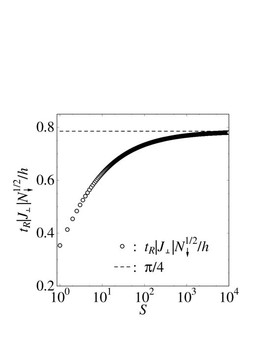
Figure 4: Spin quantum number $S$ dependence of the reversal time of the localized spin, $t_{R}$. Here, $t_{R}|J_{\perp}|\sqrt{N_{\downarrow}}/h$ takes $\sqrt{2}/4$ at $S$=1, while it comes close to $\pi/4$ in the classical spin limit of $S\to\infty$.

As an application, we consider a system with $S$=5, $N_{\downarrow}$=50, and $|J_{\perp}|$=0.001 eV. The reversal time, $t_{R}$, is evaluated to be 3.3 $\times$ 10^-13 s by using Eq. (32). The relation of $\tau>3.3\times 10^{-13}$ s is essential for an experimental observation of this spin reversal.

The upper panel of Fig. 5 shows the $T$ dependence of $n_{r}^{(m)}(T-t_{m-1})$ with $m$=1 - 10. The number of electrons in the $R$ and the right electrode, $n_{r}^{(m)}(T-t_{m-1})$, increases from 0 to 10 with increasing $T$ and becomes 10 at $T=t_{R}=3.3\times 10^{-13}$ s. The reversal is eventually achieved by injecting 10 (=$2S$) electrons into the dot. Furthermore, it is noted that the slope becomes zero at $t_{m}$ with $m$=1 - 9.

The middle panel of Fig. 5 shows the $T$ dependence of $I^{(m)}(T-t_{m-1})/(-en_{e}S_{d}l)$. The quantity $I^{(m)}(T-t_{m-1})/(-en_{e}S_{d}l)$ exhibits a single peak for each process. The peak takes the largest value for the 5th and 6th processes, where the respective initial states have $S_{z}$ = $-$1 and 0. This behavior reflects the fact that $\omega_{S_{z}}$ achieves its maximum at $S_{z}$ = $-$1 and 0 for $S$=5 [see also Eq. (III.3)].

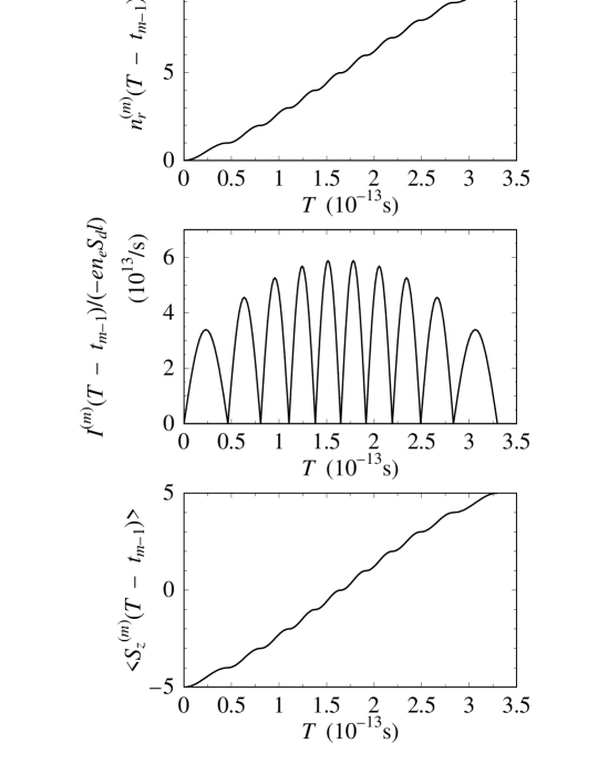
Figure 5: Time $T$ dependence of the number of electrons in the $R$ and the right electrode, $n_{r}^{(m)}(T-t_{m-1})$; electrical current, $I^{(m)}(T-t_{m-1})$; and expectation value of the localized spin, $\langle S_{z}^{(m)}(T-t_{m-1})\rangle$; $m$=1 - 10 for the system of $S$=5, $N_{\downarrow}$=50, and $|J_{\perp}|$=0.001 eV. Upper panel: $n_{r}^{(m)}(T-t_{m-1})$. Middle panel: $I^{(m)}(T-t_{m-1})/(-en_{e}S_{d}l)$. Lower panel: $\langle S_{z}^{(m)}(T-t_{m-1})\rangle$.

The lower panel of Fig. 5 shows the $T$ dependence of $\langle S_{z}^{(m)}(T-t_{m-1})\rangle$. The expectation value of the localized spin $\langle S_{z}^{(m)}(T-t_{m-1})\rangle$ increases from $-$5 to 5 with increasing $T$ following the same pattern as that of $n_{r}^{(m)}(T-t_{m-1})$. It finally becomes 5 at $T=t_{R}=3.3\times 10^{-13}$ s; that is, the spin reversal is completed at this $t_{R}$.

Figure 6: Time $T$ dependence of $n_{r}^{(m)}(T-t_{m-1})$ and $\langle S_{z}^{(m)}(T-t_{m-1})\rangle$ with $m$=1 - 57 for the system of $S$=2 and $N_{\uparrow}$=$N_{\downarrow}$=20. The parameter set of $V$ is $V_{0}$=0.001 eV, $J_{\perp}/V_{0}$=12/31, and $J_{z}/V_{0}=2\sqrt{11}/31$. Upper panel: $n_{r}^{(m)}(T-t_{m-1})$. Lower panel: $\langle S_{z}^{(m)}(T-t_{m-1})\rangle$.

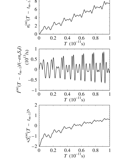
Figure 7: Time $T$ dependence of $n_{r}^{(m)}(T-t_{m-1})$, $I^{(m)}(T-t_{m-1})/(-en_{e}S_{d}l)$, and $\langle S_{z}^{(m)}(T-t_{m-1})\rangle$ with $m$=1 - 8 for the system of $S$=2 and $N_{\uparrow}$=$N_{\downarrow}$=20. The parameter set of $V$ is the same as that of Fig. 6. Upper panel: $n_{r}^{(m)}(T-t_{m-1})$. Middle panel: $I^{(m)}(T-t_{m-1})/(-en_{e}S_{d}l)$. Lower panel: $\langle S_{z}^{(m)}(T-t_{m-1})\rangle$. Here, $n_{r}^{(m)}(T-t_{m-1})$ and $\langle S_{z}^{(m)}(T-t_{m-1})\rangle$ are the respective ones on the larger scale of Fig. 6.

IV.2 Non-magnetic $R$

In the case of non-magnetic $R$ with $N_{\uparrow}$=$N_{\downarrow}$, this system exhibits spin reversal or non-reversal depending on the exchange integral.

Regarding the spin reversal, all injected electrons can transfer from the $L$ to the $R$; that is, the local probability density at the $L$ becomes zero at a certain time for each process [see Sec. II.2(i)]. We therefore pay attention to the local probability density at the $L$ of the $m$th process,

$$\langle\Phi^{(m)}(t)|{\cal L}|\Phi^{(m)}(t)\rangle\propto\displaystyle{\sum_{S_{z}=-S}^{S}}\left[b_{S_{z}}^{(m)}\right]^{2}\cos^{2}(\Omega_{S_{z}}t),$$ (34)

which is obtained from Eqs. (16) and (22). Equation (34) becomes zero at $t=\Delta t^{(m)}$, when $\Delta t^{(m)}$ satisfies the following relation,

$$\Omega_{S_{z}}\Delta t^{(m)}=\left(n_{S_{z}}^{(m)}+\frac{1}{2}\right)\pi,$$ (35)

for any $S_{z}$ giving finite $b_{S_{z}}$. Here, $n_{S_{z}}^{(m)}$ $(\geq 0)$ is the counting number.

In the first process with $b_{-S}^{(1)}$=1, Eq. (34) becomes $\cos^{2}(\Omega_{-S}t)$, and it certainly takes zero at $t=\Delta t^{(1)}=\pi/(2\Omega_{-S})$. In the $m$th process with $m\geq 2$, $b_{S_{z}}^{(m)}$ is finite for any $S_{z}$. Whether Eq. (35) is satisfied for $m\geq 2$ or not depends on the parameter set of the exchange integral.

Table 1: Initial amplitude of the $m$th process, $b_{S_{z}}^{(m)}$; counting number of the $m$th process, $n_{S_{z}}^{(m)}$; and time period of the $m$th process, $\Delta t^{(m)}$ for the system of $S$=2, $N_{\uparrow}$=$N_{\downarrow}$=20, $V_{0}$=0.001 eV, $J_{\perp}/V_{0}$=12/31, and $J_{z}/V_{0}=2\sqrt{11}/31$.

$m$	$b_{-2}^{(m)}$	$b_{-1}^{(m)}$	$b_{0}^{(m)}$	$b_{1}^{(m)}$	$b_{2}^{(m)}$	$\Delta t^{(m)}$
	$n_{-2}^{(m)}$	$n_{-1}^{(m)}$	$n_{0}^{(m)}$	$n_{1}^{(m)}$	$n_{2}^{(m)}$
1	1	0	0	0	0	$\displaystyle{\frac{\pi}{2\Omega_{-2}}}$
	0	0	0	0	0
2	0.47	0.88	0	0	0	$\displaystyle{\frac{3\pi}{2\Omega_{-2}}}$
	1	2	0	0	0
3	0.22	0.79	0.57	0	0	$\displaystyle{\frac{3\pi}{2\Omega_{-2}}}$
	1	2	3	0	0
4	0.10	0.64	0.72	0.26	0	$\displaystyle{\frac{3\pi}{2\Omega_{-2}}}$
	1	2	3	4	0
5	0.50 $\times 10^{-1}$	0.50	0.76	0.41	0.73$\times 10^{-1}$	$\displaystyle{\frac{3\pi}{2\Omega_{-2}}}$
	1	2	3	4	5
$\cdot$	$\cdot$	$\cdot$	$\cdot$	$\cdot$	$\cdot$	$\cdot$
$\cdot$	$\cdot$	$\cdot$	$\cdot$	$\cdot$	$\cdot$	$\cdot$
$\cdot$	$\cdot$	$\cdot$	$\cdot$	$\cdot$	$\cdot$	$\cdot$
30	0.38 $\times 10^{-9}$	0.65 $\times 10^{-3}$	0.58$\times 10^{-1}$	0.44	0.90	$\displaystyle{\frac{3\pi}{2\Omega_{-2}}}$
	1	2	3	4	5
$\cdot$	$\cdot$	$\cdot$	$\cdot$	$\cdot$	$\cdot$	$\cdot$
$\cdot$	$\cdot$	$\cdot$	$\cdot$	$\cdot$	$\cdot$	$\cdot$
$\cdot$	$\cdot$	$\cdot$	$\cdot$	$\cdot$	$\cdot$	$\cdot$
57	0.67 $\times 10^{-18}$	0.50$\times 10^{-6}$	0.26$\times 10^{-2}$	0.14	0.99	$\displaystyle{\frac{3\pi}{2\Omega_{-2}}}$
	1	2	3	4	5

We first investigate the parameter set satisfying Eq. (35) in order to find the spin reversal. For a system with $S$=2 and $N_{\uparrow}$=$N_{\downarrow}$=20, the parameter set is, for example, $V_{0}$=0.001 eV, $J_{\perp}/V_{0}$=12/31, $J_{z}/V_{0}=2\sqrt{11}/31$. In Table 1, we summarize $b_{S_{z}}^{(m)}$, $n_{S_{z}}^{(m)}$, and $\Delta t^{(m)}$ for each $m$. The first process with $b_{-2}^{(1)}$=1 has $\Delta t^{(1)}=\pi/(2\Omega_{-2})=4.78\times 10^{-13}$ s, and the $m$th process with $m\geq 2$ has $\Delta t^{(m)}=3\pi/(2\Omega_{-2})=1.43\times 10^{-12}$ s.

The upper panel of Fig. 6 and the upper panel of Fig. 7 show the $T$ dependence of $n_{r}^{(m)}(T-t_{m-1})$ with the above parameter set in the regions of $0\leq T\leq 8\times 10^{-11}$ s and $0\leq T\leq 1\times 10^{-11}$ s, respectively. Here, $T=8\times 10^{-11}$ s ($T=1\times 10^{-11}$ s) corresponds to the time in the 57th (8th) process. The number of electrons in the $R$ and the right electrode, $n_{r}^{(m)}(T-t_{m-1})$, slightly oscillates in each process and clearly increases with increasing $T$. In the middle panel of Fig. 7, it is shown that $I^{(m)}(T-t_{m-1})/(-en_{e}S_{d}l)$ oscillates between positive and negative values

The lower panel of Fig. 6 and the lower panel of Fig. 7 show the $T$ dependence of $\langle S_{z}^{(m)}(T-t_{m-1})\rangle$ in the respective regions of $T$. The expectation value of the localized spin, $\langle S_{z}^{(m)}(T-t_{m-1})\rangle$, has a slight oscillation in each process as well. The spin reversal is almost realized in the vicinity of $T=8.0\times 10^{-11}$ s, and it is also confirmed from $b_{2}^{(57)}=0.99$ in Table 1.

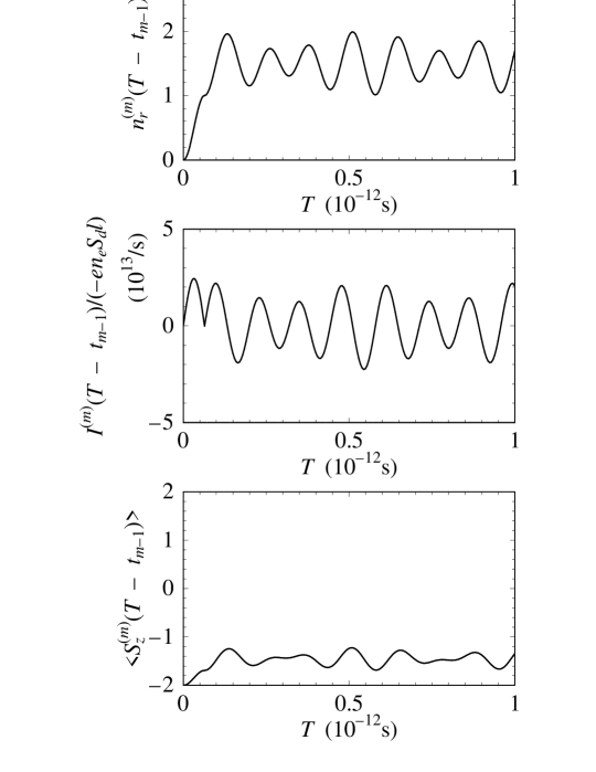
Figure 8: Time $T$ dependence of $n_{r}^{(m)}(T-t_{m-1})$, $I^{(m)}(T-t_{m-1})/(-en_{e}S_{d}l)$, and $\langle S_{z}^{(m)}(T-t_{m-1})\rangle$ with $m$=1, 2 for the system of $S$=2 and $N_{\uparrow}$=$N_{\downarrow}$=20. The parameter set of $V$ is $V_{0}$=0.001 eV, $J_{\perp}/V_{0}$=1, and $J_{z}/V_{0}=2$. Upper panel: $n_{r}^{(m)}(T-t_{m-1})$. Middle panel: $I^{(m)}(T-t_{m-1})/(-en_{e}S_{d}l)$. Lower panel: $\langle S_{z}^{(m)}(T-t_{m-1})\rangle$.

As the spin non-reversal case for $S$=2 and $N_{\uparrow}$=$N_{\downarrow}$=20, we choose, for example, the parameter set of $V_{0}$=0.001 eV, $J_{\perp}/V_{0}$=1, $J_{z}/V_{0}$=2, which does not have $t$ to satisfy Eq. (35) for $S_{z}=-2,-1,0,1,2$. In the first process with $b_{-2}^{(1)}$=1, Eq. (34) becomes $\left|\langle\Phi^{(1)}(t)|{\cal L}|\Phi^{(1)}(t)\rangle\right|^{2}\propto\cos^{2}(\Omega_{-2}t)$ and it takes zero at $t=\pi/(2\Omega_{-2})$=$6.4\times 10^{-14}$ s. In fact, the first injected electron is transferable as seen from the upper panel of Fig. 8. In the second process, Eq. (34) always has finite values. The second injected electron is trapped in the dot and it oscillates between the $L$ and the $R$ as shown in the upper and middle panels of Fig. 8. The localized spin also oscillates between $S_{z}$=$-2$ and $S_{z}$=$-1$ [see the lower panel of Fig. 8].

In addition, we report that qualitative behaviors identical to those noted above are found for some systems (some $S$’s).

V Comments

What follows is a comment about an application of the system with the non-magnetic $R$. According to the present study, the system exhibits a spin reversal or non-reversal depending on the exchange integral. The exchange integral is originally described by the orbital energy level and the on-site Coulomb energy in the dot and transfer integrals between the dot and the QWs. Schrieffer Thereby, by controlling the orbital energy level with the application of the gate voltage, this system may be switchable between the spin reversal and the spin non-reversal.

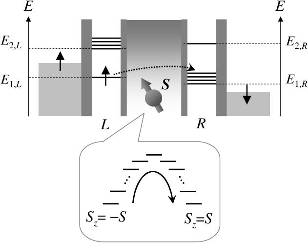
(a)

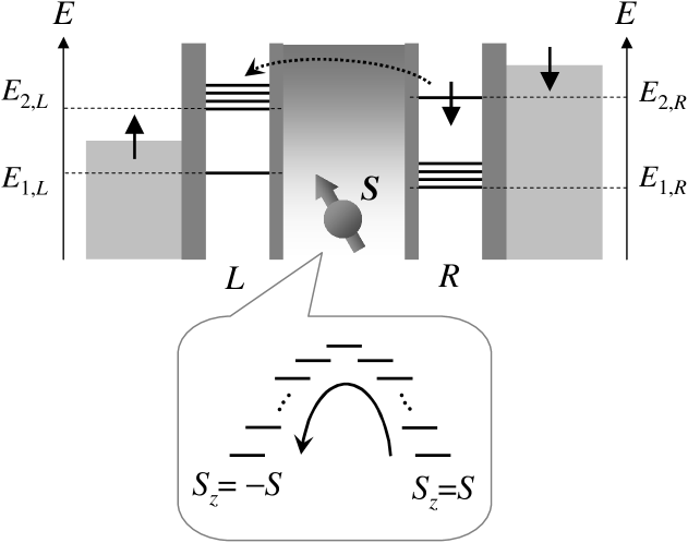
(b)

Figure 9: A model with reversible switching between $S_{z}$=$-S$ and $S$. (a) The reversal from $S_{z}$=$-S$ to $S$ is induced by injecting the up-spin electrons from the $L$ into the dot. (b) The reversal from $S_{z}$=$S$ to $-S$ is achieved by injecting the down-spin electrons from the $R$ into the dot.

Secondly, we propose a model with reversible switching between $S_{z}$=$-S$ and $S$ [see Fig. 9]. The $L$ has energy levels of conduction electrons with up-spin, in which an energy level is located at $E_{1,L}$ and the lowest of the $N_{\uparrow}^{\prime}$ energy levels is found at $E_{2,L}$. The $R$ has levels of conduction electrons with down-spin, in which a level is located at $E_{2,R}$ and the lowest of the $N_{\downarrow}$ levels lies at $E_{1,R}$. Here, tunneling probabilities between the level at $E_{1,L}$ of the $L$ and that at $E_{2,R}$ of the $R$ and between the levels in the vicinity of $E_{2,L}$ of the $L$ and those in the vicinity of $E_{1,R}$ of the $R$ are assumed to be negligibly small. The energy of the highest occupied state (i.e. the Fermi level) of the right electrode is changed by applying the bias voltage, while that of the left electrode is fixed between $E_{1,L}$ and $E_{2,L}$. It should be noted that some electrons lying between the energy of the highest occupied state of the left electrode and that of the right electrode contribute to the transport.

We now consider the SET regime as described in Sec. VII. When the bias voltage is applied to the right electrode as shown in Fig. 9 (a), the up-spin electrons are injected from the $L$ into the dot and the reversal from $S_{z}$=$-S$ to $S$ can be induced through the interaction of Eq. (4) with ${N_{\uparrow}}$=0. On the other hand, in the vicinity of $E_{2,R}$, the interaction between the electron and the localized spin is written by,

$$V=J_{\perp}^{\prime}\displaystyle{\sum_{n\uparrow=1}^{N_{\uparrow}^{\prime}}}\left({c}_{\mbox{\tiny$R_{\downarrow}$}}^{\dagger}{c}_{\mbox{\tiny$L_{n\uparrow}$}}{S}_{+}+{c}_{\mbox{\tiny$L_{n\uparrow}$}}^{\dagger}{c}_{\mbox{\tiny$R_{\downarrow}$}}{S}_{-}\right),$$ (36)

where the suffix $R_{\downarrow}$ ($L_{n\uparrow}$) denotes the level of conduction electrons with the down-spin of the $R$ (the $n$th level of conduction electrons with the up-spin of the $L$), and $J_{\perp}^{\prime}$ is the transverse exchange integral between the localized spin and the electron in this energy region. When the bias voltage is applied to the right electrode as shown in Fig. 9 (b), the down-spin electrons are injected from the $R$ into the dot and the reversal from $S_{z}$=$S$ to $-S$ is achieved through the interaction of Eq. (36).

Finally, we discuss the experimental aspects from the viewpoint of the magnitude of current density. In the case of $S$=5, $N_{\downarrow}$=50, and $|J_{\perp}|$=0.001 eV, the required maximum current density for the spin reversal, $j_{\mbox{\tiny max}}$, is evaluated to be $j_{\mbox{\tiny max}}$= $I_{\mbox{\tiny max}}/S_{d}$ $\simeq$ 4.2 $\times$ 10⁸ A/cm², where the maximum current $I_{\mbox{\tiny max}}$ is given by $I_{\mbox{\tiny max}}$ = $(5.9\times 10^{13})\times(1.6\times 10^{-19})$ $\simeq$ 9.4 $\times$ 10^-6 A as shown in the middle panel of Fig. 5, with $n_{e}S_{d}l$=1 and $e$=$1.6\times 10^{-19}$ C. Furthermore, $S_{d}$ is set to be $S_{d}$=(1.5 $\times$ 10^-7)² cm², which is obtained by assuming that the molecule with $S$=5 has a cubic structure that is about 1.5 nm per side. This length is roughly estimated using examples from a similar molecule, Mn₁₂ with $S$=10. Sessoli In terms of sustainability, the abovementioned $j_{\mbox{\tiny max}}$ is high for typical ferromagnetic tunnel junctions, such as CoFeB/MgO/CoFeB junctions with critical current densities for the MRSI of 7.8 $\times$ 10⁵ A/cm² and 1.2 $\times$ 10⁷ A/cm². Hayakawa1 On the other hand, it has been recently reported that some carbon nanotubes can individually carry currents with density exceeding $10^{9}$ A/cm². CNT1 ; CNT2 We therefore anticipate that appropriate use of carbon nanotubes encapsulating magnetic molecules CNT_mag will lead to the achievement of the spin reversal. In addition, we strongly believe that the current density can be tuned by controlling the exchange integral and $N_{\uparrow}$ (or $N_{\downarrow}$), as found from Eq. (III.3). Namely, the current density decreases with reducing the magnitude of the exchange integral and $N_{\uparrow}$ (or $N_{\downarrow}$).

VI Conclusion

We studied the localized quantum spin reversal for a case in which up-spin electrons were sequentially injected into the spin quantum dot. To describe the sequentially injected electrons, we first made assumptions about the sequential injection of spins and then proposed a simple method based on approximate solutions from the time-dependent Schr$\ddot{\rm o}$dinger equation. This method was applied to systems with the following $R$; that is, (a) the spin-polarized $R$ having energy levels of conduction electrons with only down-spin, and (b) the non-magnetic $R$. The respective results are summarized below.

1. The system exhibited a spin reversal. In particular, we derived the expression of the reversal time of the localized spin and explicitly showed the upper and lower limits of this time for systems with $S\geq 1$. In addition, analytic expressions for the expectation value of the localized spin and the electrical current were obtained as a function of time.

2. The system of $S$=2 and $N_{\uparrow}$=$N_{\downarrow}$=20 exhibited the spin reversal or non-reversal depending on the exchange integral. In the spin non-reversal case, the second injected electron was trapped in the dot, although all injected electrons transferred from the $L$ to the $R$ for the spin reversal case.

We expect that the above-described phenomena will be observed with the advancement of experimental techniques and will be utilized in spin electronics devices in the future.

VII Appendix: bias and gate voltages for the SET

The SET region in the plane of the bias and gate voltages for the model of Fig. 1 is found. We investigate the energy change $\Delta E$ which is obtained by subtracting the energy of the initial charge state from that of the final charge state. The change of state really occurs for $\Delta E<0$.

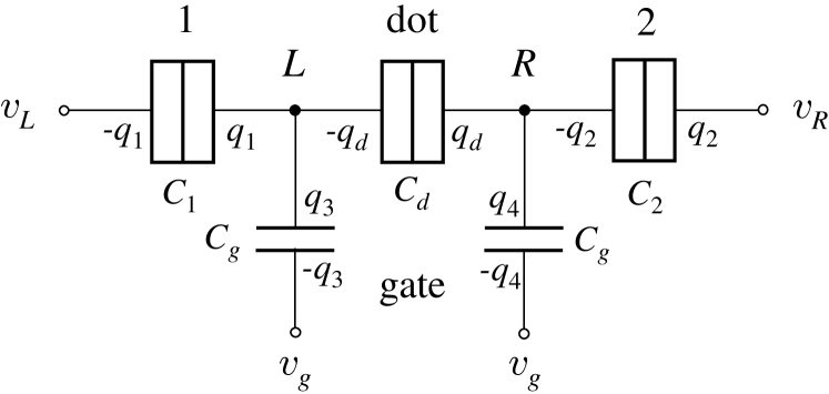
Figure 10: Equivalent circuit for “electrode/$L$/spin quantum dot/$R$/electrode” junctions. The tunnel barrier between the left electrode and the $L$ (between the $R$ and the right electrode) is named 1 (2). Each symbol composed of two rectangles represents both the condenser and the tunnel junctions which enable electron tunneling to take place. Each condenser of the gate is assumed to have a thick barrier that suppresses the electron tunneling.

The equivalent circuit for this model is shown in Fig. 10. The bias voltage of the left electrode (the right electrode) is represented by $v_{L}$ ($v_{R}$), and the voltage of the gate electrode is $v_{g}$. The capacitances of junctions of 1, 2, the dot, and the gate are $C_{1}$, $C_{2}$, $C_{d}$, and $C_{g}$, respectively. The electric charge of the respective junctions is $q_{i}$ ($i$=1-4, $d$).

When the initial charge at the $L$ ($R$) is represented by $q_{L}$ ($q_{R}$), the final charge at the $L$ ($R$) is $q_{L}^{\prime}$ ($q_{R}^{\prime}$), and the change of the charge number in the left electrode (right electrode) is $\Delta n_{Le}$ ($\Delta n_{Re}$), the energy change $\Delta E_{q_{L},q_{R},q_{L}^{\prime},q_{R}^{\prime},\Delta n_{Le},\Delta n_{Re}}$ is given by,

$$\Delta E_{q_{L},q_{R},q_{L}^{\prime},q_{R}^{\prime},\Delta n_{Le},\Delta n_{Re}}=\Delta U-W_{1}-W_{2}-W_{3}-W_{4},$$

where $\Delta U$ denotes the change of the electrostatic energy, and $W_{1}$ ($W_{2}$) represents the work done by the voltage of the left electrode (the right electrode) and $W_{3}$ ($W_{4}$) is that of the left gate electrode (the right gate electrode). These expressions are written as follows:

$$\Delta U=U^{\prime}-U,$$ (38)

$$U=\frac{C_{1}}{2}(\phi_{L}-v_{L})^{2}+\frac{C_{2}}{2}(v_{R}-\phi_{R})^{2}+\frac{C_{d}}{2}(\phi_{R}-\phi_{L})^{2}$$

$$\hskip 25.6073pt+\frac{C_{g}}{2}(\phi_{L}-v_{g})^{2}+\frac{C_{g}}{2}(\phi_{R}-v_{g})^{2},$$ (39)

$$U^{\prime}=\frac{C_{1}}{2}(\phi_{L}^{\prime}-v_{L})^{2}+\frac{C_{2}}{2}(v_{R}-\phi_{R}^{\prime})^{2}+\frac{C_{d}}{2}(\phi_{R}^{\prime}-\phi_{L}^{\prime})^{2}$$

$$\hskip 25.6073pt+\frac{C_{g}}{2}(\phi_{L}^{\prime}-v_{g})^{2}+\frac{C_{g}}{2}(\phi_{R}^{\prime}-v_{g})^{2},$$ (40)

$$W_{1}=-\Delta q_{1}v_{L}-e\Delta n_{Le}v_{L},$$ (41)

$$W_{2}=\Delta q_{2}v_{R}+e\Delta n_{Re}v_{R},$$ (42)

$$W_{3}=-\Delta q_{3}v_{g},$$ (43)

$$W_{4}=-\Delta q_{4}v_{g},$$ (44)

with

$$\Delta q_{1}=C_{1}(\phi_{L}^{\prime}-v_{L})-C_{1}(\phi_{L}-v_{L}),$$ (45)

$$\Delta q_{2}=C_{2}(v_{R}-\phi_{R}^{\prime})-C_{2}(v_{R}-\phi_{R}),$$ (46)

$$\Delta q_{3}=C_{g}(\phi_{L}^{\prime}-v_{g})-C_{g}(\phi_{L}-v_{g}),$$ (47)

$$\Delta q_{4}=C_{g}(\phi_{R}^{\prime}-v_{g})-C_{g}(\phi_{R}-v_{g}),$$ (48)

$$\phi_{L}=\alpha q_{R}+\beta q_{L}+\gamma,$$ (49)

$$\phi_{R}=\zeta q_{R}+\alpha q_{L}+\eta,$$ (50)

$$\phi_{L}^{\prime}=\alpha q_{R}^{\prime}+\beta q_{L}^{\prime}+\gamma,$$ (51)

$$\phi_{R}^{\prime}=\zeta q_{R}^{\prime}+\alpha q_{L}^{\prime}+\eta,$$ (52)

$$\alpha=\frac{C_{d}}{X},$$ (53)

$$\beta=\frac{1}{X}(C_{2}+C_{d}+C_{g}),$$ (54)

$$\gamma=\frac{1}{X}\left[C_{d}(C_{2}v_{R}+C_{g}v_{g})\right.$$

$$\hskip 25.6073pt\left.+(C_{2}+C_{d}+C_{g})(C_{1}v_{L}+C_{g}v_{g})\right],$$ (55)

$$\zeta=\frac{1}{X}(C_{1}+C_{d}+C_{g}),$$ (56)

$$\eta=\frac{1}{X}\left[C_{d}(C_{1}v_{L}+C_{g}v_{g})\right.$$

$$\hskip 25.6073pt\left.+(C_{1}+C_{d}+C_{g})(C_{2}v_{R}+C_{g}v_{g})\right],$$ (57)

$$X=(C_{1}+C_{d}+C_{g})(C_{2}+C_{d}+C_{g})-C_{d}^{2},$$ (58)

where $e$ ($>$0) is the electric charge. The works, $-e\Delta n_{Le}v_{L}$ of Eq. (41) and $e\Delta n_{Re}v_{R}$ of Eq. (42) represent that the electrodes are provided with the changed portion of the charge due to the tunnel electron. Further, $\phi_{L}$ ($\phi_{R}$) is the electrostatic potential of the $L$ ($R$), and Eqs. (49) and (50) are obtained from the following equations,

$$q_{L}=-q_{d}+q_{1}+q_{3},$$ (59)

$$q_{R}=-q_{2}+q_{d}+q_{4},$$ (60)

with $q_{1}$=$C_{1}(\phi_{L}-v_{L})$, $q_{2}$=$C_{2}(v_{R}-\phi_{R})$, $q_{3}$=$C_{g}(\phi_{L}-v_{g})$, $q_{4}$=$C_{g}(\phi_{R}-v_{g})$, $q_{d}$=$C_{d}(\phi_{R}-\phi_{L})$. The bias voltage $v_{L}$ ($v_{R}$) is now set to be $-v/2$ ($v/2$). When $\Delta E_{q_{L},q_{R},q_{L}^{\prime},q_{R}^{\prime},\Delta n_{Le},\Delta n_{Re}}$=0, the relation between $v$ and $v_{g}$ is given by,

$$v=\frac{-\left[\lambda(d_{1}-d_{3})+\nu(d_{2}+d_{3})\right]v_{g}-d_{4}}{\kappa(d_{1}-d_{3})+\mu(d_{2}+d_{3})-\frac{1}{2}(\Delta n_{Re}+\Delta n_{Le})e},$$ (61)

with

$$d_{1}=(C_{1}+C_{g})\left[\alpha(q_{R}^{\prime}-q_{R})+\beta(q_{L}^{\prime}-q_{L})\right],$$ (62)

$$d_{2}=(C_{2}+C_{g})\left[\zeta(q_{R}^{\prime}-q_{R})+\alpha(q_{L}^{\prime}-q_{L})\right],$$ (63)

$$d_{3}=C_{d}\left[(\zeta-\alpha)(q_{R}^{\prime}-q_{R})+(\alpha-\beta)(q_{L}^{\prime}-q_{L})\right],$$

(64)

$$d_{4}=\frac{C_{2}+C_{g}}{2}\left[-(\zeta q_{R}+\alpha q_{L})^{2}+(\zeta q_{R}^{\prime}+\alpha q_{L}^{\prime})^{2}\right]$$

$$\hskip 25.6073pt+\frac{C_{1}+C_{g}}{2}\left[(\alpha q_{R}^{\prime}+\beta q_{L}^{\prime})^{2}-(\alpha q_{R}+\beta q_{L})^{2}\right]$$

$$\hskip 25.6073pt+\frac{C_{d}}{2}\left\{\left[(\zeta-\alpha)q_{R}^{\prime}+(\alpha-\beta)q_{L}^{\prime}\right]^{2}\right.$$

$$\hskip 25.6073pt\left.-\left[(\zeta-\alpha)q_{R}+(\alpha-\beta)q_{L}\right]^{2}\right\},$$ (65)

$$\kappa=\frac{1}{2X}(C_{2}C_{d}-C_{1}C_{2}-C_{1}C_{d}-C_{1}C_{g}),$$ (66)

$$\lambda=\frac{1}{X}(C_{2}C_{g}+2C_{d}C_{g}+C_{g}^{2}),$$ (67)

$$\mu=\frac{1}{2X}(C_{1}C_{2}+C_{2}C_{d}+C_{2}C_{g}-C_{1}C_{d}),$$ (68)

$$\nu=\frac{1}{X}(C_{1}C_{g}+2C_{d}C_{g}+C_{g}^{2}).$$ (69)

This model exhibits the SET under the specific $v$ and $v_{g}$, which satisfy $\Delta E_{0,0,-e,0,1,0}<0$, $\Delta E_{-e,0,0,-e,0,0}<0$, $\Delta E_{0,-e,0,0,0,1}<0$, $\Delta E_{0,-e,-e,-e,1,0}>0$, and $\Delta E_{0,0,0,+e,0,1}>0$. In Fig. 11, the SET region for a system with $C_{1}$=$C_{2}$, $C_{d}$=10$C_{1}$, and $C_{g}$=$0.1C_{1}$ is shown by the shaded area.

We furthermore describe the present transport property; that is, when the probability density of the injected electron becomes 0 at the $L$ and 1 at the $R$, the electron moves into the right electrode, while the electron cannot go to the right electrode if the probability density is finite for both the $L$ and the $R$. This property is based on the following two assumptions: First, there is no direct transfer integral between the $L$ and the right electrode. Second, the wave function extended over both the $R$ and the right electrode can be ignored, although that extended over both the $L$ and the $R$ is taken into account, under the condition that the coupling between the $R$ and the right electrode is much smaller than that between the $L$ and the $R$, i.e. Eq. (4).

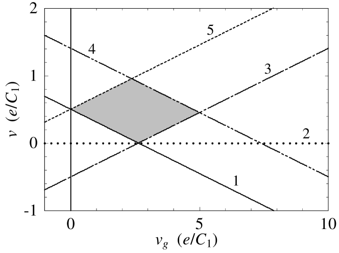
Figure 11: SET region in the bias ($v$) and gate ($v_{g}$) voltage plane for the equivalent circuit with $v_{L}$=$-v/2$, $v_{R}$=$v/2$, $C_{1}$=$C_{2}$, $C_{d}$=10$C_{1}$, and $C_{g}$=$0.1C_{1}$. This region is shown by the shaded area which satisfies $\Delta E_{0,0,-e,0,1,0}<0$, $\Delta E_{-e,0,0,-e,0,0}<0$, $\Delta E_{0,-e,0,0,0,1}<0$, $\Delta E_{0,-e,-e,-e,1,0}>0$, and $\Delta E_{0,0,0,+e,0,1}>0$. The meaning of each line is as follows: 1: $\Delta E_{0,0,-e,0,1,0}$=0, 2: $\Delta E_{-e,0,0,-e,0,0}$=0, 3: $\Delta E_{0,-e,0,0,0,1}$=0, 4: $\Delta E_{0,-e,-e,-e,1,0}$=0, 5: $\Delta E_{0,0,0,+e,0,1}$=0, where the expression is given by Eq. (61).

References

- (1) J. C. Slonczewski, J. Magn. Magn. Mater. 159, L1 (1996).
- (2) L. Berger, Phys. Rev. B 54, 9353 (1996).
- (3) C. Heide, P. E. Zilberman, and R. J. Elliott, Phys. Rev. B 63, 64424 (2001).
- (4) S. Zhang, P. M. Levy, and A. Fert, Phys. Rev. Lett. 88, 236601 (2002).
- (5) E. B. Myers, D. C. Ralph, J. A. Katine, R. N. Louie, and R. A. Buhrman, Science 285, 867 (1999).
- (6) J. Hayakawa, H. Takahashi, K. Ito, M. Fujimori, S. Heike, T. Hashizume, M. Ichimura, S. Ikeda, and H. Ohno, J. Appl. Phys. 97, 114321 (2005).
- (7) Y. Suzuki, A. Tulapurkar, K. Yagami, T. Devolder, A. Fukushima, K. Akio, H. Kubota, S. Yuasa, P. Crozat, and C. Chappert, Jpn. J Appl. Phys. 45, 3842 (2006).
- (8) T. Ochiai, Y. Jiang, A. Hirohata, N. Tezuka, S. Sugimoto, and K. Inomata, Appl. Phys. Lett. 86, 242506 (2005).
- (9) J. A. Katine, F. J. Albert, R. A. Buhrman, E. B. Myers, and D. C. Ralph, Phys. Rev. Lett. 84, 3149 (2000).
- (10) J. Grollier, V. Cros, A. Hamzic, J. M. George, H. Jaffres, A. Fert, G. Faini, J. Ben Youssef, and H. Legall, Appl. Phys. Lett. 78, 3663 (2001).
- (11) A. Caneschi, D. Gatteschi, and R. Sessoli, J. Am. Chem. Soc. 113, 5873 (1991).
- (12) R. Sessoli, H.-L. Tsai, A. R. Schake, S. Wang, J. B. Vincent, K. Folting, D. Gatteschi, G. Christou, and D. N. Hendrickson, J. Am. Chem. Soc. 115, 1804 (1993).
- (13) L. Thomas, F. Lionti, R. Ballou, D. Gatteschi, R. Sessoli, and B. Barbara, Nature 383, 145 (1996).
- (14) F. Luis, J. Bartolome, and J. F. Fernndez, Phys. Rev. B 57, 505 (1998).
- (15) J. Villain, F. Hartman-Boutron, R. Sessoli, and A. Rettori, Europhys. Lett. 27, 159 (1994).
- (16) K. Takeda and K. Awaga, Phys. Rev. B 56, 14560 (1997); K. Takeda, K. Awaga, and T. Inabe, Phys. Rev. B 57, R11062 (1998).
- (17) For example, see M. Eto, T. Ashiwa, and M. Murata, J. Phys. Soc. Jpn. 73, 307 (2004).
- (18) For example, see K. K. Likharev, IBM J. Res. Dev. 32, 144 (1988).
- (19) J. Appelbaum, Phys. Rev. Lett. 17, 91 (1966).
- (20) J. Appelbaum, Phys. Rev. 154, 633 (1967).
- (21) P. W. Anderson, Phys. Rev. Lett. 17, 95 (1966).
- (22) G.-H. Kim and T.-S. Kim, Phys. Rev. Lett. 92, 137203 (2004).
- (23) H. Shiba, J. Phys. Soc. Jpn. 43, 601 (1970).
- (24) As for the spin-polarized , by using Eq. (31), is found to correspond to [see Sec. II.2(iv)]. For the non-magnetic , and are related to by taking into account in Table 1.
- (25) In the case of spin reversal of non-magnetic , corresponds to in Table 1 at maximum, which is times as large as . In the case of spin-polarized , is Eq. (31) at maximum, which is times as large as .
- (26) J. R. Schrieffer and P. A. Wolff, Phys. Rev. 149, 491 (1966).
- (27) J. Hayakawa, S. Ikeda, Y. M. Lee, R. Sasaki, T. Meguro, F. Matsukura, H. Takahashi, and H. Ohno, Jpn. J. Appl. Phys. 44, L1267 (2005).
- (28) Z. Yao, C. L. Kane, and C. Dekker, Phys. Rev. Lett. 84, 2941 (2000).
- (29) B. Q. Wei, R. Vajtai, and P. M. Ajayan, Appl. Phys. Lett. 79, 1172 (2001).
- (30) For example, see X. X. Zhang, G. H. Wen, S. Huang, L. Dai, R. Gao, and Z. L. Wang, J. Magn. Magn. Mater. 231, L9 (2001); X. Zhao, S. Inoue, M. Jinno, T. Suzuki, and Y. Ando, Chem. Phys. Lett. 373, 266 (2003); S. Kokado and K. Harigaya, J. Phys.: Condens. Matter 16, 5605 (2004).