Numerical study of a multiscale expansion of the Korteweg de Vries equation and Painlevé-II equation

Abstract.

The Cauchy problem for the Korteweg de Vries (KdV) equation with small dispersion of order $\epsilon^{2}$, $\epsilon\ll 1$, is characterized by the appearance of a zone of rapid modulated oscillations. These oscillations are approximately described by the elliptic solution of KdV where the amplitude, wave-number and frequency are not constant but evolve according to the Whitham equations. Whereas the difference between the KdV and the asymptotic solution decreases as $\epsilon$ in the interior of the Whitham oscillatory zone, it is known to be only of order $\epsilon^{1/3}$ near the leading edge of this zone. To obtain a more accurate description near the leading edge of the oscillatory zone we present a multiscale expansion of the solution of KdV in terms of the Hastings-McLeod solution of the Painlevé-II equation. We show numerically that the resulting multiscale solution approximates the KdV solution, in the small dispersion limit, to the order $\epsilon^{2/3}$.

1. Introduction

The mathematically rigorous study of the small dispersion limit of the Korteweg de Vries (KdV) equation

(1.1) $$u_{t}+6uu_{x}+\epsilon^{2}u_{xxx}=0,\quad\epsilon\ll 1,$$

with smooth initial data $u_{0}(x)$ was initiated in the works of Lax-Levermore [28], which stimulated intense research both numerically and analytically on the problem.

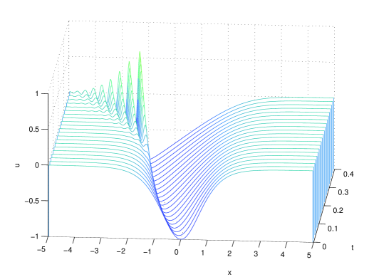
Figure 1. Numerical solution of the KdV equation for the initial data $u_{0}(x)=-\mbox{sech}^{2}x$ and $\epsilon=0.1$.

The solution of the Cauchy problem of the KdV equation in the small dispersion limit is characterized by the appearance of a zone of rapid oscillations of frequency of order $1/\epsilon$, see for instance Fig. 1.

These oscillations are formed in the strong nonlinear regime and they have been analytically described in terms of elliptic functions, and in the general case in terms of theta functions in [34], [8]; the evolution in time of the oscillations was studied in [30]. These results give a good asymptotic description of the oscillations only near the center of the oscillatory zone (see Fig. 2).

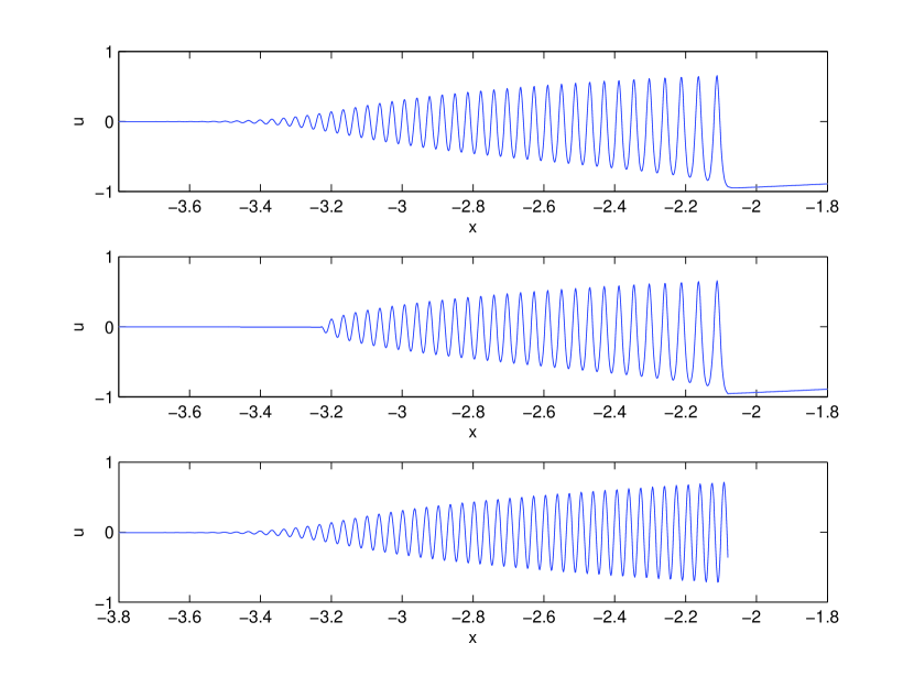
Figure 2. We plot for $u_{0}=-\mbox{sech}^{2}x$, $t=0.4$ and $\epsilon=10^{-2}$ from top to bottom: 1) the numerical solution of KdV; 2) the asymptotic formula (2.3) in terms of elliptic functions and the Hopf solution; 3) the multiscale solution where the envelope of the oscillations is given by a solution to the Painlevé-II equation.

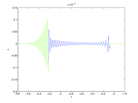
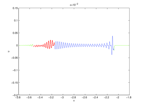
Figure 3. In (a) the difference between the upper two plots of Fig. 2 is shown. The Whitham zone is shown in blue. In (b) one can see the same situation as in (a) except for the region close to the leading edge of the Whitham zone where the difference between the KdV and the multiscale solution is shown in red.

In [19] we have studied numerically the small dispersion limit of the KdV equation for the concrete example of initial data of the form

(1.2) $$u_{0}(x)=-\mbox{sech}^{2}x.$$

We have compared the asymptotic description given in the works [28, 34, 8] with the numerical KdV solution. In [19] we have shown numerically that the difference between the KdV solution and the elliptic asymptotic solution at the center of the oscillatory zone scales like $\epsilon$ while this fails to be true at the boundary of the oscillatory zone. This fact was also observed for the Benjamin-Ono in [24]. In particular at the left boundary, where the amplitude of the oscillations tend to zero, the difference between the KdV solution and the elliptic asymptotic solution scales like $\epsilon^{\frac{1}{3}}$. In this manuscript we show that the Painlevé-II equation describes the envelope of the oscillations at the leading edge where the oscillations tend to zero. More precisely

$$u(x,t,\epsilon)=u(t)+\epsilon^{1/3}a\cos\left(\frac{\psi}{\epsilon}\right)+O(\epsilon^{2/3})$$

where $u(t)=u(x^{-}(t),t)$ solve the Hopf equation at the boundary $x^{-}(t)$ of the oscillatory zone, $\psi$ is a phase determined in (3.29) and $a$ is, up to shift and rescalings, the Hastings-McLeod solution of Painlevè-II equation

$$A_{zz}=zA+2A^{3}$$

with boundary conditions

$$\lim_{z\rightarrow-\infty}A(z)=\sqrt{-z/2},\quad\lim_{z\rightarrow+\infty}A(z)=\mbox{Ai}(z)$$

where $\mbox{Ai}(z)$ is the Airy function.

Painlevé equations appear in many branches of mathematics (for a review see [6]). For example in the study of self-similar solutions of integrable equations, in the study of the Hele-Shaw flow near singularities [14], or in double-scaling limits in random matrix models (see e.g. [1], [15],[2],[5]). In this work, following [27], we perform a double-scaling limit of the KdV equation to derive the asymptotic description of the leading edge oscillations which are formed in the KdV small dispersion limit. We show that the envelope of the oscillations is determined by the Hastings-McLeod [22] solution of the Painlevé-II equation. Then we compare numerically for the initial data $u_{0}(x)=-\mbox{sech}^{2}x$ at the leading edge of the oscillatory front, the KdV solution with the derived multiscale solution and show that the difference between the two solutions scales like $\epsilon^{\frac{2}{3}}$. We identify a neighborhood of the leading edge of the Whitham zone where the multiscale solution gives a better asymptotic description than the asymptotic solution based on the elliptic and the Hopf solution. This allows to patch different asymptotic descriptions to provide a more satisfactory treatment of the small dispersion limit of KdV as shown in Fig. 3.
Our analytical investigation of the multiscale expansion of the KdV solution requires the following assumptions on the initial data:

• $u_{0}(x)$ is negative with a single minimum; we chose the minimum to be at $x=0$ and normalized to -1, namely $u_{0}(0)=-1$;

• the function $f_{-}(u)$ which is the inverse of the monotone decreasing part of the initial data $u_{0}(x)$ is such that $f^{\prime\prime\prime}_{-}(u)<0$;

• $\int_{-\infty}^{+\infty}u_{0}(x)(1+x^{2})dx<\infty$.

The last condition guarantees that the solution of the Cauchy problem for KdV exists for all times $t>0$.

This manuscript is organized as follows. In section 2 we review the small dispersion limit of the KdV equation and study the small amplitude limit of the oscillations. In section 3 we perform a multiscale expansion of the KdV solution when the oscillations tend to zero, and we show that the envelope of the oscillations is given by a solution of the Painlevé-II equation. In section 4 we numerically compare the KdV solution with the multiscale solution obtained in section 2. We show that the difference between the two solutions scales as $\epsilon^{\frac{2}{3}}$ which is in accordance with our analytical result. We identify a zone near the leading edge where the multiscale solution provides a better description than the elliptic and the Hopf solution and patch the solutions. In section 5 we summarize the results and add some concluding remarks on future directions of research.

2. Asymptotic solution of KdV in the small dispersion limit

The solution of the Cauchy problem for the KdV equation is characterized by the appearance of a zone of fast oscillations of wave-length of order $\epsilon$, see e.g. Fig. 1. These oscillations were called by Gurevich and Pitaevski dispersive shock waves [21]. Following the work of [28], [34] and [8], the description of the small dispersion limit of the KdV equation is the following:
1) for $0\leq t<t_{c}$, where $t_{c}$ is a critical time, the solution $u(x,t,\epsilon)$ of the KdV Cauchy problem is approximated, for small $\epsilon$, by $u(x,t)$ which solves the Hopf equation

(2.1) $$u_{t}+6uu_{x}=0.$$

Here $t_{c}$ is the time when the first point of gradient catastrophe appears in the solution

(2.2) $$u(x,t)=u_{0}(\xi),\quad x=6tu_{0}(\xi)+\xi,$$

of the Hopf equation. From the above, the time $t_{c}$ of gradient catastrophe can be evaluated from the relation

$$t_{c}=\dfrac{1}{\max_{\xi\in\mathbb{R}}[-6u_{0}^{\prime}(\xi)]}.$$

2) After the time of gradient catastrophe, the solution of the KdV equation is characterized by the appearance of an interval of rapid modulated oscillations. According to the Lax-Levermore theory, the interval $[x^{-}(t),x^{+}(t)]$ of the oscillatory zone is independent of $\epsilon$. Here $x^{-}(t)$ and $x^{+}(t)$ are determined from the initial data and satisfy the condition $x^{-}(t_{c})=x^{+}(t_{c})=x_{c}$ where $x_{c}$ is the $x$-coordinate of the point of gradient catastrophe of the Hopf solution. Outside the interval $[x^{-}(t),x^{+}(t)]$ the leading order asymptotics of $u(x,t,\epsilon)$ as $\epsilon\rightarrow 0$ is described by the solution of the Hopf equation (2.2). Inside the interval $[x^{-}(t),x^{+}(t)]$ the solution $u(x,t,\epsilon)$ is approximately described, for small $\epsilon$, by the elliptic solution of KdV [21], [28], [34], [8],

(2.3) $$u(x,t,\epsilon)\simeq+\beta_{1}+\beta_{2}+\beta_{3}+2\alpha+2\epsilon^{2}\frac{\partial^{2}}{\partial x^{2}}\log\theta(\Omega(x,t);\mathcal{T})$$

where

(2.4) $$\Omega=\dfrac{\sqrt{\beta_{1}-\beta_{3}}}{2\epsilon K(s)}[x-2t(\beta_{1}+\beta_{2}+\beta_{3})-q]$$

and

(2.5) $$\alpha=-\beta_{1}+(\beta_{1}-\beta_{3})\frac{E(s)}{K(s)},\;\;\mathcal{T}=i\dfrac{K^{\prime}(s)}{K(s)},\;\;s^{2}=\frac{\beta_{2}-\beta_{3}}{\beta_{1}-\beta_{3}}$$

with $K(s)$ and $E(s)$ the complete elliptic integrals of the first and second kind, $K^{\prime}(s)=K(\sqrt{1-s^{2}})$; $\theta$ is the Jacobi elliptic theta function defined by the Fourier series

(2.6) $$\theta(z;\mathcal{T})=\sum_{n\in\mathbb{Z}}e^{\pi in^{2}\mathcal{T}+2\pi inz}.$$

For constant values of the $\beta_{i}$ the formula (2.3) is an exact solution of KdV well known in the theory of finite gap integration [23], [10]. However in the description of the leading order asymptotics of $u(x,t,\epsilon)$ as $\epsilon\rightarrow 0$, the quantities $\beta_{i}$ depend on $x$ and $t$ and evolve according to the Whitham equations [35]

(2.7) $$\dfrac{\partial}{\partial t}\beta_{i}+v_{i}\dfrac{\partial}{\partial x}\beta_{i}=0,\quad i=1,2,3,$$

where the speeds $v_{i}$ are given by the formula

(2.8) $$v_{i}=4\frac{\prod_{k\neq i}(\beta_{i}-\beta_{k})}{\beta_{i}+\alpha}+2(\beta_{1}+\beta_{2}+\beta_{3}),$$

with $\alpha$ as in (2.5). The formula for $q$ in the phase $\Omega$ in (2.4) that we are giving below was introduced in [19] and looks different but is equivalent to the one in [8]

(2.9) $$q(\beta_{1},\beta_{2},\beta_{3})=\frac{1}{2\sqrt{2}\pi}\int_{-1}^{1}\int_{-1}^{1}d\mu d\nu\frac{f_{-}(\frac{1+\mu}{2}(\frac{1+\nu}{2}\beta_{1}+\frac{1-\nu}{2}\beta_{2})+\frac{1-\mu}{2}\beta_{3})}{\sqrt{1-\mu}\sqrt{1-\nu^{2}}},$$

where $f_{-}(y)$ is the inverse function of the decreasing part of the initial data $u_{0}$. The above formula for $q(\beta_{1},\beta_{2},\beta_{3})$ is valid as long as $\beta_{1}>\beta_{2}>\beta_{3}>-1$. When $\beta_{3}$ reaches the minimum value $-1$ and passes over the negative hump, it is necessary to take into account also the increasing part of the initial data $f_{+}(u)$ in formula (2.9). We denote by $T$ this time. For $t>T>t_{c}$ we introduce the variable $X_{3}$ defined by $u_{0}(X_{3})=\beta_{3}$ which is still monotonous. For values of $X_{3}$ beyond the hump, namely $X_{3}>0$, we have to substitute (2.9) by the formula

(2.10) $$q(\beta_{1},\beta_{2},\beta_{3})=\frac{1}{\sqrt{2}\pi}\int_{\beta_{2}}^{\beta_{1}}d\lambda\dfrac{\left(\int_{\beta_{3}}^{-1}d\mu\frac{f_{+}(\mu)}{\sqrt{\lambda-\mu}}+\int_{-1}^{\lambda}\frac{f_{-}(\mu)}{\sqrt{\lambda-\mu}}\right)}{\sqrt{(\beta_{1}-\lambda)(\lambda-\beta_{2})(\lambda-\beta_{3})}}.$$

The function $q=q(\beta_{1},\beta_{2},\beta_{3})$ is symmetric with respect to $\beta_{1},\beta_{2}$ and $\beta_{3}$, and satisfies a linear over-determined system of Euler-Poisson-Darboux type. It has been introduced in the work of Fei-Ran Tian [30]. The Whitham equations (2.7) can be integrated through the so called hodograph transform, which generalizes the method of characteristics, and which gives the solution in the implicit form [33]

(2.11) $$x=v_{i}t+w_{i},\quad i=1,2,3,$$

where the $v_{i}$ are defined in (2.8) and the $w_{i}=w_{i}(\beta_{1},\beta_{2},\beta_{3})$ are obtained from an algebro-geometric procedure [26] by the formula [30]

(2.12) $$w_{i}=\frac{1}{2}\left(v_{i}-2\sum_{k=1}^{3}\beta_{k}\right)\frac{\partial q}{\partial\beta_{i}}+q,\quad i=1,2,3,$$

with $q$ defined in (2.9) or (2.10). Formula (2.11) solves the initial value problem for the Whitham equations (2.7) with boundary conditions:
a) leading edge:

(2.13) $$\begin{split}&\beta_{1}=\mbox{ the Hopf solution (\ref{Hopf})}\\ &\beta_{2}=\beta_{3},\end{split}$$

b) trailing edge:

(2.14) $$\begin{split}&\beta_{2}=\beta_{1}\\ &\beta_{3}=\mbox{ the Hopf solution (\ref{Hopf})}.\end{split}$$

In [19] we have solved numerically the initial value problem for the Whitham equations. In this way we could perform a numerical comparison between the KdV small dispersion solution and the asymptotic formula (2.3) (see Fig. 3). While in the interior of the oscillatory zone the error scales numerically like $\epsilon$, at the left boundary of the oscillatory zone the error scales numerically like $\epsilon^{\frac{1}{3}}$. To derive a more satisfactory asymptotic approximation of the KdV small dispersion limit in the vicinity of this point, we perform in the next section a double scaling expansion of the KdV equation, following the double scaling limits appearing in random matrix theory. Before doing this analysis, we study the elliptic solution (2.3) in the limit when the oscillations go to zero.

2.1. Small amplitude limit of the elliptic solution

We study the elliptic solution (2.3) near the leading edge, namely when oscillations go to zero. To avoid degeneracies, we rewrite the system (2.11) in the equivalent form

(2.15) $$\left\{\begin{aligned} &(v_{1}t+w_{1}-x)(\alpha+\beta_{1})=0\\ &v_{2}t+w_{2}-x=0\\ &\dfrac{1}{(\beta_{2}-\beta_{3})}[(v_{2}-v_{3})t+w_{2}-w_{3}]=0.\end{aligned}\right.$$

and perform the limit $\delta\rightarrow 0$ where

$$\beta_{2}=v+\delta,\quad\beta_{3}=v-\delta,\quad\beta_{1}=u.$$

To simplify our calculation we restrict ourselves to the case $t_{c}<t<T$. The following limit holds:

(2.16) $$\dfrac{E(s)}{K(s)}=1-\dfrac{\delta}{v-\beta_{1}}+\dfrac{3}{4}\dfrac{\delta^{2}}{(v-\beta_{1})^{2}}+O(\delta^{3})$$

such that

(2.17) $$\alpha=-v-\dfrac{\delta^{2}}{4(u-v)}.$$

Furthermore the following identities hold

(2.18) $$f_{-}(u)= [2(u-v)\partial_{u}q(u,v,v)+q(u,v,v)]$$

(2.19) $$\Phi(v,u)= \partial_{v}q(u,v,v)+\partial_{u}q(u,v,v)$$

where

(2.20) $$\Phi(v,u)=\frac{1}{2\sqrt{2}}\int_{-1}^{1}d\mu\frac{f^{\prime}_{-}(\frac{1+\mu}{2}v+\frac{1-\mu}{2}u)}{\sqrt{1-\mu}}=\frac{1}{2\sqrt{v-u}}\int_{u}^{v}d\mu\frac{f^{\prime}_{-}(\mu)}{\sqrt{v-\mu}}.$$

Substituting (2.17) (2.18) and (2.19) into (2.15) we arrive at the system

(2.21) $$\left\{\begin{aligned} x&=6tu+f_{-}(u)-\delta^{2}\dfrac{(x-6tu-f_{-}(u)-2(u-v)(6t+\Phi(v;u))}{8(v-u)^{2}}+O(\delta^{4}),\\ x&=6tu+f_{-}(u)+2(v-u)[6t+\Phi(v,u)]+\delta[6t+\Phi(v,u)+(v-u)\partial_{v}\Phi(v,u)]\\ &+\dfrac{\delta^{2}}{4(u-v)}[6t-2(u-v)^{2}\partial_{vvv}q(u,v,v)+4(u-v)\partial_{vv}q(u,v,v)+\dfrac{3}{2}\partial_{v}q(u,v,v,)]+O(\delta^{3})\\ 0&=6t+\Phi(v,u)+(v-u)\partial_{v}\Phi(v,u)+O(\delta).\end{aligned}\right.$$

From the above we deduce that, in the limit $\delta\rightarrow 0$, the hodograph transform (2.15) reduces to the form (see [30][18])

(2.22) $$\left\{\begin{aligned} &6ut+f_{-}(u)-x=0\\ &\Phi(v,u)+6t=0\\ &\partial_{v}\Phi(v,u)=0.\end{aligned}\right.$$

The above system enables one to determine $x$, $u$ and $v$ as a function of time. This time dependence will be denoted $x=x^{-}(t)$, $u=u(t)$ and $v=v(t)$. We are interested in studying the behavior of the elliptic solution (2.3) near the leading edge, namely when $x-x^{-}(t)$ is small and $x>x^{-}(t)$. For this purpose we introduce two unknown functions of $x$ and $t$,

$$\delta=\delta(x-x^{-}(t)),\quad\Delta=\Delta(x-x^{-}(t))$$

which tend to zero as $x\rightarrow x^{-}(t)$. We are going to derive the dependence of $\Delta$ as a function of $x-x^{-}(t)$. Let us fix

(2.23) $$\beta_{2}=v+\delta,\quad\beta_{3}=v-\delta,\;\;\delta\rightarrow 0\quad\beta_{1}=u+\Delta,\;\;\Delta\rightarrow 0.$$

Using the first equation of (2.21) we obtain

$$0=x-6tu-f_{-}(\beta_{1})+\delta^{2}\dfrac{(x-6t\beta_{1}-f_{-}(\beta_{1})-2(\beta_{1}-v)(6t+\Phi(v;\beta_{1}))}{8(\beta_{3}-u)^{2}}+O(\delta^{4}).$$

Expanding the above expression near $\beta_{1}(x,t)=u(t)+\Delta(x,t)$, using the identity

(2.24) $$\dfrac{\partial}{\partial\beta_{1}}\Phi(\beta_{3};\beta_{1})=\dfrac{\Phi(\beta_{3};\beta_{1})-\Phi(\beta_{1};\beta_{1})}{2(\beta_{3}-\beta_{1})}$$

and (2.22) we arrive at the expression

(2.25) $$0\simeq x-x^{-}(t)-(6t+f^{\prime}_{-}(u))\Delta+\dfrac{\delta^{2}}{8(v-u)^{2}}(x-x^{-}(t)),$$

so that

(2.26) $$\Delta\simeq\dfrac{x-x^{-}(t)}{6t+f^{\prime}_{-}(u)}.$$

Using the second equation in (2.21) we arrive at

(2.27) $$x-x^{-}(t)\simeq\delta^{2}\,c$$

where

(2.28) $$\begin{split}c&=[6t-2(u-v)^{2}\partial_{vvv}q(u,v,v)+4(u-v)\partial_{vv}q(u,v,v)+\dfrac{3}{2}\partial_{v}q(u,v,v,)]/4(u-v)\\ &=-\dfrac{u-v}{2}\partial_{vv}\Phi(v;u).\end{split}$$

Therefore

$$\dfrac{\delta^{2}}{\Delta}=O(1).$$

Theorem 2.1.

The elliptic solution (2.3) in the limit (2.23) takes the form

(2.29) $$u(x,t,\epsilon)\simeq u(t)+\dfrac{x-x^{-}(t)}{6t+f^{\prime}_{-}(u)}+2\delta\cos\left(2\pi\dfrac{\Omega^{-}}{\epsilon}\right)+\delta^{2}\dfrac{\cos\left(4\pi\dfrac{\Omega^{-}}{\epsilon}\right)-1}{2(u(t)-v(t))},$$

where the phase $\Omega^{-}$ takes the form

(2.30) $$2\pi\Omega^{-}=\phi_{0}+\phi_{2}$$

with

(2.31) $$\phi_{0}(t)=-16\int_{t_{c}}^{t}(u(\tau)-v(\tau))^{\frac{3}{2}}d\tau,\;\;\;\phi_{2}(x,t)=2\sqrt{u(t)-v(t)}(x-x^{-}(t)),$$

and $u(t)$, $v(t)$ and $x^{-}(t)$ solve the system (2.22).

Proof.

We first prove the relation (2.30). Using the expansion

$$K(s)=\dfrac{\pi}{2}\left(1+\dfrac{s^{2}}{4}+\dfrac{9}{64}s^{4}+O(s^{6})\right),\quad$$

and (2.18) we obtain the following limit for the phase $\Omega$ in (2.4)

$$2\pi\Omega|_{\beta_{2,3}=v\pm\delta} =2\sqrt{\beta_{1}-v}(1-\dfrac{3\delta^{2}}{16(\beta_{1}-v)^{2}})[x-6t\beta_{1}-f_{-}(\beta_{1})$$

$$+2(\beta_{1}-v)(2t+\partial_{\beta_{1}}q(\beta_{1},v,v)-\dfrac{\delta^{2}}{4}\partial^{2}_{v}q(\beta_{1},v,v)]+O(\delta^{4}).$$

Using the identity

$$\partial_{v}^{2}q(\beta_{1},v,v)=\partial_{v}\Phi(v,\beta_{1})-\partial_{\beta_{1}}\partial_{v}q(\beta_{1},v,v),$$

(2.22) and (2.19) we can rewrite the above in the form

$$\partial_{v}^{2}q(\beta_{1},v,v)=\dfrac{3(2t+\partial_{\beta_{1}}q(\beta_{1},v,v))}{2(v-\beta_{1})}+\dfrac{3}{4}\dfrac{6t+f^{\prime}_{-}(u)}{(v-u)^{2}}\Delta+O(\Delta^{2})$$

so that the phase $\Omega$ takes the form

(2.32) $$2\pi\Omega|_{\beta_{2,3}=v\pm\delta}\simeq 4(\beta_{1}-v)^{\frac{3}{2}}(2t+\partial_{\beta_{1}}q(\beta_{1},v,v))-\dfrac{\delta^{2}}{8}\dfrac{x-x^{-}(t)}{(v-u)^{\frac{3}{2}}}.$$

We define

$$\eta_{0}(\beta_{1},v):= 4\sqrt{\beta_{1}-v}[2(\beta_{1}-v)t+(\beta_{1}-v)\partial_{\beta_{1}}q(\beta_{1},v,v)]$$

(2.33) $$= 2\int_{v}^{\beta_{1}}\sqrt{\beta_{1}-\lambda}[\Phi(\lambda,\beta_{1})+6t]d\lambda,$$

so that, expanding near $\beta_{1}=u+\Delta$, by (2.22)

(2.34) $$\begin{split}\eta_{0}(\beta_{1},v)=\eta_{0}(u,v)+\phi_{2}(x,t)+O(\Delta^{2}),\end{split}$$

where $\phi_{2}(x,t)$ is defined in (2.31). To show that $\eta_{0}(u,v)$ defined in (2.33) coincides with $\phi_{0}$ defined in (2.31), we differentiate (2.33) with respect to time,

$$2\dfrac{d}{dt}\int_{v}^{u}\sqrt{u-\lambda}[\Phi(\lambda,u)+6t]d\lambda=-16(u-v)^{\frac{3}{2}}$$

where we have used the identity (2.24) and $\partial_{t}u(t)=12\dfrac{(v-u)}{6t+f^{\prime}_{-}(u)}.$ Integrating the r.h.s of the above expression with respect to $t$ from $t_{c}$ to $t$ we obtain the formula (2.31).

Using (2.34) and (2.26) we rewrite the phase (2.32) in the form

(2.35) $$2\pi\Omega|_{\begin{subarray}{c}\beta_{1}=u+\Delta\\ \beta_{2,3}=v\pm\delta\end{subarray}}=\phi_{0}+\phi_{2}-\dfrac{\delta^{2}(x-x^{-}(t))}{8(u-v)^{\frac{3}{2}}}+O(\Delta^{2})$$

where $\phi_{0}$ and $\phi_{2}$ are as in (2.31). Neglecting the higher order terms in $\delta$ and $\Delta$ of the above expansion one obtains (2.30).

Now we are ready to expand the theta-function expression in the limit of small amplitudes. Using (2.17) and

$$e^{i\pi\mathcal{T}}=\dfrac{\delta}{8(u-v)}(1-\frac{\Delta}{u-v})+\dfrac{5}{128}\dfrac{\delta^{2}}{(u-v)^{3}}+O(\delta^{5},\delta^{3}\Delta),$$

one derives the small amplitude limit of the Jacobi $\theta$-function (2.6)

$$\theta(z;\tau)=1+\dfrac{\delta}{4(u-v)}(1-\frac{\Delta}{u-v})\cos(2\pi z)+O(\delta^{4}).$$

Substituting the above expansion in (2.3) one obtains

$$u(x,t,\epsilon)\simeq u(t)+\dfrac{x-x^{-}(t)}{6t+f^{\prime}_{-}(u)}+2\delta(x,t)\cos\left(2\pi\dfrac{\Omega^{-}}{\epsilon}\right)+\delta(x,t)^{2}\dfrac{\cos\left(4\pi\dfrac{\Omega^{-}}{\epsilon}\right)-1}{2(u(t)-v(t))}.$$

which coincides with (2.29). ∎

3. Painlevé equations at the leading edge

In this section we present a multiscale description of the oscillatory behavior of a solution to the KdV equation in the small dispersion limit close to the leading edge $x^{-}(t)$ where $\beta_{2}=\beta_{3}=v$ and $\beta_{1}=u$. We are interested in the double scaling limit to the solution of the KdV equation (1.1) as $\epsilon\rightarrow 0$ and $x\rightarrow x^{-}(t)$ in such a way that $x-x^{-}(t)\propto\epsilon^{2/3}$. We introduce the rescaled coordinate $y$ near the leading edge,

(3.1) $$y=\epsilon^{-2/3}(x-x^{-}(t)),$$

which transforms the KdV equation (1.1), to the form

(3.2) $$\epsilon^{\frac{2}{3}}u_{t}+\epsilon^{\frac{2}{3}}u_{yyy}+(6u-x^{-}_{t})u_{y}=0,$$

where $x^{-}_{t}=\dfrac{d}{dt}x^{-}(t)$. The substitution (3.1) has the effect that the linear term of (3.2) is just the Airy equation $u_{t}+u_{yyy}=0$ which has oscillatory solutions.

It is known [9],[27] that the corrections to the Hopf solution near the leading edge are of the order $\epsilon^{1/3}$. We thus make the ansatz

(3.3) $$u(y,t,\epsilon)=U_{0}+\epsilon^{1/3}U_{1}+\epsilon^{2/3}U_{2}+\epsilon U_{3}+\ldots,$$

where $U_{0}=u(t)$ is the solution at the leading edge. We assume that $U_{k\geq 1}$ contains oscillatory terms with oscillations of the order $1/\epsilon$. In particular

(3.4) $$U_{1}=a(y,t)\cos\left(\frac{\psi(y,t)}{\epsilon}\right),$$

where

(3.5) $$\psi(y,t)=\psi_{0}(y,t)+\epsilon^{1/3}\psi_{1}(y,t)+\epsilon^{2/3}\psi_{2}(y,t)+\epsilon\psi_{3}(y,t)+\ldots.$$

Similarly we put

(3.6) $$U_{2}=b_{1}(y,t)+b_{2}(y,t)\cos\left(\frac{2\psi(y,t)}{\epsilon}\right),$$

and

(3.7) $$U_{3}=c_{0}(y,t)+c_{2}(y,t)\sin\left(\frac{2\psi(y,t)}{\epsilon}\right)+c_{3}(y,t)\cos\left(\frac{3\psi(y,t)}{\epsilon}\right).$$

Terms proportional to $\sin(\psi/\epsilon)$ can be absorbed by a redefinition of $\psi$. Since we impose no further restrictions on $\psi$ here, such terms are therefore omitted in all orders. We only consider terms proportional to $\cos(\psi/\epsilon)$ in order $\epsilon^{1/3}$ and the necessary terms in higher order to compensate the terms due to the nonlinearities in (3.2).

If we enter equation (1.1) with this ansatz, we immediately obtain from the term of order $\epsilon^{0}$ that $\psi_{0,y}=\psi_{1,y}=0$. From the term of order $\epsilon^{\frac{1}{3}}$ we get

(3.8) $$\psi_{2,y}^{3}-(6U_{0}-x^{-}_{t})\psi_{2,y}-\psi_{0,t}=0.$$

In order $\epsilon^{2/3}$ we obtain the following equations

(3.9) $$b_{2}-\frac{a^{2}}{2\psi_{2,y}^{2}}=0$$

(3.10) $$\psi_{3,y}(3\psi_{2,y}^{2}-6U_{0}+x^{-}_{t})-\psi_{1,t}=0$$

(3.11) $$\dfrac{d}{dy}[a^{2}(3\psi_{2,y}^{2}-6U_{0}+x^{-}_{t})]=0.$$

In order $\epsilon$ we get

(3.12) $$U_{0,t}+(6U_{0}-x^{-}_{t})b_{1,y}+3aa_{y}=0$$

(3.13) $$\psi_{2,y}\dfrac{d}{dy}\left(a^{2}\psi_{3,y}\right)=0$$

(3.14) $$2a^{2}\psi_{3,y}=0$$

(3.15) $$\psi_{2,y}^{2}a_{yy}+a(2b_{1}\psi_{2,y}^{2}+\frac{1}{3}\psi_{2,y}\psi_{2,t})+\frac{1}{2}a^{3}=0$$

(3.16) $$c_{2}=-\frac{aa_{y}}{\psi_{2,y}^{3}}$$

(3.17) $$c_{3}=\frac{3a^{3}}{16\psi_{2,y}^{4}}.$$

A solution to (3.10), (3.11) and (3.14) is

(3.18) $$3\psi_{2,y}^{2}=6U_{0}-x^{-}_{t}+\dfrac{C(t)}{a^{2}},\quad\psi_{1,t}=0,$$

where $C(t)$ is a free function of $t$. Note that

(3.19) $$U_{0}(t)=u(t),\quad x^{-}_{t}=12v(t)-6u(t),$$

where $u(t)$ and $v(t)$ are defined in (2.22). The above equations imply that

$$\psi_{2}(y,t)=2y\sqrt{(u-v)}+\int\dfrac{C(t)}{a^{2}(y)}dy+h(t),$$

where $h(t)$ is free function of $t$. Comparing the above relation with the formula of $\phi_{2}$ in (2.31) of the phase in the small amplitude expansion we can conclude that $C(t)=0$ and $h(t)=0$ so that

(3.20) $$\psi_{2}(y,t)=2y\sqrt{u(t)-v(t)}.$$

From (3.8), (3.19) and (3.20) we derive that

$$\psi_{0,t}=-16(u-v)^{\frac{3}{2}},$$

namely

(3.21) $$\psi_{0}(t)=-16\int_{t_{c}}^{t}(u(\tau)-v(\tau))^{\frac{3}{2}}d\tau.$$

From (3.12) we find

(3.22) $$\begin{split}b_{1}&=-\frac{a^{2}}{2\psi_{2,y}^{2}}-\frac{yU_{0,t}}{3\psi_{2,y}^{2}}+k(t)\\ &=-\frac{a^{2}}{8[u(t)-v(t)]}+\frac{y}{6t+f^{\prime}_{-}(u)}+k(t),\end{split}$$

where $k(t)$ is a free function of $t$. It will be fixed by matching it with the elliptic solution in the Whitham zone. Substituting (3.22) and (3.20) into (3.15) we arrive at the equation

(3.23) $$4(u(t)-v(t))a_{yy}-\frac{2}{3}v_{t}(t)a\left(y-\frac{12k(t)(u(t)-v(t))}{v_{t}(t)}\right)=\frac{a^{3}}{2}.$$

Making the substitution

(3.24) $$A=6^{\frac{1}{3}}a/(4v_{t}^{1/3}(u-v)^{1/6}),\quad z=\left(\frac{v_{t}}{6(u(t)-v(t))}\right)^{1/3}(y-y_{0})$$

with $y_{0}=12k(t)(u(t)-v(t))/v_{t}$, we arrive at the equation

(3.25) $$A_{zz}=zA+2A^{3},$$

which is a special case of the Painlevé-II equation $A_{zz}=zA+2A^{3}-\gamma$, with $\gamma=0$.

Since we are only interested in terms up to order $\epsilon^{1/3}$ in $u(x,t,\epsilon)$, the terms $b_{1}$, $b_{2}$, $c_{0}$, $c_{2}$ and $c_{3}$ are not important for us. However, we had to go to order $\epsilon$ to determine $\psi_{3}$ which will contribute to the $\epsilon^{1/3}$ terms in $u$.

To sum up we get for $u(x,t,\epsilon)$

(3.26) $$u(x,t,\epsilon)=u(t)+\epsilon^{1/3}a\cos\left(\frac{\psi}{\epsilon}\right)+\epsilon^{2/3}\left[\dfrac{a^{2}(\cos(2\psi/\epsilon)-1)}{8(u(t)-v(t))}+k(t)+\dfrac{y}{6t+f^{\prime}_{-}(u)}\right]+O(\epsilon)$$

where

$$\psi(y,t)=-16\int_{t_{c}}^{t}(u(\tau)-v(\tau))^{\frac{3}{2}}d\tau+\epsilon^{\frac{1}{3}}h+\epsilon^{\frac{2}{3}}[2y\sqrt{u(t)-v(t)}]+\epsilon\psi_{3}(t)+O(\epsilon^{\frac{4}{3}}),$$

and $h$ is an integration constant. There are free functions of $t$ in the integration of the multi-scale equations, namely the functions $k(t)$ and $\psi_{3}(t)$ and the constant $h$. Moreover, the solution of the Painlevé II equations needs to be fixed. We fix the constants by comparing the multiscale solution (3.28) with the elliptic solution (2.29) at the border of the Whitham zone. Indeed comparing (3.26), (2.29) and (2.35) we obtain

(3.27) $$\delta=\frac{1}{2}\epsilon^{\frac{1}{3}}a,\quad\Delta=O(\epsilon^{\frac{2}{3}})$$

and $k(t)=0,\;\;\psi_{3}(t)=0$ and $h=0$. Therefore the multiscale solution takes the form

(3.28) $$u(x,t,\epsilon)=u(t)+\epsilon^{1/3}a(y,t)\cos\left(\frac{\psi}{\epsilon}\right)+\epsilon^{2/3}\left[\dfrac{a^{2}(\cos(2\psi/\epsilon)-1)}{8(u(t)-v(t))}+\dfrac{y}{6t+f^{\prime}_{-}(u)}\right]+O(\epsilon),$$

where $y=\epsilon^{-2/3}(x-x^{-}(t))$, $a(y,t)$ satisfies (3.23) and

(3.29) $$\psi(y,t)=-16\int_{t_{c}}^{t}(u(\tau)-v(\tau))^{\frac{3}{2}}d\tau+2\epsilon^{\frac{2}{3}}y\sqrt{u(t)-v(t)}+O(\epsilon^{\frac{4}{3}}).$$

For the numerical comparison in the following section, we consider terms up to order $\epsilon^{1/3}$ in $u$ in (3.28)

(3.30) $$u(x,t,\epsilon)=u(t)+\epsilon^{1/3}a(y,t)\cos\left(\frac{\psi(y,t)}{\epsilon}\right)+O(\epsilon^{2/3}),$$

where $\psi(y,t)$ is as given above. For fixing the particular solution of the Painlevé-II equation (3.25) the following considerations are needed. For large $x<x^{-}(t)$, the solution of KdV is essentially approximated by the solution of the Hopf equation, and the term of order $\epsilon^{1/3}$ has to be negligible in (3.30), namely $a(y)\simeq 0$ for large negative $y=(x-x^{-}(t))\epsilon^{-2/3}$. For $x<x^{-}(t)$

$$z=\left(\frac{v_{t}}{6(u(t)-v(t))}\right)^{1/3}(x-x^{-}(t))\epsilon^{-2/3}>0$$

because $v_{t}=\dfrac{6}{(u-v)\partial_{vv}\Phi(v;u)}<0$ since $\partial_{vv}\Phi(v;u)<0$ and $u>v$. Therefore for $x\ll x^{-}(t)$ we conclude that

(3.31) $$\lim_{z\rightarrow+\infty}A(z)=0.$$

For $x>x^{-}(t)$, from the small amplitude limit of the elliptic solution of the KdV equation we obtain combining (2.27), (2.28) and (3.27)

$$\sqrt{-\dfrac{2(x-x^{-}(t))}{(u-v)\partial_{vv}\Phi(v;u)}}\simeq\delta=\dfrac{1}{2}\epsilon^{1/3}a$$

which, in the limit $\epsilon\rightarrow 0$ or $y\rightarrow+\infty$ gives

$$\lim_{y\rightarrow+\infty}a(y)=2\sqrt{-\dfrac{2y}{(u-v)\partial_{vv}\Phi(v;u)}}$$

or equivalently, by (3.24),

(3.32) $$\lim_{z\rightarrow-\infty}A(z)=\sqrt{-z/2}.$$

The existence and uniqueness of the solution of (3.25) satisfying (3.31) and (3.32) was first established by Hastings and Mcleod [22] (see also later works of [25] and [6]). It is also worth noticing that the asymptotics of $A(z)$ at $z\rightarrow+\infty$ can be specified as

(3.33) $$\lim_{z\rightarrow+\infty}A(z)=\mbox{Ai}(z)$$

where $\mbox{Ai}(z)$ is the Airy function. Moreover the asymptotic condition (3.33) characterizes the solution $A(z)$ uniquely, so that (3.32) and (3.33) constitutes an example of the so called connection formula for the Painlevé equations (see e.g. [13], [7]).

4. Comparison of the multiscale expansion and the asymptotic solution to the small dispersion KdV

The numerical evaluation of the asymptotic solution based on the Hopf and the elliptic solution is described in [19]. To evaluate the multiscale solution (3.28), one needs in addition to the quantities computed there the Hastings-McLeod solution to the Painlevé-II equation. This solution was calculated numerically by Tracy and Widom [32] with standard solvers for ordinary differential equation and by Prähofer and Spohn [29, 36] with in principle arbitrary precision with a Taylor series approach. The general family of solutions of Painlevé-II such that $\lim_{z\rightarrow+\infty}A(z)=a\mbox{Ai}(z)$ with $a$ positive constant was studied numerically in [31] and analytically in [7]. Solutions to Painlevé-II in the complex plane were studied analytically and numerically by Fokas and Tanveer in [14]. We use here an approach based on spectral methods which is described briefly in the appendix. This approach is both efficient and of high precision and can directly be combined with the numerics of [19].

Times $t\gg t_{c}$

Close to breakup the multiscale expansion is expected to be inefficient since it is best near the leading edge, and since at breakup both the leading and the trailing edge coincide. We will discuss this solution close to breakup below, but first we will study it for time $t=0.4\gg t_{c}=0.216\ldots$. In Fig. 4 one can see that the multiscale solution gives an excellent approximation of the KdV solution for $x<x^{-}(0.4)=-3.2297$ and in the Whitham zone close to $x^{-}$. For larger values of $x$, the solutions are out of phase and the values of the multiscale solution are shifted towards positive values.

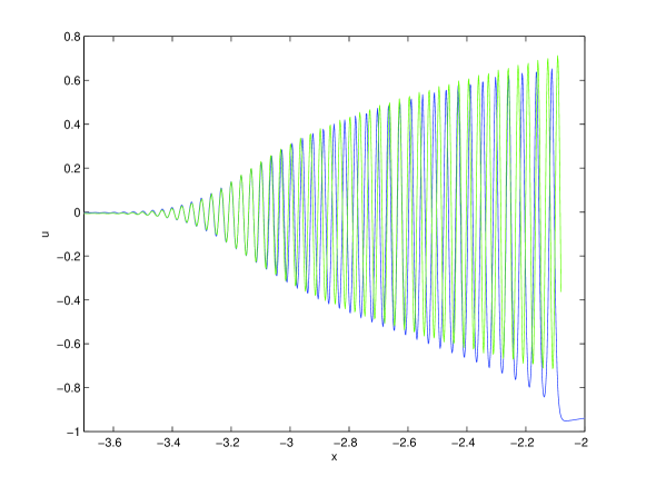
Figure 4. The blue line is the solution of the KdV equation for the initial data $u_{0}(x)=-\mbox{sech}^{2}x$ and $\epsilon=10^{-2}$ for $t=0.4$, and the green line is the corresponding multiscale solution given by formula (3.28).

The difference of the two solutions is shown in Fig. 5.

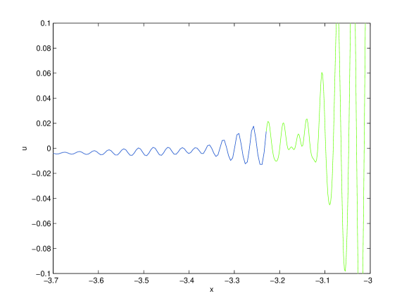
Figure 5. The difference of the KdV and the multiscale solution for the initial data $u_{0}(x)=\mbox{sech}^{2}x$ and $\epsilon=10^{-2}$ for $t=0.4$. The curve is plotted in green in the Whitham zone.

From this figure it is even more obvious that the multiscale solution is a valid approximation in the Whitham zone near the leading edge, but the difference increases rapidly for $|x|\gg x^{-}$.

$\epsilon$ dependence

In [19] it was shown that the asymptotic description becomes more accurate with decreasing $\epsilon$. The same is true for the multiscale solution as can be seen in Fig. 6. The zone, where the multiscale solution gives a better approximation than the asymptotic elliptic solution, shrinks with $\epsilon$. For $x\gg x^{-}(t)$, the multiscale solution is always only a poor approximation to the KdV solution.

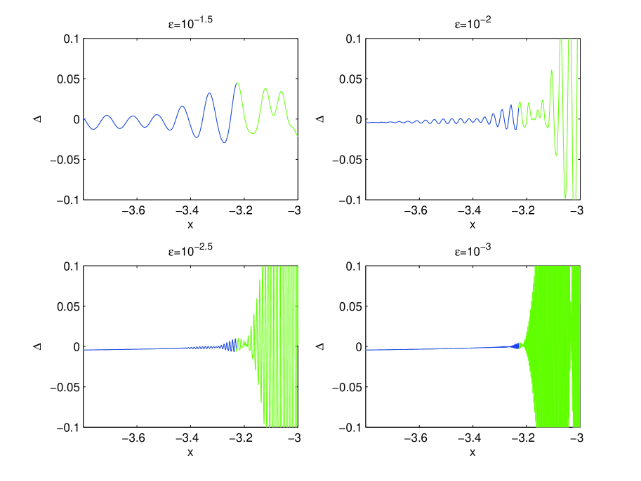
Figure 6. Difference of the KdV and the multiscale solution in order $\epsilon^{1/3}$ for the initial data $u_{0}(x)=-\mbox{sech}^{2}x$ and several values of $\epsilon$ for $t=0.4$. The curves are plotted in green in the Whitham zone.

The maximal difference $\Delta_{max}$ of the KdV solution and the multiscale solution near this edge decreases roughly as $\epsilon^{2/3}$. More precisely the error can be fitted with a straight line by a standard linear regression analysis, $-\log_{10}\Delta_{max}=-a\log_{10}\epsilon+b$ with $a=0.63$, $b=0.41$. The correlation coefficient is $r=0.999$, the standard error is $\sigma_{a}=0.02$.

Comparison and matching with the asymptotic solution

The aim of this paper is to improve the asymptotic description of the small dispersion limit of KdV near the leading edge. In Fig. 7 it can be seen that the multiscale solution will indeed be a much better approximation near this edge.

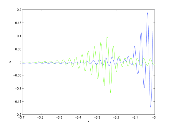
Figure 7. The difference of the KdV and the multiscale solution (blue) and the difference of the KdV and the asymptotic solution (green) for the initial data $u_{0}(x)=-\mbox{sech}^{2}x$ and $\epsilon=10^{-2}$ for $t=0.4$.

Near the leading edge, the multiscale solution provides a superior description of the KdV solution, whereas the elliptic asymptotic solution is much better for $x\gg x^{-}(t)$ in the Whitham zone. In fact it is possible to identify a zone where the multiscale solution is more satisfactory than the asymptotic solution. Due to the strong oscillations of the solutions, there is a certain ambiguity in the definition of this zone. We define the limits of the zone as the last intersection (or where the solutions come closest) on which the other solution has an error with larger oscillations. In this zone it is possible to replace the asymptotic solution by the multiscale solution. The result of this patch work approach is shown in Fig. 8.

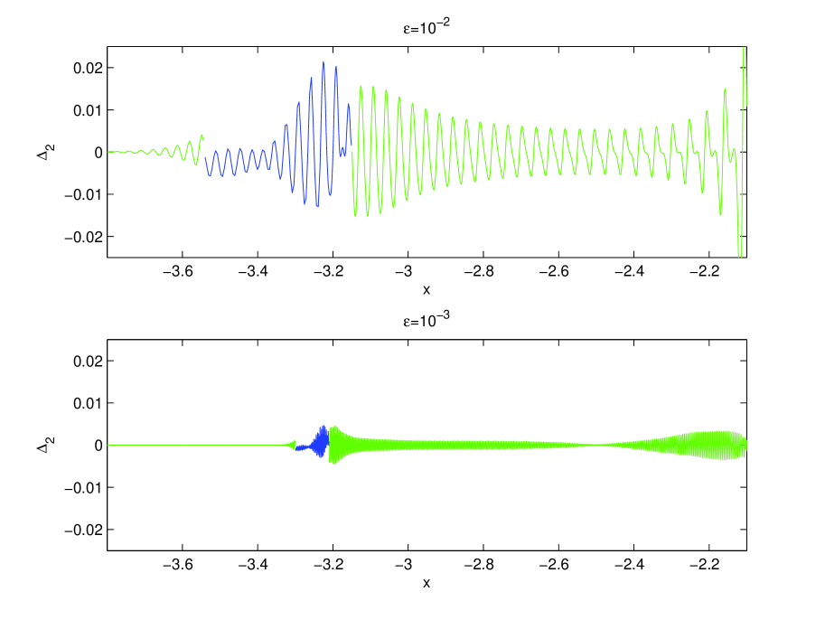
Figure 8. Difference of the KdV and the multiscale solution (blue) and the KdV and the asymptotic solution (green) for the initial data $u_{0}(x)=-\mbox{sech}^{2}x$ at $t=0.4$ for two values of $\epsilon$.

It can be seen that the resulting amended asymptotic description has an accuracy near the leading edge of the same order as in the interior of the Whitham zone. The maximal difference between the KdV and the asymptotic solution still occurs near the leading edge.

As already mentioned, the zone where the multiscale solution provides a better approximation to the KdV solution than the asymptotic solution, shrinks with $\epsilon$ as can be inferred from Fig. 9.

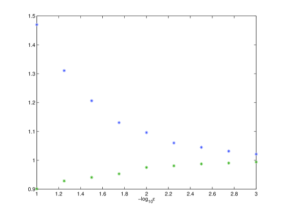
Figure 9. Boundary values of the zone where the multiscale solution provides a better approximation to the KdV solution than the asymptotic solution. The $x$-values of the boundary of this zone (normalized by $x^{-}$) for $t=0.4$ are shown for several values of $\epsilon$.

The width of this zone decreases roughly as $\epsilon^{2/3}$ which shows the self consistency of the used rescaling of the spatial coordinate near the leading edge. More precisely, we find a scaling $\epsilon^{a}$ with $a=0.66$, correlation coefficient $r=0.9996$ and standard error $\sigma_{a}=0.015$. It can be seen that the zone is not symmetric around the leading edge, it extends much further into the Hopf region than in the Whitham zone. This is due to the fact that the multiscale solution is quickly out of phase with the rapid oscillations in the Whitham zone, and that the Hopf solution does not have oscillations.

Breakup time

In [19] it was shown that the elliptic asymptotic solution is worst near the breakup of the Hopf solution. The multiscale expansion obtained in the previous section is not defined for times before $t_{c}$, and it will be worst there, since it can be understood as an expansion around the leading edge of the Whitham zone. At breakup, however, leading and trailing edge coincide. Thus the approximation is rather crude there, but it increases in quality with time as can be seen in Fig. 10. It is, however, interesting to study at which times the multiscale solution starts to give a better asymptotic description than other approaches. Dubrovin conjectured [11] that the asymptotic behavior of the KdV solution close to the breakup of the corresponding Hopf solution is given by a particular solution to the second equation in the Painlevé-I hierarchy. In [20] we provided strong numerical evidence for the validity of this conjecture. The natural question is whether Painlevé-I2 description near the critical point provides a satisfactory asymptotic solution for KdV till times where the the multiscale solution studied in the present paper provides a valid description near the leading edge. A comparison of Fig. 10 with a similar figure in [20] shows that this is qualitatively the case.

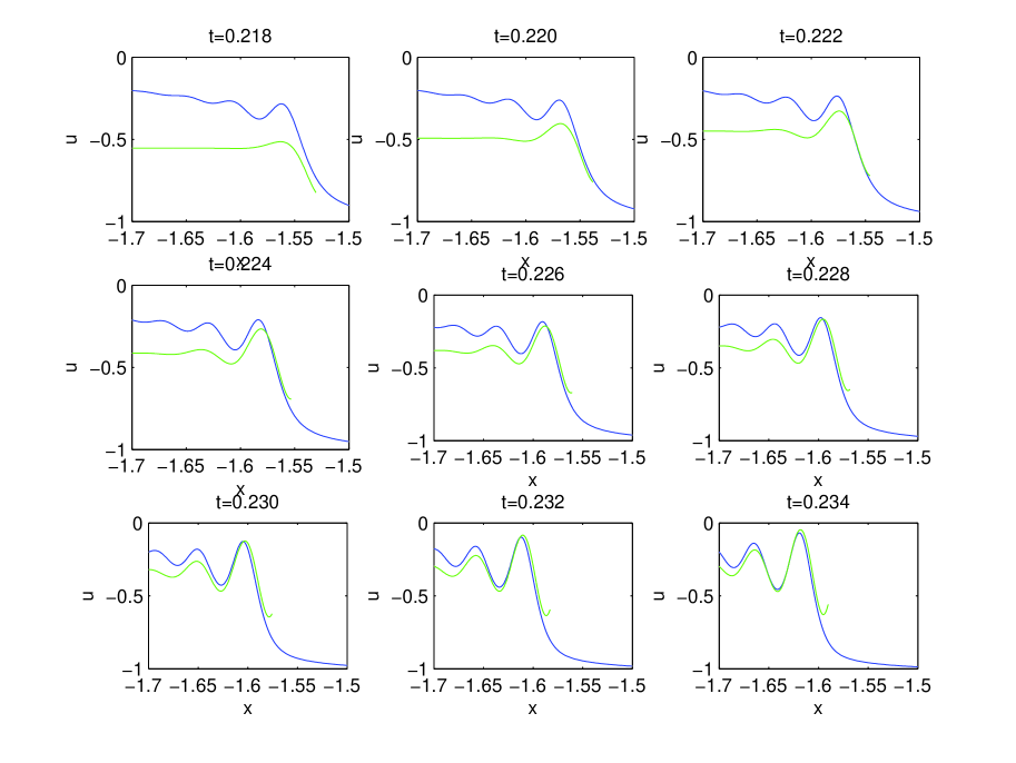
Figure 10. The blue line is the solution of the KdV equation for the initial data $u_{0}(x)=-\mbox{sech}^{2}x$ and $\epsilon=10^{-2}$, and the green line is the corresponding multiscale solution given by formula (3.28). The plots are given for different times near the point of gradient catastrophe $(x_{c},t_{c})$ of the Hopf solution. Here $x_{c}\simeq-1.524$, $t_{c}\simeq 0.216$.

In Fig. 10 the multiscale solution is shown for $x<x^{+}(t)$. Near breakup the approximation is only acceptable close to the breakup point. For larger times, more and more oscillations are satisfactorily reproduced by the multiscale solution. But the multiscale solution will only be a better approximation of the oscillations than the Hopf solution for times $t\gg t_{c}$.

5. Outlook

In the present work we have considered a multiscale solution to the KdV equation in the small dispersion limit close to the leading edge of the oscillatory zone. We studied the solution up to order $\epsilon^{1/3}$ and show that the envelope of the oscillations is described by the Hasting-McLeod solution of the Painlevé-II. The validity of the approach in the considered limit was shown numerically. The double scaling expansion of the KdV solution in the small dispersion limit will be investigated with the Riemann-Hilbert approach and steepest descent method for oscillatory Riemann-Hilbert problem as done in [8]. The Riemann-Hilbert approach seems so far the only analytical tool to study the double-scaling expansion to the Cauchy problem of the KdV equation. This project will be the subject of our future research.

As can be seen from Figure 3, the asymptotic solution of the KdV equation does not give a satisfactory description of the KdV small dispersion limit also at the trailing edge of the oscillatory zone. This problem will be investigated in a subsequent publication, too. A similar problem was tackled in the context of matrix-models in [4].

Appendix A Numerical solution of the Painlevé-II equation

We are interested in the numerical computation of the Hastings-McLeod solution to the Painlevé-II equation

(1.1) $$P_{II}A:=A_{zz}-zA-2A^{3}=0$$

which is subject to the asymptotic conditions [22]

(1.2) $$A\simeq\sqrt{-z/2}\mbox{ for }z\rightarrow-\infty,$$

and

(1.3) $$A\simeq\mbox{Ai}(z)\mbox{ for }z\rightarrow\infty,$$

where $\mbox{Ai}(z)$ is the Airy function. Numerically we will consider equation (1.1) on a finite interval $[z_{l},z_{r}]$ (typically $[-10,10]$). The asymptotic solution near $\pm\infty$, which will be discussed in more detail below, is truncated in a way that the truncation error at $z_{l}$, $z_{r}$ is below $10^{-10}$. At these points we impose the values following from the asymptotic solutions as boundary conditions, namely

$$A(z_{l}) =\sqrt{-z_{l}/2}-\frac{1}{8\sqrt{2}}(-z_{l})^{-5/2}-\frac{73}{128\sqrt{2}}(-z_{l})^{-11/2}$$

(1.4) $$A(z_{r}) =\frac{1}{2\sqrt{\pi}z_{r}^{1/4}}\exp\left(-\frac{2}{3}z_{r}^{3/2}\right).$$

To solve equation (1.1) for $z\in[z_{l},z_{r}]$ we use spectral methods since they allow for an efficient numerical approximation of high accuracy. We map the interval $[z_{l},z_{r}]$ with a linear transformation $z\to x$ to the interval $I=[-1,1]$ and expand $A$ there in Chebychev polynomials.

Let us briefly summarize the Chebychev approach, for details see e.g. [3, 16, 17]. The Chebyshev polynomials $T_{n}(x)$ are defined on the interval $I$ by the relation

$$T_{n}(\cos(t))=\cos(nt)\;,\mbox{where }x=\cos(t)\;,\qquad t\in[0,\pi]\;.$$

A function $f$ on $I$ is approximated via Chebychev polynomials, $f\approx\sum_{n=0}^{N}a_{n}T_{n}(x)$ where the spectral coefficients $a_{n}$ are obtained by the conditions $f(x_{l})=\sum_{n=0}^{N}a_{n}T_{n}(x_{l})$, $l=0,\ldots,N$. This approach is called a collocation method. If the collocation points are chosen to be $x_{l}=\cos(\pi l/N)$, the spectral coefficients follow from $f$ via a Discrete Cosine Transform (DCT) for which fast algorithms exist. We use here a DCT within Matlab. A recursive relation for the derivative of Chebychev polynomials implies that the action of the differential operator $\partial_{x}$ on $f(x)$ leads to an action of a matrix $D$ on the vector of the spectral coefficients $a_{n}$. Thus we express $A(x)$ in terms of Chebychev polynomials, $A(x)=\sum_{n=0}^{N}\tilde{A}_{n}T_{n}(x)$ (we typically work with $N=128$), and the coefficients of $\partial_{x}A$ in terms of Chebychev polynomials are determined then via $D\tilde{A}$.

To solve equation (1.1) on the interval $[z_{l},z_{r}]$, we use an iterative approach,

(1.5) $$A_{n+1,zz}=zA_{n}+2A_{n}^{3},\quad n\in\mathbb{N}.$$

We start with $A_{1}(z)=(1+z^{2})^{1/4}/(1+\exp(z))/\sqrt{2}$. In each step of the iteration we solve equation (1.5) for $A_{n+1}$ with the boundary conditions (1.4). The boundary conditions are imposed with a $\tau$-method: the last two rows of the matrix $D^{2}$ for the second derivative are replaced with the boundary conditions at $x=\pm 1$. Since $T_{n}(\pm 1)=(\pm 1)^{n}$, the resulting matrix $L$ which will be inverted in each step of the iteration, has only $1$ and $-1$ in the last two rows and is thus better conditioned than the matrix $D^{2}$. It turns out that the iteration is unstable if no relaxation is used. We thus define $A_{n+1}=\mu L^{-1}(zA_{n}+2A_{n}^{3})+(1-\mu)A_{n}$ with $\mu=0.009$. With this choice of the parameters, the iteration converges. It is stopped when the difference between $A_{n+1}$ and $A_{n}$ is of the order of machine precision (Matlab works internally with a precision of the order of $10^{-16}$; due to rounding errors machine precision is typically limited to the order of $10^{-14}$). The solution is shown in Fig. 11.

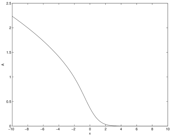
Figure 11. Hastings-McLeod solution of the Painlevé II equation.

To test the accuracy of the solution we plot in Fig. 12 the quantity $P_{II}A$ as computed with spectral methods on the collocation points. It can be seen that the error is biggest on the boundary which is even more obvious from Fig. 13. The found solution is also compared to a numerical solution with a standard ode solver as bvp4c in Matlab. The solutions agree within the limits of numerical precision.

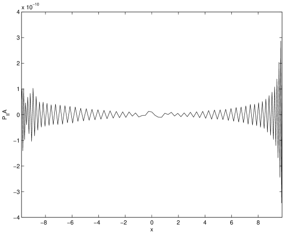
Figure 12. Accuracy of the solution of the Painlevé II equation.

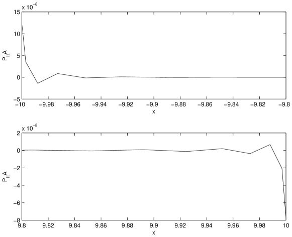
Figure 13. Accuracy of the solution of the Painlevé II equation near the boundary of the considered interval.

For general values of $z$ the solution is obtained as follows: for values of $z\in[z_{l},z_{r}]$ they follow from the spectral data via $A(z)=\sum_{n=0}^{N}\tilde{A}_{n}T_{n}(z)$. Notice that the accuracy of the solution is best on the collocation points, but we can expect it to be of the order of at least $10^{-6}$ even at points $z$ in between. For values of $z<z_{l}$, we use the approximation $A(z)=\sqrt{-z/2}-(-z)^{-5/2}/8/\sqrt{2}-\frac{73}{128\sqrt{2}}(-z_{l})^{-11/2}$, for values of $z>z_{r}$, we use the approximation $A(z)=\exp\left(-\frac{2}{3}z^{3/2}\right)/(2\sqrt{\pi}z^{1/4})$. This provides a global approximation to the solution with an accuracy of the order of $10^{-6}$ and better, which is sufficient for our purposes. Higher precision can be reached within the used approach without problems: one can either increase the values of $-z_{l}$ and $z_{r}$ and use a higher number of polynomials, or use higher order terms in the asymptotic solution of $A$ for $z\to\pm\infty$.

References

• [1] E. Brezin and A. Zee, Universality of the correlations between eigenvalues of large random matrices, Nuclear Physics B 402, 613 627 (1993).
• [2] P.Bleher, A.Its, Double scaling limit in the random matrix model: the Riemann-Hilbert approach. Comm. Pure Appl. Math. 56 (2003), no. 4, 433–516.
• [3] C.Canuto,,M.Y.Hussaini, A.Quarteroni and T.A.Zang, Spectral Methods in Fluid Dynamics, Springer-Verlag, Berlin, 1988.
• [4] T.Claeys, The birth of a cut in unitary random matrix ensembles. Preprint, http://babbage.sissa.it/abs/0711.2609.
• [5] T.Claeys, A.B.J.Kuijlaars, M.Vanlessen, Multi-critical unitary random matrix ensembles and the general Painlevé II equation.To appear in Annals of Mathematics. Preprint http://xxx.lanl.gov/math-ph/0508062.
• [6] P.A. Clarkson, Painlevé equations, nonlinear special functions. Proceedings of the Sixth International Symposium on Orthogonal Polynomials, Special Functions and their Applications (Rome, 2001). J. Comput. Appl. Math. 153 (2003), no. 1-2, 127–140.
• [7] P.A. Clarkson and J.B. McLeod. Arch. Rational Mech. Anal. 103 (1998), pp. 97.
• [8] P.Deift, S.Venakides and X.Zhou, New result in small dispersion KdV by an extension of the steepest descent method for Riemann-Hilbert problems. IMRN 6, (1997), 285-299.
• [9] P.Deift, T.Kriecherbauer, K.R.T.McLaughlin, S.Venakides, X.Zhou, Uniform asymptotics for polynomials orthogonal with respect to varying exponential weights and applications to universality questions in random matrix theory. Comm. Pure Appl. Math. 52 (1999), no. 11, 1335–1425.
• [10] B.Dubrovin, S.P.Novikov, A periodic problem for the Korteweg-de Vries and Sturm-Liouville equations. Their connection with algebraic geometry. Dokl. Akad. Nauk SSSR bf 219, (1974), 531–534.
• [11] B. Dubrovin, On Hamiltonian Perturbations of Hyperbolic Systems of Conservation Laws, II: Universality of Critical Behaviour, Comm. Math. Phys., 267 (2006), 117.
• [12] H.Flaschka, M.Forest, and D.H.McLaughlin, Multiphase averaging and the inverse spectral solution of the Korteweg-de Vries equations. Comm. Pure App. Math. 33 (1980), 739-784.
• [13] A. S. Fokas and A. R. Its, The isomonodromy method and the Painlevé equations, in the book: Important Developments in Soliton Theory, A. S. Fokas, V. E. Zakharov (eds.), Berlin, Heidelb erg, New York, Springer (1993).
• [14] A.S.Fokas, S.Tanveer, A Hele - Shaw problem and the second Painlevé transcendent. Math. Proc. Camb. Phil. Soc. 124 (1998) 169 - 191.
• [15] A.S. Fokas, A.R. Its, and A.V. Kitaev. The isomonodromy approach to matrix models in 2D quantum gravity, Commun. Math. Phys. 147 (1992), 395-430.
• [16] B.Fornberg, A practical guide to pseudospectral methods, (Cambridge University Press, Cambridge 1996)
• [17] J.Frauendiener and C.Klein, Hyperelliptic theta functions and spectral methods. J. Comp. Appl. Math. 167 (2004), no. 1, 193–218.
• [18] Grava, T., Tian, Fei-Ran, The generation, propagation, and extinction of multiphases in the KdV zero-dispersion limit. Comm. Pure Appl. Math. 55 (2002), no. 12, 1569–1639.
• [19] T. Grava and C. Klein, Numerical solution of the small dispersion limit of Korteweg de Vries and Whitham equations, to appear in Comm. Pure Appl. Math. (2007).
• [20] T. Grava and C. Klein, Numerical study of a multiscale expansion of KdV and Camassa-Holm equation, arXiv: math-ph/0702038 (2006).
• [21] A. G.Gurevich, L.P.Pitaevskii, Non stationary structure of a collisionless shock waves. JEPT Letters 17 (1973), 193-195.
• [22] S. P. Hastings and J. B. McLeod, A boundary value problem associated with the second Painlevé transcendent and the Korteweg-de Vries equation. Arch. Rat. Mech. Anal., 73:31D51 (1980).
• [23] A.Its, V.B.Matveev, Hill operators with a finite number of lacunae. (Russian) Funkcional. Anal. i Priložen. 7 (1975), no. 1, 69–70.
• [24] M.C.Jorge, A.A.Minzoni and N.F.Smyth, Modulation solutions for the Benjamin-Ono equation. Phys. D 132 (1999), no. 1-2, 1–18.
• [25] A. A. Kapaev, Global asymptotics of the second Painlevé transcendent. Physics Letters A., 167, 356-362 (1992).
• [26] I.Krichever, The method of averaging for two dimensional integrable equations, Funct. Anal. Appl. 22 (1988), 200-213.
• [27] V.Kudashev, B.Suleimanov, A soft mechanism for the generation of dissipationless shock waves. Physics Letters A 221 (1996), 204-208.
• [28] P. D. Lax and C.D.Levermore, The small dispersion limit of the Korteweg de Vries equation, I,II,III. Comm. Pure Appl. Math. 36 (1983), 253-290, 571-593, 809-830.
• [29] M. Prähofer and H. Spohn, Exact scaling functions for one-dimensional stationary KPZ growth, J. Stat. Phys. 115 (1-2), 255-279 (2004).
• [30] Fei Ran Tian,The initial value problem for the Whitham averaged system. Comm. Math. Phys. 166 (1994), no. 1, 79–115.
• [31] R.S. Rosales. The similarity solution of the Korteweg de Vries equation and the related Painlevé trascendent. Proc. Roy. Soc. London A 361 (1978), pp. 265
• [32] C. A. Tracy and H. Widom, Level spacing distribution and the Airy kernel. Commun. Math. Phys., 159:151 174 (1994).
• [33] S. P.Tsarev, Poisson brackets and one-dimensional Hamiltonian systems of hydrodynamic type. Soviet Math. Dokl. 31 (1985), 488-491.
• [34] S.Venakides, The Korteweg de Vries equations with small dispersion: higher order Lax-Levermore theory. Comm. Pure Appl. Math. 43 (1990), 335-361.
• [35] G. B. Whitham, Linear and nonlinear waves, J.Wiley, New York, 1974.
• [36] www-m5.ma.tum.de/KPZ/