Semi-local string comparison:
Algorithmic techniques and applications
Abstract
A classical measure of string comparison is given by the longest common subsequence (LCS) problem on a pair of strings. We consider its generalisation, called the semi-local LCS problem, which arises naturally in many string-related problems. The semi-local LCS problem asks for the LCS scores for each of the input strings against every substring of the other input string, and for every prefix of each input string against every suffix of the other input string. Such a comparison pattern provides a much more detailed picture of string similarity than a single LCS score; it also arises naturally in many string-related problems. In fact, the semi-local LCS problem turns out to be fundamental for string comparison, providing a powerful and flexible alternative to classical dynamic programming. It is especially useful when the input to a string comparison problem may not be available all at once: for example, comparison of dynamically changing strings; comparison of compressed strings; parallel string comparison. The same approach can also be applied to permutation strings, providing efficient solutions for local versions of the longest increasing subsequence (LIS) problem, and for the problem of computing a maximum clique in a circle graph. Furthermore, the semi-local LCS problem turns out to have surprising connections in a few seemingly unrelated fields, such as computational geometry and algebra of semigroups. This work is devoted to exploring the structure of the semi-local LCS problem, its efficient solutions, and its applications in string comparison and other related areas, including computational molecular biology.
Chapter 1 Introduction
A classical measure of string comparison is given by the longest common subsequence (LCS) problem. Given two strings , of lengths , respectively, the LCS problem asks for the length of the longest possible string that is a subsequence of both and . This length is called the strings’ LCS score. The LCS problem has numerous applications both within and outside computer science. We refer the reader to monographs [61, 90] for the background and further references.
For a more detailed approach to string comparison, let us consider the following generalisation of the LCS problem. Given two strings , as before, the semi-local LCS problem asks for the LCS score of each string against all substrings of the other string, and of all prefixes of each string against all suffixes of the other string. Such a comparison pattern provides a much more detailed picture of string similarity than a single LCS score; it also arises naturally in many string-related problems. Upon closer look, the semi-local LCS problem turns out to be a powerful and flexible alternative to classical dynamic programming in situations where the input to a string comparison problem may not be available all at once: for example, comparison of dynamically changing strings; comparison of compressed strings; parallel string comparison. Furthermore, the semi-local LCS problem turns out to have surprising connections in a few seemingly unrelated fields, such as computational geometry, algebra of semigroups, and graph theory.
This work is devoted to exploring the structure of the semi-local LCS problem, its efficient solutions, and its applications in string comparison and other related areas, including computational molecular biology.
This work is organised as follows. In Chapter 2, we give the necessary preliminaries. In Chapter 3, we investigate the algebraic structure underlying the semi-local LCS problem. This is done in two alternative forms: as matrix distance multiplication on simple unit-Monge matrices, and as a formal monoid of seaweed braids. In Chapter 4, we establish rigorously the relationship between this structure and the semi-local LCS problem. In Chapter 5, we use our structural results to obtain a simple algorithm for the semi-local LCS problem. We also show a number of this algorithm’s applications. In Chapter 6, we generalise our techniques from LCS scores to arbitrary rational-weighted alignment scores and edit distances. In Chapters 7–9, we apply our techniques to several particular classes of string comparison problems: comparison of a periodic string against a plain string; comparison of permutation strings; comparison of compressed strings. In Chapter 10, we explore the connection between semi-local string comparison and a subclass of comparison networks, known as transposition networks. Using this connection, we develop algorithms for several important variants of the LCS problem: parameterised, dynamic, bit-parallel and subword-parallel. In Chapter 11, we discuss ways of extending our techniques beyond semi-local string comparison, towards the ultimate goal of detailed and efficient fully-local string comparison. We also discuss an implementation of our method, which has been used to solve several problems in computational molecular biology.
Chapter 2 Preliminaries
In this chapter, we give the necessary preliminaries for the rest of the work. It is organised as follows. In Section 2.1, we establish the terminology and notation, borrowing main concepts from planar Euclidean geometry and matrix algebra. In Section 2.2, we introduce some basic combinatorial operations on matrices. In Section 2.3, we describe our main algorithmic tool: a special class of integer matrices, called simple unit-Monge matrices. These matrices are intimately related to the combinatorial concept of a permutation, and the dominance counting problem arising in computational geometry.
2.1 Points and matrices
For indices, we will use either integers, or half-integers111The intuition behind using both integers and half-integers is that we are dealing with planar grid-like graphs and, implicitly, with their dual graphs. In this setting, it is natural to index the nodes of a primal graph by pairs of integers, and the nodes of its dual graph (corresponding to the faces of the primal graph) by pairs of half-integers.:
For ease of reading, half-integer variables will be indicated by hats (e.g. , ). Ordinary variable names (e.g. , , with possible subscripts or superscripts), will normally denote integer variables, but can sometimes denote a variable that may be either integer, or half-integer.
It will be convenient to denote
for any integer or half-integer . The set of all half-integers can now be written as
We denote integer and half-integer intervals by
In both cases, the interval is defined by its integer endpoints. For finite intervals and , we call the difference interval length. Note that an integer (respectively, half-integer) interval of length consists of (respectively, ) elements.
To denote infinite intervals of integers and half-integers, we will use and where appropriate. In particular, denotes the set of all integers, and the set of all half-integers.
When dealing with pairs of numbers, we will often use geometric language and call them points. We define two natural strict partial orders on points, called - and -dominance:
| if and | ||||
| if and |
When visualising points, we will deviate from the standard Cartesian convention on the direction of the coordinate axes. We will use instead the matrix indexing convention: the first coordinate in a pair increases downwards, and the second coordinate rightwards. Hence, - and -dominance correspond respectively to the “above-left” and “below-left” partial orders. The latter order corresponds visually to the standard definition of dominance in computational geometry.
We also define the natural lexicographic order on points: point precedes point in this order, if either , or and . The lexicographic order is a strict total order, compatible with the partial -dominance order.
We use standard terminology for special elements and subsets in partial orders. In particular, a set of elements form a chain, if they are pairwise comparable, and an antichain, if they pairwise incomparable. Note that a -chain is a -antichain, and vice versa. An element in a partially ordered set is minimal (respectively, maximal), if, in terms of the partial order, it does not dominate (respectively, is not dominated by) any other element in the set. All minimal (respectively, maximal) elements in a partially ordered set form an antichain.
A function of an integer argument will be called unit-monotone increasing (respectively, decreasing), if for every successive pair of values, the difference between the successor and the predecessor is either or (respectively, or ).
We will make extensive use of vectors and matrices with integer (occasionally, also rational or real) elements, and with integer or half-integer indices222When integers and half-integers are used as matrix indices, it is convenient to imagine that the matrices are written on squared paper. The entries of an integer-indexed matrix are at integer points of line intersections; the entries of a half-integer-indexed matrix are at half-integer points within the squares.. We regard a vector or matrix as a one- (respectively, two-) argument function, so we can speak e.g. about unit-monotone increasing matrices.
Given two index ranges , , it will be convenient to denote their Cartesian product by . We extend this notation to Cartesian products of intervals:
Given index ranges , , a vector over is indexed by , and a matrix over is indexed by , . A vector or matrix is nonnegative, if all its elements are nonnegative.
The matrices we consider can be implicit, i.e. represented by a compact data structure that supports access to every matrix element in a specified (typically small, but not necessarily constant) time. If the query time is not given, it is assumed to be constant by default.
We will use the parenthesis notation for indexing matrices, e.g. . We will also use a straightforward notation for selecting subvectors and submatrices: for example, given a matrix over , we denote by the submatrix defined by the given sub-intervals. A star will indicate that for a particular index, its whole range is being used, e.g. . In particular, and will denote a full matrix column and row, respectively.
We will denote by the transpose of matrix , and by the matrix obtained from by counterclockwise 90-degree rotation. Given a matrix over or , we have
for all .
2.2 Distribution, density and Monge matrices
We now introduce two fundamental combinatorial operations on matrices. The first operation obtains an integer-indexed matrix from a half-integer-indexed matrix by summing up, for each of the integer points, all matrix elements that are -dominated by the given point.
Definition 2.1.
Let be a matrix over . Its distribution matrix over is defined by
for all , . □
The second operation obtains a half-integer-indexed matrix from an integer-indexed matrix, by taking a four-point difference around each given point.
Definition 2.2.
Let be a matrix over . Its density matrix over is defined by
for all , . □
Example 2.3.
We have
■
The definitions of distribution and density matrices extend naturally to matrices over an infinite index range, as long as the sum in Definition 2.1 is defined.
The operations of taking the distribution and the density matrix are close to be mutually inverse. For any finite matrices , as above, and for all , , we have
When matrix is restricted to have all zeros on its bottom-left boundary (i.e. in the leftmost column and the bottom row), the two operations become truly mutually inverse. We introduce special terminology for such matrices.
Definition 2.4.
Matrix over will be called simple, if for all , . Equivalently, is simple if . □
The following classes of matrices play an important role in optimisation theory (see Burkard et al. [39] and Burkard [38] for an extensive survey), and also arise in graph and string algorithms.
Definition 2.5.
Matrix is called totally monotone, if
for all , . □
Definition 2.6.
Matrix is called a Monge matrix, if
for all , . Equivalently, matrix is a Monge matrix, if is nonnegative. Matrix is called an anti-Monge matrix, if is Monge. □
It is easy to see that Monge matrices form a subclass of totally monotone matrices. The characterisation of Monge matrices via their density matrices given by Definition 2.6 is equivalent to the canonical structure theorem for Monge matrices by Burdyuk and Trofimov [37] and Bein and Pathak [23] (see also [39, 38]).
2.3 Permutation and unit-Monge matrices
Our techniques will rely on structures that have permutations as their basic building blocks. We will be dealing with permutations in matrix form, exploiting the symmetry between indices and elements of a permutation.
Definition 2.7.
A permutation333Strictly speaking, such a matrix corresponds to a bijection, rather than a permutation, since the ranges of column and row indices may be different (although they must be of the same cardinality). Therefore, there is a slight abuse of terminology in calling it a permutation matrix, rather than a “bijection matrix”. (respectively, subpermutation) matrix is a zero-one matrix containing exactly one (respectively, at most one) nonzero in every row and every column. □
Example 2.8.
The matrix in Example 2.3 is a permutation matrix. ■
Typically, permutation and subpermutation matrices will be indexed by half-integers.
An identity matrix is a permutation matrix over an interval range , such that , iff . More generally, an offset identity matrix is a permutation matrix over an interval range , where , such that , iff . Note that . Clearly, an identity or offset identity matrix can be represented implicitly in constant space and with constant query time. When dealing with identity and offset identity matrices, we will often omit their index ranges, as long as they are clear from the context.
When dealing with (sub)permutation matrices, we will write “nonzeros” for “index pairs corresponding to nonzeros”, as long as this does not lead to confusion.
Due to the extreme sparsity of (sub)permutation matrices, it would obviously be wasteful and inefficient to store them explicitly. Instead, we will normally assume that a permutation matrix of size is given implicitly by the underlying permutation and its inverse, i.e. by a pair of arrays , , such that for all , and for all . This compact representation has size , and allows constant-time access to each nonzero of by its row index, as well as by its column index. The implicit representation for subpermutation matrices is analogous.
The following subclasses of Monge matrices will play a crucial role in this work.
Definition 2.9.
Matrix is called a unit-Monge (respectively, subunit-Monge) matrix, if is a permutation (respectively, subpermutation) matrix. Matrix is called a unit-anti-Monge (respectively, subunit-anti-Monge) matrix, if is unit-Monge (respectively, subunit-Monge). □
By Definitions 2.6, 2.9, any unit-Monge matrix is subunit-Monge, and any subunit-Monge matrix is Monge (since the corresponding density matrix is a (sub)permutation matrix, and hence nonnegative). Similar inclusions hold for (sub)unit-anti-Monge matrices.
Example 2.10.
The matrix in Example 2.3 is unit-Monge. It is also simple. ■
We will use the following straightforward criterion for a simple integer Monge matrix to be unit-Monge.
Lemma 2.11.
Let be a simple square integer Monge matrix over . Matrix is unit-Monge, if and only if
for all , . □
Proof.
Note that a nonnegative integer matrix over is a permutation matrix, if and only if
for all , . Applying this observation to matrix , we have
| (definition of ) | |||
| (telescoping sum) | |||
| ( simple) | |||
for all . Analogously,
for all . Therefore, is a permutation matrix, so is unit-Monge. ■
The algorithms presented in this work are based on dealing with implicitly represented matrices. While we will occasionally use the term “implicit matrix” in the general sense, it will have the following specific meaning when applied to a (sub)unit-Monge matrix.
Definition 2.12.
Let be a (sub)unit-Monge matrix over . The implicit representation for matrix is given by the (sub)permutation matrix and vectors , :
for all , . □
Our particular focus will be on matrices that are both simple and unit-Monge. Our particular focus will be on square matrices that are both simple and unit-Monge. By Definitions 2.4, 2.9, this holds if and only if , where is a permutation matrix. Definition 2.12 can be specialised to such matrices as follows.
Definition 2.13.
Let be a simple unit-Monge matrix over . The implicit representation for matrix is given by the permutation matrix :
□
Example 2.14.
The matrix in Example 2.3 is simple unit-Monge. ■
Thinking of elements of and as respectively half-integer and integer points in the plane, the value represents the count of nonzeros in , that are -dominated by the point . This type of query to an (implicit) set of points is known as dominance counting. An individual element can be queried in time by a linear sweep of the nonzeros of , counting those that are -dominated by . Using a classical data structure, matrix can be preprocessed to allow element queries on much more efficiently.
Theorem 2.15.
Given a (sub)permutation matrix of size , there exists a data structure that
-
has size ;
-
can be built in time ;
-
allows to query an individual element of the simple (sub)unit-Monge matrix in time ;
□
Proof.
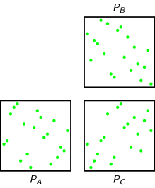
Example 2.16.
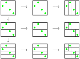
Figure 2.1 shows a permutation matrix, with nonzeros indicated by green444For colour illustrations, the reader is referred to the online version of this work. If the colour version is not available, all references to colour can be ignored. bullets, and the corresponding range tree. ■
The bounds given by Theorem 2.15 can be improved by employing more advanced data structures. Successive improvements to the efficiency of orthogonal range counting (which includes dominance counting as a special case) were obtained by Chazelle [48], JáJá et al. [105], Chan and Pǎtraşcu [44]. The currently most efficient data structure of [44] has size , can be built in time , and answers a dominance counting query in time . However, the standard range tree data structure employed by Theorem 2.15 is simpler, requires a less powerful computation model, and is more likely to be practical. Therefore, we will be using Theorem 2.15 as our main technique for implicit representation of simple (sub)unit-Monge matrices.
In addition to ordinary element queries described by Theorem 2.15, we will also access matrix elements via incremental queries. Given an element of an implicit simple (sub)unit-Monge matrix, such a query returns the value of a specified adjacent element. Incremental queries can be answered directly from the (sub)permutation matrix, without any non-trivial data structures or preprocessing.
Theorem 2.17.
Given a (sub)permutation matrix of size , and the value , , the values , , where they exist, can be queried in time . □
Proof.
Let be a permutation matrix; a generalisation to subpermutation matrices is straightforward. Consider a query of the type ; the proof for other query types is analogous. Let be such that ; value can be obtained from the permutation representation of in time . We have
■
We will call the incremental queries of type columnwise, and of type rowwise. Incremental queries described by Theorem 2.17 can be used to answer batch queries, returning a set of elements in a row, column or diagonal of an implicit simple (sub)unit-Monge matrix. In particular, all elements in a given row, column or diagonal of matrix can be obtained by a sequence of incremental queries in time , and a subset of consecutive elements in time .
Chapter 3 Matrix distance multiplication
In this chapter, we lay the mathematical foundation for the rest of this work. Our main mathematical structure is presented in two alternative forms: first as distance multiplication of simple unit-Monge matrices, and then via an algebraic formalism of seaweed braids. The reader interested primarily in the algorithmic applications of our method may wish to skip this chapter at first reading, and then return to it as necessary for details of specific definitions, theorems and proofs.
This chapter is organised as follows. In Section 3.1, we introduce matrix distance multiplication, and study its algebraic properties in the classes of Monge and simple unit-Monge matrices. In Section 3.2, we describe efficient algorithms for Monge matrices: in particular, row/column minima searching, matrix-vector and matrix-matrix multiplication. In Sections 3.3 and 3.4, we extend these algorithmic results to matrix-vector and matrix-matrix multiplication of simple unit-Monge matrices. In Section 3.5, we define the seaweed braid monoid, and establish its isomorphism with the distance multiplication monoid of simple unit-Monge matrices. In Section 3.6, we describe the first application of our method, obtaining an efficient algorithm for deciding Bruhat comparability of permutations.
3.1 Distance multiplication monoids
The -semiring of integers is one of the fundamental structures in algorithm design. In this semiring, the operators and , denoted by and , play the role of addition and multiplication, respectively. The -semiring is often called distance (or tropical) algebra. For a detailed introduction into this and related topics, see e.g. Rote [153], Gondran and Minoux [88], Butković [40]. An application of the distance algebra to string comparison has been previously suggested by Comet [52].
Throughout this chapter, vectors and matrices will be indexed by integers beginning from , or half-integers beginning from . All our definitions and statements can easily be generalised to indexing over arbitrary integer or half-integer intervals.
Multiplication in the -semiring of integers can be naturally extended to integer matrices and vectors.
Definition 3.1.
Let be a matrix over . Let , be vectors over and respectively. The matrix-vector distance product is defined by
for all . □
Definition 3.2.
Let , , be matrices over , , respectively. The matrix distance product is defined by
for all , . □
We now consider three different monoids of integer matrices with respect to matrix distance multiplication.
Monoid of all nonnegative matrices.
Consider the set of all square matrices with elements in over a fixed index range. This set forms a monoid with zero with respect to distance multiplication. The identity and the zero element in this monoid are respectively the matrices
for all , . For any matrix , we have
Monge monoid.
It is well-known (see e.g. [21]) that the set of all Monge matrices is closed under distance multiplication.
Theorem 3.3.
Let , , be matrices, such that . If , are Monge, then is also Monge. □
Proof.
Let , be over , , respectively. Let , , and , . By definition of matrix distance multiplication, we have
Let , respectively be the values of on which these minima are attained. Suppose . We have
| (definition of ) | |||
| (minimisation over ) | |||
| (term rearrangement) | |||
| ( is Monge) | |||
| (term rearrangement) | |||
| (definition of , ) | |||
The case is treated symmetrically, making use of the Monge property of . Hence, matrix is Monge. ■
Theorem 3.3 implies that the set of all square nonnegative Monge matrices over a fixed index range forms a submonoid (the Monge monoid) in the distance multiplication monoid of all nonnegative matrices (where the range of elements has to be formally extended by ).
The ambient monoid’s identity and zero are inherited by the Monge monoid. Indeed, in the expansion of their density matrices and by Definition 2.2, all indeterminate expressions of the form can be formally considered to be nonnegative. Therefore, matrices and can be formally considered to be Monge matrices.
Unit-Monge monoid.
It is somewhat surprising, but crucial for the development of our techniques, that the set of all simple (sub)unit-Monge matrices is also closed under distance multiplication.
Theorem 3.4.
Let , , be matrices, such that . If , are simple unit-Monge (respectively, simple subunit-Monge), then is also simple unit-Monge (respectively, simple subunit-Monge). □
Proof.
Let , be simple unit-Monge matrices over . We have , , where , are permutation matrices. It is easy to check that matrix is simple, therefore for some matrix .
We now have , and we need to show that is a permutation matrix. Clearly, matrices and are both integer. Furthermore, matrix is Monge by Theorem 3.3, and therefore matrix is nonnegative.
Since is a permutation matrix, we have
for all . Hence
for all , since the minimum is attained respectively at and . Therefore, we have
| (definition of and ) | |||
| (term cancellation) | |||
for all . Symmetrically, we have
for all . Taken together, the above properties imply that matrix is a permutation matrix. Therefore, is a simple unit-Monge matrix.
Finally, let , be simple subunit-Monge matrices over , , respectively. We have , , where , are subpermutation matrices. As before, let , for some matrix ; we have to show that is a subpermutation matrix. Suppose that for some , row contains only zeros. Then, it is easy to check that the corresponding row also contains only zeros, and that upon deleting rows and from the respective matrices, the equality still holds. Symmetrically, a zero column results in a zero column , and upon deleting both these columns from the respective matrices, the equality still holds. Therefore, we may assume without loss generality that , , and that subpermutation matrix (respectively, ) does not have any zero rows (respectively, zero columns).
Let us now extend matrix to a square matrix , where the top rows are filled by zeros and ones so that the resulting matrix is a permutation matrix. Likewise, let us extend matrix to an permutation matrix . We now have
where is an permutation matrix, with matrix occupying its lower-left corner. Hence, matrix is a subpermutation matrix, and the original matrix is a simple subunit-Monge matrix. ■
Theorem 3.4 implies that the set of all simple unit-Monge matrices over a fixed index range forms a submonoid (the unit-Monge monoid) in the Monge monoid.
Without loss of generality, let the matrices be over . The Monge monoid’s identity and zero are neither simple nor unit-Monge matrices, and therefore are not inherited by the unit-Monge monoid. Instead, its identity and zero elements are given respectively by the matrices
(recall that is the matrix obtained by 90-degree rotation of the identity permutation matrix ). For any permutation matrix , we have
Theorem 3.4 gives us the basis for performing distance multiplication of simple (sub)unit-Monge matrices implicitly, by taking the density (sub)permutation matrices as input, and producing a density (sub)permutation matrix as output. It will be convenient to introduce special notation for such implicit distance matrix (and also matrix-vector) multiplication.
Definition 3.5.
Let be a (sub)permutation matrix. Let , be vectors. The implicit matrix-vector distance product is defined by . The implicit matrix-vector distance product is defined analogously. □
Definition 3.6.
Let , , be (sub)permutation matrices. The implicit matrix distance product is defined by . □
The set of all permutation matrices over is therefore a monoid with respect to implicit distance multiplication . This monoid has identity element and zero element , and is isomorphic to the unit-Monge monoid. Note that, although defined on the set of all permutation matrices of size , this monoid is substantially different from the symmetric group , defined by standard permutation composition (equivalently, by standard multiplication of permutation matrices). In particular, the implicit distance multiplication monoid has a zero element , whereas , being a group, cannot have a zero. More generally, the implicit distance multiplication monoid has plenty of idempotent elements (defined by involutive permutations), whereas has the only trivial idempotent . However, both the implicit distance multiplication monoid and the symmetric group still share the same identity element .
3.2 Monge distance multiplication
In this section, we study algorithms for distance multiplication of Monge matrices. For simplicity, we only consider square matrices, although the results generalise to rectangular ones.
We begin with matrix-vector distance multiplication. For generic, explicitly presented matrices, the only reasonable method for matrix-vector distance multiplication of size is by direct application of Definition 3.1 in time .
For implicit Monge matrices (including the case where the matrix is stored in random-access memory, so that only subset of its elements may need to be queried, and the rest can be ignored), the running time can be substantially reduced. This is achieved by an application of a classical row minima searching algorithm by Aggarwal et al. [1] (see also [84]), often nicknamed the “SMAWK algorithm”.
Lemma 3.8 ([1]).
Let be an implicit totally monotone matrix, where each element can be queried in time . The problem of finding the (say, leftmost) minimum element in every row of can be solved in time , where . □
Proof.
Without loss of generality, let be over . Let be an implicit matrix over , obtained by taking every other row of . Clearly, at most columns of contain a leftmost row minimum. The key idea of the algorithm is to eliminate of the remaining columns in an efficient process, based on the total monotonicity property.
We call a matrix element marked (for elimination), if its column has not (yet) been eliminated, but the element is already known not to be a leftmost row minimum. A column gets eliminated when all its elements become marked.
Initially, both the set of eliminated columns and the set of marked elements are empty. In the process of column elimination, marked elements may only be contained in the leftmost uneliminated columns; the value of is initially equal to , and gets either incremented or decremented in every step of the algorithm. The marked elements form a staircase: that is, the marked elements in the first, second, …, -th uneliminated column, are respectively the zero, one, …, topmost elements. In every iteration of the algorithm, two outcomes are possible: either the staircase gets extended to the right to the -st uneliminated column, or the whole -th uneliminated column gets eliminated from matrix , and therefore also from the staircase.
Let , denote respectively the indices of the -th and -st uneliminated column in the original matrix (across both uneliminated and eliminated columns). The outcome of the current iteration depends on the comparison of element , which is the topmost unmarked element in the -th uneliminated column, against element , which is the next uneliminated (and unmarked) element immediately to its right. The outcomes of this comparison and the rest of the elimination procedure are given in Table 3.1.
; ;
while :
case :
case : ;
case : eliminate column
case :
eliminate column
case : ;
case : ;
By storing indices of uneliminated columns in an appropriate dynamic data structure, such as a doubly-linked list, a single iteration of this procedure can be implemented to run in time . The whole procedure runs in time , and eliminates columns.
Let be the matrix obtained from by deleting the eliminated columns. We call the algorithm recursively on . This recursive call returns the leftmost row minima of , and therefore also of . It is now straightforward to fill in the leftmost minima in the remaining rows of in time . Thus, the top level of recursion runs in time . The amount of work gets halved with every recursion level, therefore the overall running time is . ■
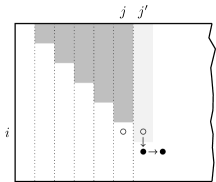
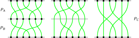
Example 3.9.
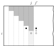
Figure 3.2 gives a snapshot of the two non-boundary cases of the elimination algorithm described in the proof of Lemma 3.8. Each vertical dotted line represents an arbitrary number of consecutive eliminated columns. Dark-shaded cells represent the staircase of marked elements. The current elements , are shown by white circles.
Subfigure 3.2a shows the case , , and Subfigure 3.2b the case , . In both cases, the light-shaded cells represent the newly marked elements. In Subfigure 3.2a, these new elements extend the staircase by one column to the right. In Subfigure 3.2b, the marking of new elements results in the elimination of the whole column , reducing the staircase by its rightmost column. In both cases, the elements , for the next iteration are shown by black circles. ■
It is straightforward to apply the “SMAWK algorithm” of Lemma 3.8 to the distance multiplication of an implicit Monge matrix by a vector.
Theorem 3.10.
Let be an implicit Monge matrix, where each element can be queried in time . Let be an -vector, and an -vector, such that . Given vector , vector can be computed in time , where . □
Proof.
Let for all , . Matrix is an implicit Monge matrix, where each element can be queried in time . The problem of computing the product is equivalent to searching for row minima in matrix , which can be solved in time by Lemma 3.8. ■
The simplest case of application of Theorem 3.10 is when matrix is represented explicitly in random-access memory. In such case, we have , and Monge matrix-vector multiplication can be performed in time , without even reading most elements of the matrix.
We now consider matrix-matrix distance multiplication. For generic, explicitly presented matrices, direct application of Definition 3.2 gives an algorithm for matrix distance multiplication of size , running in time . Slightly subcubic algorithms for this problem have also been obtained. The fastest currently known algorithm is by Chan [45], running in time .
For Monge matrices, distance multiplication can easily be performed in quadratic time (see also [21]). For simplicity, we restrict ourselves to square Monge matrices.
Theorem 3.11.
Let , , be matrices, such that is Monge, and . Given matrices , , matrix can be computed in time and memory . □
Proof.
The problem of computing the product is equivalent to instances of the matrix-vector product , where (respectively, ) is a column of (respectively, ). Every one of these instances can be solved in time by Theorem 3.10, so the overall running time is .
Alternatively, an algorithm with the same asymptotic running time can be obtained directly by the divide-and-conquer technique (see e.g. [15]). ■
3.3 Unit-Monge matrix-vector distance multiplication
We will now discuss algorithms for multiplication of implicit simple unit-Monge matrices. We begin with matrix-vector multiplication, which turns out to be already a non-trivial problem.
By Theorem 2.15, an element of an implicit simple unit-Monge matrix, represented by an appropriate data structure, can be queried in time . By plugging this query time into Theorem 3.10, we obtain immediately an algorithm for implicit matrix-vector distance multiplication, running in time .
A more careful analysis of the elimination procedure of Lemma 3.8 shows that the required matrix elements can be obtained, instead of the standalone element queries of Theorem 2.15, by more efficient incremental queries of Theorem 2.17. At the top level of recursion, the query time is . However, the query time per matrix element grows with each recursion level, as the queried elements become more and more distant from each other with respect to the original top-level matrix. The resulting combined query time is in every recursion level, so the overall running time becomes .
We now show that it is possible to speed up the implicit matrix-vector distance multiplication algorithm still further. We describe two solutions: first, a relatively straightforward extension of the elimination procedure of Lemma 3.8, running in time ; second, an algorithm based on sophisticated data structures for the union-find problem in the unit-cost RAM model, running in optimal time .
The first solution, using incremental queries and a new “coarse-grain” recursive fill-in procedure, is as follows.
Lemma 3.12.
Let be an implicit (sub)unit-Monge matrix over , represented as in Definition 2.12 by the (sub)permutation matrix and vectors , . The problem of finding the (say, leftmost) minimum element in every row of can be solved in time , where . □
Proof.
First, observe that vector has no effect on the positions (as opposed to the values) of any row minima. Therefore, we assume without loss of generality that for all (and, in particular, ). Further, suppose that some column is identically zero; then, depending on whether or , we may delete respectively column or as it does not contain any leftmost row minima. Also, suppose that some row is identically zero; then the minimum value in row lies in the same column as the minimum value in row , hence we can delete one of these rows. Therefore, we assume without loss of generality that is an implicit unit-Monge matrix over , and hence is a permutation matrix.
To find the leftmost row minima, we adopt the column elimination procedure of Lemma 3.8 (see Table 3.1, Figure 3.2), with some modifications outlined below.
Let be an implicit matrix, obtained by taking a subset of rows of at regular intervals of . Clearly, at most columns of contain a leftmost row minimum. We need to eliminate of the remaining columns.
Let be over . Throughout the elimination procedure, we maintain a vector , , initialised by zero values. In every iteration, given a current value of the index , each value gives the count of nonzeros within the rectangle , .
Consider an iteration of the column elimination procedure of Lemma 3.8 with given values , , , operating on matrix elements , . For the iteration that follows the current one, the following matrix elements may be required:
-
, . These values can be obtained respectively as and .
-
, . These values can be obtained respectively from , by a rowwise incremental query of matrix via Theorem 2.17, plus a single access to vector .
-
. This element was already queried in the iteration at which its column was first added to the staircase. There is at most one such element per column, therefore each of them can be stored and subsequently queried in constant time.
At the end of the current iteration, index may be incremented (i.e. the staircase may grow by one column). In this case, we also need to update vector for the next iteration. Let be such that . Let ; we have . The update consists in incrementing the vector element by .
The total number of iterations in the elimination procedure is at most . This is because in total, at most columns are added to the staircase, and at most (in fact, exactly ) columns are eliminated. Therefore, the elimination procedure runs in time .
Let be the matrix obtained from by deleting the eliminated columns. Using incremental queries to matrix , it is straightforward to obtain matrix explicitly in random-access memory in time . We now call the algorithm of Lemma 3.8 to compute the row minima of , and therefore also of , in time .
We now need to fill in the remaining row minima of matrix . The row minima of matrix define a chain of submatrices in at which these remaining row minima may be located. More specifically, given two successive row minima of , all the row minima that are located between the two corresponding rows in must also be located between the two corresponding columns. Each of the resulting submatrices has rows; the number of columns may vary from submatrix to submatrix. It is straightforward to eliminate from each submatrix all columns not containing any nonzero of matrix ; therefore, without loss of generality, we may assume that every submatrix is of size .
We now call the algorithm recursively on each submatrix to fill in the remaining leftmost row minima. The amount of work remains in every recursion level. There are recursion levels, therefore the overall running time of the algorithm is . ■
Example 3.13.
A faster, time-optimal solution was suggested by Gawrychowski [82].
Lemma 3.14.
Under the conditions of Lemma 3.12, the running time can be reduced to . □
Proof.
As before, observe that vector has no effect on the positions of any row minima. Therefore, we assume without loss of generality that for all , so for all , . Also note that we can perturb the elements of vector slightly, so that each leftmost row minimum becomes the only minimum in its row. Therefore, from now on we will omit the adjective “leftmost”.
Consider vector , which coincides with the bottom row of matrix : . Suppose that for some , , , we have . Then, the element cannot be the minimum in row . Furhermore, by the Monge property of matrix , we have for all , therefore an element cannot be the minimum in any row , and hence column can be safely excluded from the search for row minima. After excluding all such columns, the remaining elements in row form a decreasing subsequence of record minimal values, which we call for short the record subsequence. Here, an element is called a record minimal value, if we have for all . The record subsequence can be found trivially in a single pass of the input vector in time . The final element in the record subsequence is the row minimum in row .
Let be the indices of the record minimal values in row , so the initial record subsequence is
Our goal now is to compute the record subsequence for every row in matrix . We will represent the record subsequences implicitly by storing the differences between successive pairs of elements. In particular, the initial record subsequence is represented by the sequence of (all negative) values
We now move through rows of matrix from the bottom row towards the top row , updating the implicit record subsequence incrementally for each row. We describe the procedure for updating this subsequence from row to row ; the other updates are analogous.
Let be the nonzero of matrix in row . Let
Recall that for all , . Assuming that both and above are well-defined (i.e. the set under respectively the and the operator is non-empty), it is easy to see that the record subsequence in row is
In other words, we take all the elements of the record subsequence from to inclusive, we delete all the elements strictly between and , and then we take all the elements from to , incrementing them by .
The described updated record subsequence is represented implicitly by the updated difference sequence
In other words, we take all the elements of the original difference subsequence from to inclusive, we delete all the elements from to inclusive, we create a new element , and then we take all the elements of the original difference subsequence from to inclusive. Assuming indices and are known, such an update can be performed in time .
In case is undefined (this happens whenever ), the updated record subsequence becomes
hence the corresponding difference sequence remains the same as for the original record subsequence, and does not need to be updated. In case is undefined (this happens whenever ), the record subsequence becomes
hence the corresponding difference sequence is obtained by taking the original record subsequence from to inclusive. In both above cases, the update can still be performed in time .
Now, assume that only index is known before the start of the update. Then, index can be found by linear search through the difference sequence. The size of this linear search is equal to the number of elements deleted from the sequence by the subsequent update. Hence, the amortized running time of the linear search across all the updates is .
It remains to show how to find the index efficiently. Consider the partitioning of interval into a disjoint union of sub-intervals
The problem of finding is equivalent to finding the interval containing the index of the nonzero . The same problem has to be solved repeatedly for each subsequent row, where we need to find the interval between elements of the current record subsequence, containing the current nonzero of matrix . As elements get deleted from the record subsequence by the update, pairs of adjacent intervals also have to be merged into one interval.
The described problem fits in the classical setup of the union-find problem, in particular its special case called the interval union-find problem (see e.g. Italiano and Raman [103]). This is a highly non-trivial problem that, in the most general setting, has a marginally superlinear lower bound on the running time. However, in the unit-cost RAM model of computation this problem can be solved by an algorithm of Gabow and Tarjan [80] (see also [103]) in time .
The overall running time of the algorithm (assuming, as usual, the unit-cost RAM model of computation) is . ■
Lemma 3.14 can now be applied to obtain an optimal algorithm for distance multiplication of a simple (sub)unit-Monge matrix by a vector.
Theorem 3.15.
Let be an (sub)permutation matrix. Let be an -vector, and an -vector, such that . Given the nonzeros of and the full vector , vector can be computed in time , where . □
3.4 Unit-Monge matrix-matrix distance multiplication
We now consider matrix-matrix distance multiplication. While the quadratic running time of Theorem 3.11 is trivially optimal for explicit matrices, it is possible to break through this time barrier in the case of implicitly represented matrices.
For simplicity, we restrict ourselves once again to square matrices (which is trivially the case for unit-Monge matrices, but not so for subunit-Monge matrices). Subquadratic distance multiplication algorithms for implicit simple (sub)unit-Monge matrices were given in [163, 166], and culminated with the following result in [169].
Theorem 3.16.
Let , , be (sub)permutation matrices, such that . Given the nonzeros of , , the nonzeros of can be computed in time . □
Proof.
Let , , be permutation matrices over . The algorithm follows a divide-and-conquer approach, in the form of recursion on .
-
Recursion base: .
The computation is trivial.
-
Recursive step: .
Assume without loss of generality that is even. Informally, the idea is to split the range of index in the definition of matrix distance product (Definition 3.2) into two sub-intervals of size . For each of these half-sized sub-intervals of , we use the sparsity of the input permutation matrix (respectively, ) to reduce the range of index (respectively, ) to a (not necessarily contiguous) subset of size ; this completes the divide phase. We then call the algorithm recursively on the two resulting half-sized subproblems. Using the subproblem solutions, we reconstruct the output permutation matrix ; this is the conquer phase.
We now describe each phase of the recursive step in more detail.
-
Divide phase.
By Definition 3.6, we have
Consider the partitioning of matrices , into subpermutation matrices
where , , , are over , , , , respectively; in each of these matrices, we maintain the indexing of the original matrices , . We now have two implicit matrix multiplication subproblems
where , are of size . Each of the subpermutation matrices , , , , , has exactly nonzeros.
Recall from the proof of Theorem 3.4 that a zero row in (respectively, a zero column in ) corresponds to a zero row (respectively, column) in their implicit distance product . Therefore, we can delete all zero rows and columns from , , , obtaining, after appropriate index remapping, three permutation matrices. Consequently, the first subproblem can be solved by first performing a linear-time index remapping (corresponding to the deletion of zero rows and columns from , ), then making a recursive call on the resulting half-sized problem, and then performing an inverse index remapping (corresponding to the reinsertion of the zero rows and columns into ). The second subproblem can be solved analogously.
-
Conquer phase.
We now need to combine the solutions for the two subproblems to a solution for the original problem. Note that we cannot simply put together the nonzeros of the subproblem solutions. The original problem depends on the subproblems in a more subtle way: some elements of depend on elements of both and , and therefore would not be accounted for directly by the solution to either subproblem on its own. A similar observation holds for elements of . However, note that the nonzeros in the two subproblems have disjoint index ranges, and therefore the direct combination of subproblem solutions , although not a solution to the original problem, is still a permutation matrix.
In order to combine correctly the solutions of the two subproblems, let us consider the relationship between these subproblems in more detail. First, we split the range of index in the definition of matrix distance product (Definition 3.2) into a “low” and a “high” sub-interval, each of size .
(3.1) for all . Let us denote the two arguments in (3.1) by and , respectively:
(3.2) for all . The first argument in (3.1), (3.2) can be expressed via the solutions of the two subproblems as follows:
(definition of ) (term rearrangement) (definition of ) (3.3) Here, the final equality is due to
since the minimum is attained at . The second argument in (3.1), (3.2) can be expressed analogously as
(3.4) The minimisation operator in (3.1), (3.2) is equivalent to evaluating the sign of the difference of its two arguments:
(by (3.3), (3.4)) (term rearrangement) (definition of ) (definition of , ) Since , are subpermutation matrices, and a permutation matrix, it follows that function is unit-monotone increasing in each of its arguments.
The sign of function determines the positions of nonzeros in as follows. Let us fix some half-integer point in , and consider the signs of the four values at neighbouring integer points. Due to the unit-monotonicity of , only three cases are possible.
-
Case for all four sign combinations. We have
for each sign combination taken consistently on both sides of the inequality, and, by (3.2),
Hence, we have
(definition of , , (3.3), (3.4)) Thus, in this case is equivalent to . Note that this also implies , since otherwise we would have for all four sign combinations, and hence, by symmetry, also . However, that would imply , which is a contradiction to being a permutation matrix.
-
Case for all four sign combinations. Symmetrically to the previous case, we have
Thus, in this case is equivalent to , and implies .
Summarising the above three cases, we have , if and only if one of the following conditions holds:
and (3.5) and (3.6) and (3.7) By the discussion above, these three conditions are mutually exclusive.
In order to check the conditions (3.5)–(3.7), we need an efficient procedure for determining the sign of function in points of the integer square . Informally, low (respectively, high) values of both and correspond to negative (respectively, positive) values of . By unit-monotonicity of , there must exist a pair of monotone rectilinear paths from the bottom-left to the top-right corner of the half-integer square , that separate strictly negative and nonnegative (respectively, strictly positive and nonpositive) values of .
We now give a simple efficient procedure for finding such a pair of separating paths. By symmetry we only need to the consider the lower separating path. For all integer points above-left (respectively, below-right) of this path, we have (respectively, ).
We start at the bottom-left corner of the square, with as the initial point on the lower separating path. We have .
Let now denote any current point on the lower separating path, and suppose that we have evaluated . The sign of this value determines the next point on the path:
if if Following this choice, we then evaluate either , or from by an incremental query of Theorem 2.17 in time . The computation is now repeated with the new current point.
The described path-finding procedure runs until either , or . We then complete the path by moving in a straight horizontal (respectively, vertical) line to the final destination . The whole procedure of finding the lower separating path runs in time . A symmetric procedure procedure with the same running time can be used to find the upper separating path, for which we have on the above-left, and on the below-right.
Given a value , let us now consider the set of points with ; such a set forms a diagonal in the half-integer square. Let , where , be the unique intersection point of the given diagonal with the lower separating path. Let . Define analogously, using the upper separating path. Conditions (3.5)–(3.7) can now be expressed in terms of arrays , as follows:
and (3.8) and (3.9) (3.10) Here, we make use of the fact that is equivalent to , and to .
The nonzeros of satisfying either of the conditions (3.8), (3.9) can be found in time by checking directly each of the nonzeros in matrices and . The nonzeros of satisfying condition (3.10) can be found in time by a linear sweep of the points on the two separating paths. We have now obtained all the nonzeros of matrix .
-
- (End of recursive step)
The generalisation to subpermutation matrices is as in Theorem 3.4.
-
Time analysis.
The recursion tree is a balanced binary tree of height . In the root node, the computation runs in time . In each subsequent level, the number of nodes doubles, and the running time per node decreases by a factor of . Therefore, the overall running time is .
■
Example 3.17.
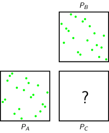
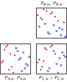
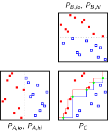
Figure 3.3 illustrates the proof of Theorem 3.16 on a problem instance with a solution generated by the Wolfram Mathematica software. Subfigure 3.3a shows a pair of input permutation matrices , , with nonzeros indicated by green circles. Subfigure 3.3b shows the partitioning of the implicit matrix distance multiplication problem into two subproblems. The nonzeros in the two subproblems are shown respectively by filled red squares and hollow blue squares. Subfigure 3.3c shows a recursive step. The lower and the upper separating paths are shown respectively in red and in blue (note that the lower path is visually above the upper one; the lower/upper terminology refers to the relative values of , rather than the visual position of the paths). The nonzeros in the output matrix satisfying (3.8), (3.9), (3.10) are shown respectively by filled red squares, hollow blue squares, and green circles; note that overall, there are 20 such nonzeros, and that they define a permutation matrix. Subfigure 3.3d shows the output matrix . ■
3.5 Seaweed braids
Further understanding of the unit-Monge monoid (and, by isomorphism, of the implicit distance multiplication monoid of permutation matrices) can be gained via an algebraic formalism closely related to braid theory. We refer the reader to [110] for the background on classical braid theory.
Consider two sets of nodes each, drawn on two parallel horizontal lines in the Euclidean plane. We put the two node sets into one-to-one correspondence by connecting them pairwise, in some order, with continuous monotone curves. (Here, a curve is called monotone, if its vertical projection is always directed downwards.) These curves will be called seaweeds111A tongue-in-cheek justification for this term is that seaweed braids are like ordinary braids, except that they are sticky: a pair of seaweeds, once they have crossed, cannot be fully untangled.. We call the resulting configuration a seaweed braid of width .
There is remarkable similarity between seaweed braids and classical braids. However, there is also a crucial difference: all crossings between seaweeds are “level crossings”, i.e. a pair of crossing seaweeds are not assumed to pass under/over one another as in classical braids. We will also assume that all crossings are between exactly two seaweeds, hence three or more seaweeds can never meet at a single point.
In a seaweed braid, a given pair of seaweeds may cross an arbitrary number of times. We call a seaweed braid reduced, if every pair of its seaweeds cross at most once (i.e. either once, or not at all).
Similarly to classical braids, two seaweed braids of the same width can be multiplied. The product braid is obtained as follows. First, we draw one braid above the other, identifying the bottom nodes of the top braid with the top nodes of the bottom braid. Then, we join up each pair of seaweeds that became incident in the previous step. Note that, even if both original seaweed braids were reduced, their product may in general not be reduced.
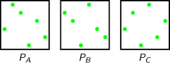
Example 3.19.
In Subfigure 3.1b, the left-hand side is a product of two reduced seaweed braids. In this product braid, some pairs of seaweeds cross twice, hence it is not reduced. ■
Seaweed braids can be transformed (and, in particular, unreduced braids can be reduced) according to a specific set of algebraic rules. These rules are incorporated into the following formal definition.
Definition 3.20.
The seaweed monoid is a finitely presented monoid on generators: (the identity element), , , …, . The presentation of monoid consists of the idempotence relations
| (3.11) | ||||||
| the far commutativity relations | ||||||
| (3.12) | ||||||
| and the braid relations | ||||||
| (3.13) | ||||||
□
Traditionally, this structure is also known as the -Hecke monoid of the symmetric group , or the Richardson–Springer monoid (for details, see e.g. Denton et al. [66], Mazorchuk and Steinberg [134], Deng et al. [65]).


The correspondence between elements of the seaweed monoid and seaweed braids is as follows. The monoid multiplication (i.e. concatenation of words in the generators) corresponds to the multiplication of seaweed braids. The identity element corresponds to a seaweed braid where the top nodes are connected to the bottom nodes in the left-to-right order, without any crossings. Each of the remaining generators corresponds to an elementary crossing, i.e. to a seaweed braid where the only crossing is between a pair of neighbouring seaweeds in half-integer positions and . Figure 3.4 shows the defining relations of the seaweed monoid (3.11)–(3.13) in terms of seaweed braids.
Example 3.21.
In Subfigure 3.1b, the left-hand side is an unreduced product of two seaweed braids. We now comb the seaweeds by running through all their crossings, respecting the top-to-bottom partial order of the crossings. For each crossing, we check whether the two crossing seaweeds have previously crossed above the current point. If this is the case, then we undo the current crossing by removing it from the braid and replacing it by two non-crossing seaweed pieces. The correctness of this combing procedure is easy to prove by the seaweed monoid relations (3.11)–(3.13). After all the crossings have been combed, we obtain a reduced seaweed braid shown in the middle of Subfigure 3.1b. Another equivalent reduced seaweed braid in shown in the right-hand side. ■
A permutation matrix over can be represented by a seaweed braid as follows. The row and column indices correspond respectively to the top and the bottom nodes, ordered from left to right. A nonzero corresponds to a seaweed connecting top node and bottom node . For a given permutation, it is always possible to draw the seaweeds so that the resulting seaweed braid is reduced. In general, this reduced braid will not be unique; however, it turns out that all the reduced braids corresponding to the same permutation are equivalent. We formalise this observation by the following lemma.
Lemma 3.22.
The seaweed monoid consists of at most distinct elements. □
Proof.
It is straightforward to see that any seaweed braid can be transformed into a reduced one, using relations (3.11)–(3.13). Then, any two reduced seaweed braids corresponding to the same permutation can be transformed into one another, using far commutativity (3.12) and the braid relations (3.13). Therefore, each permutation corresponds to a single element of . This mapping is surjective, therefore the number of elements in is at most the total number of permutations . ■
We now establish a direct connection between elements of the seaweed monoid and permutation matrices. The identity generator corresponds to the identity matrix . Each of the remaining generators corresponds to an elementary transposition matrix , defined as
Lemma 3.23.
The set , , generates the full distance multiplication monoid of simple unit-Monge matrices. □
Proof.
Let be a permutation matrix. Consider an arbitrary reduced seaweed braid corresponding to , and let be the position of its first elementary crossing. Consider the truncated seaweed braid, obtained by removing this seaweed crossing. This braid is still reduced, and such that the pair of seaweeds originating in , do not cross. Let this pair of seaweeds terminate at indices , , where . Let be the permutation matrix corresponding to the truncated seaweed braid. We have
We will now show that or, equivalently . The lemma statement then follows by induction.
Note that and for all , , and for all . Therefore, we have
for all , , and for all .
It remains to consider the case . Note that for all , . Let . We have
| (3.14) |
By definition of the distribution matrix (Definition 2.1), we have
Hence, we have
and, analogously,
We have established that the value under the minimum operator in (3.14) for is always no less than the values for both and . Therefore, the minimum is never attained solely at , so we may assume . We now consider two cases: either , or .
For , we have . Therefore,
| (attained at ) | |||
Similarly, for , we have . Therefore,
| (attained at ) | |||
Substituting into (3.14), we now have
Recall that . We have
| for | ||||
| for | ||||
| for |
In all three above cases, we have
which completes the proof. ■
We are now able to establish a formal connection between the unit-Monge monoid and the seaweed monoid.
Theorem 3.24.
The distance multiplication monoid of simple unit-Monge matrices is isomorphic to the seaweed monoid . □
Proof.
We have already established a bijection between the generators of both monoids: a generator simple unit-Monge matrix corresponds to a generator of the seaweed monoid . It is straightforward to check that relations (3.11)–(3.13) are verified by matrices , therefore the bijection on the generators defines a homomorphism from the seaweed monoid to the unit-Monge matrix monoid. By Lemma 3.23, this homomorphism is surjective, hence the cardinality of is at least the number of all simple unit-Monge matrices of size , equal to . However, by Lemma 3.22, the cardinality of is at most . Thus, the cardinality of is exactly , and the two monoids are isomorphic. ■
Example 3.25.
The seaweed monoid is closely related to some other well-known algebraic structures:
A generalisation of the seaweed monoid is given by -Hecke monoids of general Coxeter groups, also known as Coxeter monoids. These monoids arise naturally as subgroup monoids in groups. The theory of Coxeter monoids can be traced back to Bourbaki [34], and was developed in [172, 150, 78, 35]. A further generalisation to -trivial monoids has been studied by Denton et al. [66]. The contents of this chapter can be regarded as a first step in the algorithmic study of such general classes of monoids.
3.6 Bruhat order
Given a permutation, it is natural to ask how well-sorted it is. In particular, a permutation may be either fully sorted (the identity permutation), or fully anti-sorted (the reverse identity permutation), or anything in between. More generally, given two permutations, it is natural to ask whether, in some sense, one is “more sorted” than the other.
Let , be permutation matrices over . A classical “degree-of-sortedness” comparison is given by the following partial order (see e.g. Bóna [33], Hammett and Pittel [92], and references therein).
Definition 3.26.
Matrix is lower than matrix in the Bruhat order, , if can be transformed to by a sequence of anti-sorting steps. Each such step substitutes a (not necessarily contiguous) submatrix of the form by a submatrix of the form . □
Informally, , if defines a “more sorted” permutation than . More precisely, , if the permutation defined by can be transformed into the one defined by by successive pairwise anti-sorting between arbitrary pairs of elements. Symmetrically, the permutation defined by can be transformed into the one defined by by successive pairwise sorting (or, equivalently, by an application of a comparison network; see e.g. Knuth [116]).
Bruhat order is an important group-theoretic concept, which can be generalised to arbitrary Coxeter groups (see Björner and Brenti [32], Denton et al. [66] for more details and further references).
Many equivalent definitions of the Bruhat order on permutations are known; see e.g. Björner and Brenti [32], Drake et al. [70], Johnson and Nasserasr [106]. Probably the simplest one, known as Ehresmann’s tableau criterion [92] or dot criterion [32], is as follows.
Theorem 3.27.
We have , if and only if elementwise. □
Proof.
Straightforward from the definitions; see [32]. ■
Example 3.28.
We have
Note that the permutation matrix on the right can be obtained from the one on the left by anti-sorting the submatrix at the intersection of the top two rows with the leftmost and rightmost columns.
We also have
The above two permutation matrices are incomparable in the Bruhat order. ■
Theorem 3.27 immediately gives one an algorithm for deciding whether two permutations are Bruhat-comparable in time . To the author’s knowledge, no asymptotically faster algorithm for deciding Bruhat comparability has been known so far.
To demonstrate an application of our techniques, we now give a new characterisation of the Bruhat order in terms of the unit-Monge monoid (or, equivalently, the seaweed monoid). This characterisation will give us a substantially faster algorithm for deciding Bruhat comparability.
Intuitively, the connection between the Bruhat order and seaweeds is as follows. Consider matrix and the rotated matrix . The matrix rotation induces a one-to-one correspondence between the nonzeros of and , and therefore also between individual seaweeds in their reduced seaweed braids. A pair of seaweeds cross in a reduced braid of , if and only if the corresponding pair of seaweeds do not cross in a reduced braid of . Now consider the product braid , where each seaweed is made up of two mutually corresponding seaweeds from and , respectively. Every pair of seaweeds in braid either cross in the top sub-braid , or in the bottom sub-braid , but not in both. Therefore, the product braid is a reduced seaweed braid, in which every pair of seaweeds cross exactly once. Thus, we have .
Now suppose . By Theorem 3.27, we have elementwise. Therefore, by Definition 3.2, elementwise, hence by Theorem 3.27, we have . However, as argued above, , which is the highest possible permutation matrix in the Bruhat order, corresponding to the reverse identity permutation. Therefore, . We thus have a necessary condition for . It turns out that this condition is also sufficient, giving us a new, computationally efficient criterion for Bruhat comparability.
Theorem 3.29.
We have , if and only if . □
Proof.
Let . We have
| (definition of ) | |||
| (term rearrangement) | |||
| (3.15) |
We now prove the implication separately in each direction.
- Necessity.
- Sufficiency.
■
The combination of Theorems 3.16 and 3.29 gives us a fast algorithm for deciding Bruhat comparability of permutations.
Theorem 3.30.
Given permutation matrices , , it is possible to determine whether in time . □
Chapter 4 Semi-local string comparison
In this chapter, we introduce semi-local string comparison, and establish its connection with the mathematical concepts of the previous chapter.
This chapter is organised as follows. In Sections 4.1, 4.2, we formally define the LCS and the semi-local LCS problems. In Section 4.3, we describe a representation of the semi-local LCS problem by an alignment dag, and introduce the associated score matrix and seaweed matrix. In Section 4.4, we introduce some further notation relevant to the semi-local LCS problem. In Section 4.5, we discuss the fundamental operation of seaweed matrix composition. We then obtain an efficient algorithm for this operation, based on the algebraic framework developed in the previous chapter.
4.1 The LCS problem
We will consider strings of characters taken from an alphabet. No a priori assumptions are made on the size of the alphabet and on the set of primitive character operations; we will make specific assumptions in different contexts (e.g. a fixed finite alphabet with only equality comparisons, or an alphabet of integers up to a given with standard arithmetic operations, etc.) Two alphabet characters , match, if , and mismatch otherwise. In addition to alphabet characters, we introduce two special extra characters: the guard character ‘$’, which only matches itself and no other characters, and the wildcard character ‘?’, which matches itself and all other characters.
It will be convenient to index strings by half-integer, rather than integer indices, e.g. string . We will index strings as vectors, writing e.g. , . Given strings over and over , we will distinguish between string right concatenation , which is over and preserves the indexing within , and left concatenation , which is over and preserves the indexing within . We extend this notation to concatenation of more than two strings, e.g. is a concatenation of three strings, where the indexing of the second string is preserved. If no string is marked in the concatenation, then right concatenation is assumed by default.
Given a string, we distinguish between its contiguous substrings, and not necessarily contiguous subsequences. Special cases of a substring are a prefix and a suffix of a string. Unless indicated otherwise, an algorithm’s input is a string of length , and a string of length .
A classical approach to string comparison is based on the following numerical measure of string similarity.
Definition 4.1.
Given strings , , the longest common subsequence (LCS) problem asks for the length of the longest string that is a subsequence of both and . We will call this length the LCS score of strings , , and denote it by . □
Example 4.2.
Let
This example, borrowed from Alves et al. [11], will serve as a running example for this chapter. String of length contains the whole string of length as a subsequence, therefore we have
The LCS score of string against substring of length is realised by a common subsequence “ABCBA” of length , therefore we have
■
The classical dynamic programming algorithm for the LCS problem [141, 175] runs in time . The best known algorithms improve on this running time by some (model-dependent) polylogarithmic factors [132, 58, 177, 29]. We will recall the necessary background on LCS algorithms in Chapters 5, 9.
A simple special case of the LCS problem is the (global) subsequence recognition problem (also known as the “subsequence matching problem”). Given a text string of length and a pattern string of length , the problem asks whether the text contains the whole pattern as a subsequence. This is equivalent to asking whether the LCS score of against is exactly . The global subsequence recognition problem has been considered e.g. by Aho et al. [3, Section 9.3], who describe a straightforward algorithm running in time . Various extensions of this problem have been explored by Crochemore et al. [59].
A more detailed measure of string similarity can be obtained by comparing strings locally by their substrings. Such an approach is particularly useful in biological applications. We will consider local string comparison in Chapter 11.
4.2 Semi-local LCS
Although global comparison (full string against full string) and local comparison (all substrings against all substrings) are the two most common approaches to comparing strings, in between of them there is another important type of string comparison.
Definition 4.3.
Given strings , , the semi-local LCS problem asks for the LCS scores as follows:
-
the whole against every substring of (string-substring LCS);
-
every prefix of against every suffix of (prefix-suffix LCS);
-
every suffix of against every prefix of (suffix-prefix LCS);
-
every substring of against the whole (substring-string LCS).
The first three (respectively, the last three) components, taken together, will also be called the extended string-substring (respectively, substring-string) LCS problem. These versions of the problem will be useful whenever string (respectively ) is too long for considering all its substrings. □
Semi-local string comparison will be the main focus of this work.
Some alternative terms for semi-local comparison, used especially in biological texts, are “end-free comparison” [90, Subsection 11.6.4] or “semi-global alignment” [107, Problem 6.24], [86, Section 8.4]. The string-substring (and its symmetric substring-string) component of semi-local string comparison is also called “fitting alignment” [107, Problem 6.23]. String-substring LCS is an important problem in its own right, closely related to approximate pattern matching, where a short fixed pattern string is compared to various substrings of a long text string. We will consider approximate pattern matching in Chapter 6. The prefix-suffix (and the symmetric suffix-prefix) LCS problem, sometimes called “overlap alignment” [107, Problem 6.22], [86, Section 8.4], also occurs independently in some applications.
Many string comparison algorithms output either a single optimal comparison score across all local comparisons, or a number of local comparison scores that are “sufficiently close” to the globally optimal. In contrast with this approach, Definition 4.3 asks for all the locally optimal comparison scores. This approach is more flexible, and will be useful for various algorithmic applications described later in this work.
It turns out that, although more general than the LCS problem, the semi-local LCS problem can still be solved in time ; similarly to the classical LCS problem. It is also possible to obtain (model-dependent) polylogarithmic speedups on this running time. We will consider semi-local LCS algorithms on plain strings in Chapter 5, and on compressed strings in Chapter 9.
A special case of the semi-local LCS problem is the local subsequence recognition problem, which, given a text and a pattern , asks for the substrings in containing as a subsequence. This problem can also be regarded as a basic form of approximate pattern matching. We will consider algorithms for local subsequence recognition and other types of approximate pattern matching on plain strings in Chapter 6, and on compressed strings in Chapter 9.
4.3 Alignment dags and seaweed matrices
A standard method for the LCS problem represents a problem instance by a dag (directed acyclic graph) on a rectangular grid of nodes, where every edge is assigned a score of either or .
Definition 4.4.
A grid-diagonal dag is a weighted dag, defined on the set of nodes , , . The edge and path weights are called scores. For all , , , , the grid-diagonal dag contains:
-
the horizontal edge and the vertical edge , both with score ;
-
the diagonal edge with score either or .
□
A grid-diagonal dag can be viewed as an grid of cells.
Definition 4.5.
An instance of the semi-local LCS problem on strings , corresponds to an grid-diagonal dag , called the alignment dag of and . A cell indexed by , is called a match cell, if matches , and a mismatch cell otherwise (recall that the strings may contain wildcard characters). The diagonal edges in match cells have score , and in mismatch cells score . □
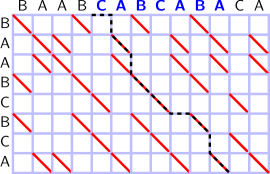
Example 4.6.
Figure 4.1 shows the alignment dag for strings , . All edges are directed left-to-right and top-to-bottom. The diagonal edges of score are not shown. The colour of the remaining edges indicates their scores: blue (respectively, red) corresponds to edge score (respectively, ). ■
A particular special case of an alignment dag is the full-mismatch dag, which consists entirely of mismatch cells. This dag can be obtained as the alignment dag of a pair strings that have no characters in common. Another special case is the full-match dag, which consists entirely of match cells. This dag can be obtained as the alignment dag of a pair of strings over an alphabet of a single character, or, alternatively, a pair of strings, one of which consists entirely of wildcard characters.
Given a pair of strings , , their semi-local common subsequences correspond to boundary-to-boundary paths in the alignment dag . In particular, a common string-substring, suffix-prefix, prefix-suffix, or substring-string subsequence corresponds, respectively, to a top-to-bottom, left-to-bottom, top-to-right, and left-to-right path. The length of a subsequence is equal to the total score of the corresponding path. The semi-local LCS problem is therefore equivalent to finding the maximum path scores of the following four types:
| (4.1) | ||||
| (4.2) | ||||
| (4.3) | ||||
| (4.4) |
where , , and the score maxima are taken across all paths between the given endpoints. The diagonal edges with score in mismatch cells do not affect maximum node-to-node scores, and can therefore be ignored.
Example 4.7.
In Figure 4.1, the highlighted top-to-bottom path corresponds to the string-substring LCS score . ■
Finding the maximum boundary-to-boundary path scores in an alignment dag is equivalent to finding the corresponding distances in an undirected graph, obtained from the alignment dag by assigning length to vertical and horizontal edges, assigning lengths and to diagonal edges in match and mismatch cells respectively, and ignoring edge directions. The problem thus becomes a special case of the problem to find distances between boundary nodes and all nodes in a planar graph. In the case a grid-diagonal dag with arbitrary real weights, this problem has been studied by Schmidt [157]. In the still more general case of an arbitrary real-weighted undirected planar graph, the problem has been studied by Klein [114] and Cabello and Chambers [41]. These more general algorithms are slower than the ones presented in this work, where we exploit both the grid-diagonal structure of the dag, and the discreteness of edge lengths.
The analysis of the four different path types (4.1)–(4.4) can be simplified by padding string with wildcard characters on both sides, and then considering paths in the alignment dag for string over against the padded string over .
Definition 4.8.
Given strings , , the corresponding semi-local score matrix111These matrices are called “DIST matrices” e.g. in [157, 57], and “score matrices” in [164]. Our current terminology is chosen to reflect the semi-local score-maximising nature of the matrix elements, while avoiding confusion with pairwise substitution score matrices used in comparative genomics (see e.g. [107]). is a matrix over , defined by
where , , and the maximum is taken across all paths between the given endpoints , in the padded alignment dag . If , we have . By convention, if , then we let . □
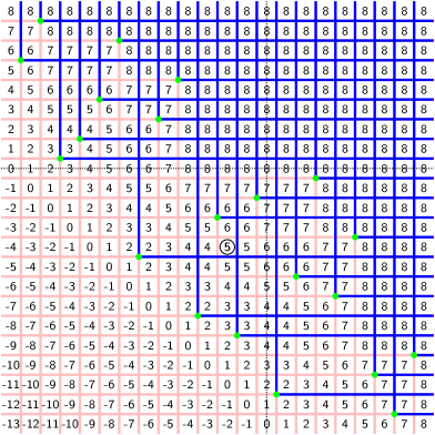
Example 4.9.
Figure 4.2 shows the matrix , giving all semi-local LCS scores for strings , as in the previous examples. The entry is circled. ■
The solution for each of the four components of the semi-local LCS problem in Definition 4.3 can now be obtained from (4.1)–(4.4) as follows:
where , .
The key property of semi-local score matrices is captured by the following theorem.
Theorem 4.10.
Given strings , , the corresponding semi-local score matrix is unit-anti-Monge. More precisely, we have
where is a permutation matrix over . In particular, string is a subsequence of substring for some , if and only if . □
Proof.
For any crossing pair of highest-scoring paths, and , where , , there exists a non-crossing pair of paths and of at least the same total score, which can be obtained by rearranging the edges in the paths. Therefore, we have
for all , , hence , and matrix is anti-Monge.
Let . From the above, matrix is Monge. We have
for all , , hence is simple. Furthermore, we have
| (definitions of and ) | |||
| (cancellation) | |||
for all . Analogously,
for all . By Lemma 2.11, matrix is simple unit-Monge. Therefore, , where is a permutation matrix. The second equality in the theorem statement is now straightforward from the definitions. ■
The intuition behind Theorem 4.10 is as follows. Let be a substring of , and consider its LCS score against string . If substring is extended at either end by one character, the LCS score is either unchanged, or increased by , depending on whether or not the new character of can be usefully matched to a character of . The unit-anti-Monge property of matrix describes the fact that, as substring grows in size, so does the number of obstacles to useful matching of characters. Each obstacle, in other words a “critical point” at which a useful match become useless, corresponds to a nonzero in the permutation matrix . However, this is only very general intuition: in fact, the notion of a “useful match” is not absolute, but depends on the choice of a particular highest-scoring path through the alignment dag.
Theorem 4.10 and its proof hold more generally for any grid-diagonal dag, not necessarily obtainable as an alignment dag of any particular pair of strings. However, the given form of the theorem will be sufficient for the rest of this work.
The key idea of our approach is to view Theorem 4.10 as a description of an implicit solution to the semi-local LCS problem: the semi-local score matrix is represented implicitly by (the nonzeros of) the permutation matrix .
Definition 4.11.
Given strings , , the semi-local seaweed matrix is a permutation matrix over , defined by Theorem 4.10. □
Definition 4.11 leads to the following interpretation of Theorem 4.10. The LCS score for string against substring is determined by the length of , and by the number of nonzeros in that are -dominated by the point . Alternatively, the same LCS score is determined by the length of string , and by the number of nonzeros in that -dominate the point .
Example 4.12.
Figure 4.2 shows the unit-anti-Monge property of matrix by the coloured grid pattern: red (respectively, blue) lines separate matrix elements that differ by (respectively, by ). The nonzeros of the semi-local seaweed matrix over are shown by green bullets.
Nonzeros of that are -dominated by the point correspond to the green bullets lying below-left of the circled entry. There are exactly two such nonzeros, therefore , and we have .
Nonzeros of that -dominate the point correspond to the green bullets lying above-right of the circled entry. There are exactly three such nonzeros, therefore , and we have . ■
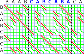
A semi-local seaweed matrix can be naturally identified with a reduced seaweed braid of width (or, more precisely, with a family of equivalent reduced seaweed braids). As we show in the following section, divide-and-conquer solutions to the semi-local LCS problem generally correspond to implicit distance multiplication of seaweed matrices, and therefore also to the multiplication of the corresponding seaweed braids.
Example 4.13.
Figure 4.3 shows matrix as a reduced seaweed braid of width , laid out directly on the alignment dag . The nonzeros correspond to seaweeds, laid out as paths in the dual graph. We say that a seaweed goes from to , if it originates between the nodes and , and terminates between the nodes and . In particular, every nonzero , where , is represented by a seaweed going from to . The remaining seaweeds, originating or terminating at the sides of the dag, correspond to nonzeros , where either , or , or both. For the purposes of this example, the specific layout of the seaweeds between their endpoints is not important. However, this layout will become meaningful in the context of the algorithms described in the next chapter.
The full set of nonzeros corresponds to the full set of seaweeds in Figure 4.3. The two nonzeros that are -dominated by the point correspond to the two seaweeds, going from to and from to . These two seaweeds fit completely between the two dashed vertical lines and . The three nonzeros that -dominate the point correspond to the three seaweeds going from to the right boundary, from to , and from to the right boundary. These three seaweeds pierce both dashed vertical lines. ■
When talking about semi-local score and seaweed matrices, we will sometimes omit the qualifier “semi-local”, as long as it is clear from the context.
The definitions of score and seaweed matrices are not symmetric with respect to the order of the input strings. The precise relationship between score matrices , , and between seaweed matrices , , is given by the following lemma.
Lemma 4.14.
Given input strings , , we have
for all , , and
for all , . □
Proof.
Straightforward by definitions. ■
4.4 Seaweed submatrix notation
The four individual components of the semi-local LCS problem correspond to a partitioning of both the score matrix and the seaweed matrix into submatrices. It will be convenient to introduce a special notation for these submatrices as follows:
For example, we have , which is the matrix of all string-substring LCS scores for strings , . Note that the four resulting submatrices of overlap by one row/column at the boundaries (in particular, the global LCS score belongs to all four score submatrices), while the corresponding submatrices of are disjoint:
Definition 4.15.
Given strings , , the corresponding suffix-prefix, substring-string, string-substring and prefix-suffix score (respectively, seaweed) matrices are the submatrices , , , (respectively, , , , ). □
Similarly to the full semi-local seaweed matrix, its component seaweed submatrices can be processed into an efficient data structure of Theorem 2.15 for answering individual semi-local score queries.
Example 4.16.
Figure 4.2 shows by thin dotted lines the partitioning of and into submatrices of Definition 4.15. The suffix-prefix, substring-string, string-substring and prefix-suffix submatrices are respectively on the top-left, top-right, bottom-left and bottom-right. The elements of lying directly on the dotted lines are shared by the bordering score submatrices. Note that the substring-string score submatrix and seaweed submatrix are both filled with a constant value ( and , respectively); this is due to the fact that the whole string is a subsequence of . ■
The nonzeros of each seaweed submatrix introduced in Definition 4.15 can be regarded as an implicit solution to the corresponding component of the semi-local LCS problem. Similarly, by considering only three out of the four submatrices, we can define an implicit solution to the extended string-substring (respectively, substring-string) LCS problem.
Definition 4.17.
Given strings , , we define the extended string-substring (respectively, substring-string) seaweed matrix over as
□
The extended string-substring seaweed matrix contains at least and at most nonzeros. Note that for , the number of nonzeros in is at most , which is convenient when is large. Analogously, for , the number of nonzeros in the extended substring-string matrix is at most , which is convenient when is large.
Let string of length be a concatenation of two fixed strings: , where , are nonempty strings of length , respectively, and . A substring of the form with , will be called a cross-substring. A cross-substring that is either a suffix of , or a prefix of (i.e. with either , or ), will be called degenerate. In other words, a cross-substring of consists of a suffix of and a prefix of ; a cross-substring is non-degenerate, if and only if both of these are non-empty. A cross-substring that is a prefix or a suffix of will be called a cross-prefix and a cross-suffix, respectively. Given string of length that is a concatenation of two fixed strings, , cross-substrings of are defined analogously.
Definition 4.18.
Given strings and , the corresponding cross-semi-local score matrix is the submatrix
Symmetrically, given strings and , the corresponding cross-semi-local score matrix is the submatrix
The cross-semi-local seaweed matrices are defined analogously:
□
A cross-semi-local score matrix represents the solution of a restricted version of the semi-local LCS problem. In this version, instead of all substrings (prefixes, suffixes) of string (respectively, ), we only consider cross-substrings (cross-prefixes, cross-suffixes). At the submatrix boundaries and , cross-substrings of string degenerate to suffixes of and prefixes of ; in particular, cross-prefixes and cross-suffixes of degenerate respectively to the whole and . The submatrix boundaries and correspond to similarly degenerate cross-substrings of string . Submatrix elements on these boundaries will also be called degenerate.
Occasionally, we will use cross-semi-local score and seaweed matrices in combination with the superscripted submatrix notation, introduced earlier in this section. In such cases, the range of the resulting matrix will be determined by the intersection of the ranges implied by the superscript and the subscript. For example, matrix is the string-cross-substring score matrix, i.e. the matrix of all LCS scores between string and all cross-substrings of string .
In all the above definitions, the seaweed matrices can be used to give an implicit representation for the corresponding score matrices, just as the full seaweed matrix does for the full score matrix .
4.5 Alignment dag composition
We now combine all the concepts and techniques introduced in previous sections to provide a mechanism for string comparison in a divide-and-conquer framework.
Let , be nonempty strings of length , respectively. We consider the semi-local LCS problem on a concatenation string of length against a fixed string of length .
The alignment dag consists of alignment subdags , , sharing a horizontal row of nodes and edges, which is simultaneously the bottom row of and the top row of . We will say that dag is the composite of dags and .
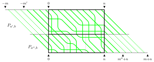
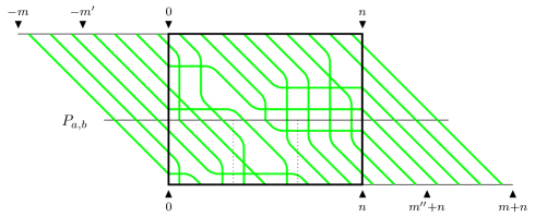
Our goal is, given the seaweed matrices , , to compute the composite seaweed matrix . It turns out that this problem can be solved efficiently by the techniques of Chapter 3.
Theorem 4.19.
The composite string-substring (respectively, semi-local) seaweed matrix can be obtained from the respective original seaweed matrices as
| (4.5) | |||
| (4.6) |
Here, the dimensions of the offset identity submatrices are chosen to conform to the dimensions of the product. □
Proof.
By Theorem 4.10, we have
for all , . Three cases are possible, based on the partitioning of the index ranges.
Example 4.20.
Theorem 4.21.
Given a pair of seaweed matrices, the corresponding composite seaweed matrix can be computed in the following time:
| Type | Input | Output | Time |
|---|---|---|---|
| string-substring | , | ||
| extended string-substring | , | ||
| cross-semi-local | |||
| semi-local | , |
Here, . □
Proof.
We prove the statement in the final row of the table; the proof for other rows is analogous.
We will represent the product (4.6) by a product of seaweed braids. To achieve such a representation, we need to extend the notion of seaweed braid multiplication to pairs of braids whose index ranges are not identical, but have a partial overlap. Consider two seaweed braids of size , respectively, whose index ranges overlap over a range of width . The product of such seaweed braids can be defined naturally as follows. We join up the seaweeds across the overlap, and extend each of the remaining seaweeds either upwards or downwards by a straight vertical line, forming the resulting product braid of width . By Theorem 3.16, such a staggered seaweed product can be computed in time .
In the setting of the current theorem, the semi-local seaweed matrices , correspond each to a seaweed braid of width , respectively. The two braids overlap along the common boundary of the two dags; the width of the overlap is , so the width of the (generally non-reduced) product seaweed braid is .
Suppose . Then, as discussed above, the seaweed product of width can be computed directly in time .
We may now assume without loss of generality that . Assume, also without loss of generality, that is an integer. We partition the dag into square blocks of size . Consider the seaweed braid of width , corresponding to matrix . It is now straightforward to decompose this seaweed braid into a staggered product of seaweed braids of width , so that each pair of successive braids in this product overlap over an interval of width . Given the matrix , the seaweed matrices for all the braids in the product can easily be obtained in time .
We now compute the product (4.6) by first performing successive multiplications of the seaweed braid corresponding to by each of the braids in the decomposition of . The resulting running time is . ■
Example 4.22.
Figure 4.4 illustrates the proof of Theorem 4.21 as follows. Decomposition of the seaweed braid corresponding to matrix into blocks is shown in Subfigure 4.4a by thin dotted lines. Clearly, the whole seaweed braid for can be obtained from by successive multiplication with staggered block subbraids of , block-by-block. Subfigure 4.4b shows the resulting seaweed braid for the product matrix . ■
Chapter 5 The seaweed method
In this chapter, we develop a simple and efficient algorithm for the semi-local LCS problem, called the seaweed combing algorithm. We then give some of the algorithm’s modifications and applications.
This chapter is organised as follows. In Section 5.1, we describe the main version of the seaweed combing algorithm, and in Section 5.2, its micro-block speedup. In Sections 5.3 and 5.4, we apply the seaweed combing algorithm to solving several incremental and blockwise versions of the semi-local LCS problem. In Section 5.5 we give algorithms for the window LCS and cyclic LCS problems, and in Section 5.6 for the longest repeating subsequence problem. All our algorithms match, improve on, and/or generalise the existing algorithms.
5.1 Seaweed combing
A classical solution to the global LCS problem on input strings and is given by the dynamic programming algorithm, discovered independently by Needleman and Wunsch [141] (without an explicit analysis), and by Wagner and Fischer [175]. This algorithm solves in fact the more general prefix-prefix LCS problem, which consists in computing the LCS scores for all prefixes of string against all prefixes of string . The algorithm assumes a character comparison model that only allows comparison outcomes “equal” and “unequal”, and the unit-cost RAM computation model; it runs in time . The solution to the prefix-prefix LCS problem can be used to trace back (i.e. to obtain character by character) the actual LCS of strings and in time proportional to the size of the output (i.e. the length of the output subsequence). A memory-saving recomputation technique by Hirschberg [94] can be applied to achieve LCS traceback in the same asymptotic time, but in a linear amount of memory.
The semi-local LCS problem can be solved naively by computing the LCS score for each semi-local substring pair (string-substring, etc.) independently by the classical dynamic programming algorithm, in overall time . By making use of all the prefix-prefix LCS scores produced by each run of the classical algorithm, this can be improved to . Based on the ideas of Schmidt [157], Alves et al. [11] gave an algorithm for the string-substring LCS problem. Their algorithm solves in fact the more general prefix-substring LCS problem, which consists in computing an implicit representation of the LCS scores for all prefixes of string against all substrings of string . The algorithm runs in time . It therefore extends the functionality of the standard dynamic programming LCS algorithm (prefix-substring instead of just prefix-prefix), while matching its asymptotic running time.
We now give a simple and efficient algorithm for the semi-local LCS problem, which extends still further the functionality of the above algorithms, while matching their model assumptions and asymptotic running time. We call it the seaweed combing algorithm, since it can be interpreted in terms of combing (i.e. removing double crossings from) seaweed braids.
Algorithm 5.1.
(Semi-local LCS: Seaweed combing)
strings , of length , , respectively.
nonzeros of semi-local seaweed matrix .
We obtain the output matrix by constructing its corresponding reduced seaweed braid of width , laid out within the cells of the alignment dag . Individual seaweeds within the braid will be identified by their starting index at the top boundary of the padded alignment dag .
We initialise the seaweed braid as a composition of elementary seaweed braids, each laid over a single cell of . An elementary braid in a match (respectively, mismatch) cell consists of two non-crossing (respectively, crossing) seaweeds. The composition of all elementary braids is a generally unreduced seaweed braid of width , laid over the full dag . By Theorem 4.19, an equivalent reduced seaweed braid corresponds to the semi-local seaweed matrix .
We now need to comb the initial unreduced seaweed braid, in order to obtain an equivalent reduced one. The combing is performed by sweeping the cells of the alignment dag from left to right and from top to bottom, either in the lexicographic order, or in any other total order compatible with the -dominance partial order of the cells.
For each cell, we consider the two seaweeds passing through it. The two seaweeds initially cross within the cell, if and only if it is a mismatch cell. The new layout for the two seaweeds within the current cell is decided as follows. In a match cell, we always leave the seaweeds uncrossed. In a mismatch cell, we first determine whether the two crossing seaweeds have ever crossed previously (in terms of the cells’ -dominance order) in the alignment dag. This check can be performed efficiently by comparing the starting indices of the two current seaweeds. If the current pair of seaweeds have never crossed previously, we keep their crossing in the current cell. However, if the two seaweeds have crossed previously, we undo (“comb away”) their crossing in the current cell. We then move on to the next cell in the sweeping order.
From the definition of the seaweed monoid (Definition 3.20), it is easy to see that each step is an equivalence transformation on the current seaweed braid. Hence, the resulting seaweed braid is equivalent to the initial one. Furthermore, since our procedure never allows a given pair of seaweeds to cross twice, the resulting seaweed braid is reduced, and gives us the nonzeros of the output matrix .
Within a cell, both the crossing check and the update run in time . Therefore, the overall running time of the algorithm is .
Note that we never need to store the full seaweed braid explicitly. For each seaweed, we only need to store its starting index, and its index on the current frontier of processed cells. Therefore, the overall memory cost of the algorithm is . ■
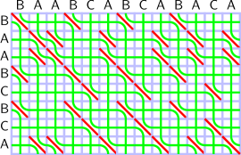
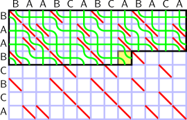
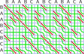
Example 5.2.
Subfigure 5.1a shows the initial state of the seaweed braid, obtained by direct composition of elementary braids in all the individual cells. The dag is then swept in the top-to-bottom, left-to-right lexicographic cell order, which is compatible with -dominance of the cells.
Subfigure 5.1b shows a snapshot of some intermediate state of the seaweed braid. The dag area that has already been processed is shown by the dark border; the current cell is shaded in yellow. Since the two seaweeds passing through the current cell have previously crossed, their crossing has been undone in the current cell.
Recall that the dag cells in Algorithm 5.1 can be swept in any order compatible with -dominance of the cells. Note that, irrespective of the sweeping order, the algorithm ends up computing a reduced seaweed braid (and therefore, implicitly, the semi-local seaweed matrix) for each prefix of string against whole string , and for the whole string against each prefix of string . By building an appropriate data structure for querying these implicit matrices, we obtain a solution to the more general prefix semi-local LCS problem, which incorporates the (ordinary) semi-local LCS problem, and consists in computing an implicit representation of the LCS scores for all prefixes of string against all substrings of string , and for all substrings of string against all prefixes of string .
As in the standard dynamic programming LCS algorithm, the solution to the prefix semi-local LCS problem can be used to trace back the actual LCS corresponding to any prefix semi-local (i.e. prefix-substring or substring-prefix) LCS query, in time proportional to the size of the output. A technique similar to the one by Hirschberg [94] can also be applied to achieve prefix semi-local LCS traceback in the same asymptotic time, but in a linear amount of memory.
Assuming the “equal/unequal” character comparison model, Aho et al. [2] gave a lower bound of on the solution running time of the (global) LCS problem (see also a survey by Bergroth et al. [26]). Both the standard dynamic programming LCS algorithm, and the seaweed combing algorithm (Algorithm 5.1) match this lower bound, and are therefore asymptotically optimal in this model.
5.2 The micro-block speedup
In the previous section, we developed a semi-local LCS algorithm running in time , assuming the character comparison model that only allows comparison outcomes “equal” and “unequal”. We now aim for an asymptotically faster algorithm. In such a situation, we cannot afford to perform all the pairwise comparisons of characters from each string. Therefore, it is natural to switch to a more powerful comparison model, where the alphabet is a totally ordered set, and comparison outcomes are “less than”, “equal” and “greater than”. The “missing” comparisons can be obtained by transitivity. In this model, we no longer need to process every dag cell individually, so algorithms with running time become possible111This holds true even if the computation model assumption is weakened, so that character comparisons and arithmetic operations are charged using the log-cost RAM model. However, for uniformity we will stick to our original assumption of the unit-cost RAM model..
A classical LCS computation speedup originates from a matrix multiplication method by Arlazarov et al. [18], often nicknamed the “four Russians method”. In this work, we call it the micro-block speedup, adopting the terminology of Bille and Gørtz [30]. The main idea of this method is to sweep the alignment dag in regular micro-blocks of a small, suitably chosen size, such that running time can be saved by precomputing all possible micro-block updates in advance. Without loss of generality, we assume that . By applying the micro-block speedup to the classical dynamic programming algorithm, Masek and Paterson [132] gave an algorithm for the (global) LCS problem running in time for a constant-size alphabet222The original algorithm by Masek and Paterson [132] runs in time for a constant-size alphabet in the log-cost RAM model. The unit-cost RAM version of the algorithm was given in [177, 29].. An alternative approach to subquadratic LCS computation was developed by Crochemore et al. [58].
An extension of the micro-block subquadratic LCS algorithm to an alphabet of unbounded size, running in time , was suggested by Paterson and Dančík [143], and fully developed by Bille and Farach-Colton [29]. In this extension, a second, coarser level of alignment dag partitioning is introduced. The blocks of this second level, called macro-blocks, are used for reducing the effective alphabet size, maximising the number of input string characters that fit into a machine word for each micro-block update.
We now give an algorithm for semi-local LCS running in subquadratic time, which makes a slight improvement on Algorithm 5.1. The algorithm uses the two-level micro-block method, similar to the global LCS algorithm of [29], and matches it in running time. At the same time, our algorithm provides a substantially more detailed string comparison. However, in contrast to the global LCS algorithms, our algorithm does not allow any further speedup in the case of a constant alphabet size.
Algorithm 5.3.
(Semi-local LCS: Seaweed combing with micro-block speedup)
strings , of length , , respectively; we assume .
nonzeros of semi-local seaweed matrix .
Without loss of generality, we may assume that the alphabet size is at most , and that the characters are encoded by half-integers in the range . We call two strings of equal length isomorphic, if one can obtained from the other by a permutation of the alphabet.
We process the alignment dag in square micro-blocks of size
where the logarithms are base 2. Similarly to Algorithm 5.1, we start with an initial seaweed braid of width , obtained as a composite of elementary seaweed braids in individual cells.
We then transform the seaweed braid by incremental micro-block combing into an equivalent reduced seaweed braid, corresponding to the output matrix . The algorithm sweeps the alignment dag in an arbitrary order compatible with the -dominance order of the micro-blocks. For each micro-block, we perform an update on the current seaweed braid.
Consider a micro-block defined by the input substrings , , where , . Let . A total of seaweeds pass through the current micro-block. A micro-block can be regarded as a function, parameterised by the current input substrings, and performing an update on the permutation matrix , corresponding to a subbraid of width defined by the micro-block. The states of matrix before and after the update will be called the micro-block’s input matrix and output matrix, respectively. Note that both of these are permutation matrices, and therefore can be represented implicitly by their nonzeros.
The alignment dag can be swept in an arbitrary order compatible with the -dominance partial order of the micro-blocks. Combined with precomputation, this is already sufficient to obtain a subquadratic algorithm. However, in order to achieve higher speedup, we introduce a second level of macro-blocks of size
We define a macro-block’s input and output matrices similarly to a micro-block’s ones.
The characters of a macro-block’s defining input substrings are encoded by values in the range . The macro-block’s input and output matrices are represented by the row and column indices of the nonzeros; the natural range of these indices is also . In order to perform the computation efficiently, we remap each of these ranges to a smaller range before passing the values to the micro-block level. The range remapping preserves the linear order of the values (both characters and matrix indices).
We process each macro-block as follows. First, we obtain its defining substrings and the input matrix; overall, we have characters and index values for the macro-block. We then remap both the characters and the index values from to by removing unused values from the range, while preserving the relative order of the remaining values. This remapping requires sorting of the values, and can be performed in time . We then sweep the current macro-block by micro-blocks, in an arbitrary order compatible with the -dominance partial order of the micro-blocks. For each micro-block, we obtain its defining input substrings and the input matrix; overall, we have values for the micro-block of size . We then apply a precomputed update to the micro-block’s input matrix .
The micro-block’s defining substrings and the input matrix consist each of values, ranging over . For each of the at most possible combinations of the input character and index values, the output index values resulting from the update are precomputed in advance, using Algorithm 5.1.
The algorithm maintains the same invariant as Algorithm 5.1: the current seaweed braid is equivalent to the initial one, and corresponds to the semi-local LCS problem on the dag . Therefore, at the end of the sweep, we obtain a reduced seaweed braid corresponding to the output matrix .
In the precomputation stage, there are at most problem instances, each of which runs in time . Therefore, the running time of the precomputation is
which is negligible, compared to the subsequent main computation stage.
In the main computation stage, there are micro-block update steps. The micro-block’s defining substrings and input-output matrices are each represented by values in the range . The full micro-block data are of size
and hence fit into a constant number of machine words. Therefore, the total running time of the algorithm is
■
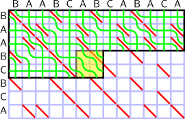
Example 5.4.
5.3 Incremental LCS
We now begin to explore the applications of the seaweed method. First, we consider on-line string comparison. In this framework, rather than dealing with a pair of fixed input strings, we consider either one or both strings to be variable. These variable string(s) are subject to updates; several different models of string updating may be considered. The goal of an on-line LCS algorithm is to maintain a data structure that will store the LCS score for the input strings, and will allow efficient on-line updates of this score. We denote by , denote the current state of each input string, and by , their respective current size.
Appending characters.
The simplest possible model of string updating is by appending a character at the end of an input string. The classical dynamic programming LCS algorithm [141, 175] maintains an array of all prefix-prefix LCS scores. Such an array can be efficiently updated whenever a character is appended (but not prepended) to either of the input strings. The running time of this on-line version of the classical dynamic programming algorithm is (respectively, ) per update of string (respectively, ).
Appending/prepending characters.
Another possible model for string updating is to allow both appending a character at the end, and prepending a character at the beginning of a string. This updating model is assumed by the incremental LCS problem, introduced by Landau et al. [122] and by Kim and Park [113]. The problem asks to maintain the LCS score for a fixed string against a variable string , updated on-line by appending and/or prepending characters. Works [122, 113] gave algorithms for the incremental LCS problem with worst-case time per update of string .
The more general fully-incremental LCS problem, was introduced by Ishida et al. [102]. Here, both strings can be updated on-line by appending and/or prepending characters at either end. Work [102] gave an algorithm for the fully-incremental LCS problem, with worst-case time (respectively, ) per update of string (respectively, ).
A new algorithm for the fully-incremental LCS problem, matching the above algorithms in running time, can be obtained by a straightforward generalisation of Algorithm 5.1 (seaweed combing) as follows. Our dynamic LCS data structure will consist of the nonzeros of semi-local seaweed matrix . Whenever a new character is prepended or appended to string (respectively, ), this seaweed matrix is updated by processing a new row of cells along the top or bottom boundary (respectively, a new column of cells along the left or right boundary) of the alignment dag . This amounts to the multiplication of seaweed braids corresponding to alignment dags of size and (respectively, and ). A product of such seaweed braids can be computed in time (respectively, ) by Theorem 4.21. Having computed the product, it is also straightforward to update the value of the LCS in the same asymptotic running time. Therefore, the overall running time per update is (respectively, ) per update of string (respectively, ).
5.4 Blockwise LCS
To demonstrate another natural application of the seaweed method, let us consider the following generalisation of string comparison. Suppose that instead of individual characters, the input string is composed of character blocks, taken from a pre-specified set of admissible blocks (for example, a list of frequently occurring words in a text). The set of admissible blocks is known in advance, and off-line preprocessing of the blocks against input string is allowed.
Block decomposition of strings is very common in string compression. In this section, we are only dealing with the most general case of such decomposition; we will consider specific string compression models in Chapter 9.
We denote by the number of blocks in string , while keeping the notation for its total number of characters. A block may consist of a single character, therefore such blockwise string comparison generalises ordinary string comparison. On the other hand, a block may be long; in such a case, our goal is to process the block quickly, ideally in the same time as it takes to process a single character in string .
Given a string of blocks , and a string of ordinary characters , the blockwise LCS problem asks for their LCS score. Likewise, the blockwise semi-local LCS problem asks for their implicit semi-local LCS scores, represented by the seaweed matrix . We can solve both problems naively, by running Algorithm 5.1 while ignoring the block structure of string , in time .
A special case of the blockwise LCS problem was introduced by Landau and Ziv-Ukelson [124] as the common-substring LCS problem (see also [57]). In this version of the problem, there is only a single non-trivial admissible block of length , called common substring. The algorithm of [124] preprocesses the common substring against string in time , and then solves the common-substring LCS problem in time .
The seaweed method allows us to solve the blockwise LCS and the blockwise semi-local LCS problems efficiently as follows.
Preprocessing.
Blockwise LCS.
Let us define the score vector over as . We compute this vector incrementally as follows. Suppose we have computed the vector , and let , where is an admissible block. Then we have , where matrix has been obtained in the preprocessing phase. This implicit vector-matrix distance product can be computed by Theorem 3.15 in time . The overall running time is .
Blockwise semi-local LCS.
We compute the seaweed matrix incrementally, starting from the precomputed matrix for an arbitrary block of string . Suppose we have computed the matrix , and let , where is an admissible block (the case is dealt with analogously). Then we have , where, as before, matrix has been obtained in the preprocessing phase. This implicit matrix distance product can be computed by Theorem 4.21 in time , where is the length of block . The overall running time is , where is the maximum size of an admissible block.
Symmetric blockwise (semi-local) LCS.
Let us consider the symmetric version of the above problems, where input strings and are both composed of admissible blocks, on which preprocessing is allowed. In this setting, the preprocessing runs in time for each pair of blocks of lengths , . The blockwise LCS problem can then be solved in time , where and is the number of blocks in string and , respectively. The blockwise semi-local LCS problem can be solved in time , where is the maximum size of an admissible block.
Incremental blockwise (semi-local) LCS.
We can also consider the incremental versions of the blockwise LCS and semi-local LCS problems, generalising the incremental (semi-local) LCS problem considered in Section 5.3. Both input strings are considered to be variable; either string can be updated by appending a block on the right, or prepending a block on the left. The block-incremental LCS problem asks to maintain a data structure that will store the LCS score for the input strings, and will allow efficient on-line updates of this score.
The incremental blockwise (semi-local) LCS problem can be solved by the above algorithms as follows. The algorithm for the blockwise LCS problem takes time (respectively, ) to process a block appended to string (respectively, ); here, blocks can only be appended to either string on the right. The algorithm for the blockwise semi-local LCS problem takes time (respectively, ) to process a block either appended or prepended to string (respectively, ); blocks can be appended (prepended) both on the right or on the left.
5.5 Window LCS and cyclic LCS
Given a fixed parameter , we call a substring of length a -window in the corresponding string. Given strings , , and a window length , the window LCS problem asks for the LCS score of the whole string against every -window in string .
Using the seaweed method, we are now able to give a simple efficient algorithm for the window LCS problem. First, we run Algorithm 5.3 (micro-block seaweed combing) on strings , obtaining the semi-local seaweed matrix . Then, we perform string-substring LCS score queries for whole against every -window of . This can be done efficiently as a diagonal batch query via Theorem 2.17. The overall running time is dominated by the call to Algorithm 5.3, which runs in time .
The following problem can also be solved as a special case of the window LCS problem. Given strings , of length , respectively, the cyclic LCS problem asks for the highest LCS score of against all cyclic shifts of (equivalently, all cyclic shifts of against , or all cyclic shifts of both strings against each other). Cyclic string comparison has been considered by Maes [129], Bunke and Bühler [36], Landau et al. [122], Schmidt [157], Marzal and Barrachina [131]. The algorithms of [122, 157] solve the cyclic LCS problem in worst-case time .
We now give a simple algorithm for the cyclic LCS problem, improving on the existing algorithms by the micro-block speedup. First, we solve the window LCS problem on string against string (a concatenation of string with itself), which is of length , with window size . We then take the maximum LCS score across all windows. The overall running time is still dominated by the call to Algorithm 5.3, which runs in time .
5.6 Longest repeating subsequence
Given a string of length , the longest repeating subsequence problem asks for the length of the longest subsequence of that is a square, i.e. a concatenation of two identical strings.
This problem has been considered under the name “longest tandem scattered subsequence problem” by Kosowski [117], who gave an algorithm running in time .
Using the seaweed method, we are now able to give a new algorithm for the longest repeating subsequence problem, improving on the existing algorithm by the micro-block speedup. First, we run Algorithm 5.3 (micro-block seaweed combing) on string against itself, obtaining the semi-local seaweed matrix in time . Then, we perform prefix-suffix LCS score queries for every possible non-trivial prefix-suffix decomposition of ; this can be done in time per query by Theorem 2.17. Finally, we take the maximum score among all the queries. The overall running time is .
Chapter 6 Weighted string comparison
In this chapter, we generalise our techniques developed for the unweighted semi-local LCS problem to rational-weighted semi-local string comparison.
This chapter is organised as follows. In Section 6.1, we introduce weighted string alignment, and describe the blow-up technique for rational-weighted alignment. In Section 6.2, we use the framework of weighted alignment to obtain algorithms for several versions of the approximate pattern matching problem.
6.1 Weighted scores and edit distances
The concept of LCS score is generalised by that of (weighted) alignment score (see e.g. [104]). An alignment of strings , is obtained by putting a subsequence of into one-to-one correspondence with a (not necessarily identical) subsequence of , character by character and respecting the index order. The corresponding pair of characters, one from and the other from , are said to be aligned. A character that is not aligned against a character of another string is said to be aligned against a gap in that string. Each of the resulting character alignments is given a real weight:
-
a pair of aligned matching characters has weight ;
-
a pair of aligned mismatching characters has weight ;
-
a gap-character or character-gap pair has weight ; it is normally assumed that (i.e. this weight is in fact a penalty).
The intuition behind the weight inequalities is as follows: aligning a matching pair of characters is always better than aligning a mismatching pair of characters, which in its turn is never worse than leaving both characters unaligned (aligned against a gap).
Definition 6.1.
The (weighted) alignment score for strings , is the maximum total weight across all possible alignments of against . □
Example 6.2.
The LCS alignment score is given by
A slightly more sophisticated alignment score, intended to penalise gaps in DNA sequence alignment, is given by
Another alignment score used for DNA sequence comparison [47, Section 1.3] is given by
■
Definition 6.3.
We define the semi-local (weighted) alignment score problem and its component subproblems (string-substring alignment score, etc.) by straightforward extension of Definition 4.3, replacing the LCS score by (weighted) alignment scores. □
The concepts of alignment dag and score matrix, which we introduced in Chapter 4 for unweighted alignments, can also be naturally extended to the weighted case. To distinguish between the weighted and unweighted cases, we will use the script font (e.g. , ) in the weighted case, keeping the ordinary font (, ) for the unweighted case.
Definition 6.4.
We define the weighted alignment dag by straightforward extension of Definition 4.5, where diagonal match edges, diagonal mismatch edges, and horizontal/vertical edges have weight , , , respectively. □
Definition 6.5.
We define the semi-local (weighted) score matrix by straightforward extension of Definition 4.8. A semi-local alignment score corresponds to a boundary-to-boundary highest-scoring path in the padded weighted alignment dag . □
Matrix is anti-Monge. However, in contrast with the unweighted case, it is not necessarily unit-anti-Monge.
Given an arbitrary set of alignment weights, it is often convenient to normalise them so that . To obtain such a normalisation, first observe that, given a pair of strings , , and arbitrary weights , , , we can replace the weights respectively by , , , for any real . This weight transformation increases the score of every global alignment (top-left to bottom-right path in ) by . Therefore, the relative scores of different global alignment paths do not change. In particular, the maximum global alignment score is attained by the same path for all values of . By taking , and dividing the resulting weights by , we achieve the desired normalisation. (A similar method is used by Rice et al. [149]; see also [91, 107].)
Definition 6.6.
Given original weights , , , the corresponding normalised weights are
The resulting normalised score is
where is the original alignment score. This original score can be restored from the normalised one by reversing the normalisation: . □
Example 6.7.
In Example 6.2, the LCS score is already normalised. The other two scores correspond to normalised scores with weights , (respectively, ), and . ■
As discussed above, maximising the normalised global alignment score is equivalent to maximising the original score , for fixed string lengths and . However, more care is needed when it is required to maximise the alignment score across substrings of different lengths, which is typical for various approximate string matching problems. In such cases, explicit conversion from normalised weights to original weights will be necessary prior to the maximisation.
In this work, we will mostly restrict ourselves to character alignment weights that satisfy the following rationality condition.
Definition 6.8.
A set of character alignment weights will be called rational, if all the weights are rational numbers. □
For a rational set of alignment weights, the corresponding normalised weights (in particular, the only non-trivial normalised weight ) are also rational. Given such a rational set of normalised weights, the semi-local alignment score problem on strings , can be reduced to the semi-local LCS problem by the following blow-up procedure. Let , where , are positive natural numbers. We transform input strings , of lengths , into new blown-up strings , of lengths , . The transformation consists in replacing every character in each of the strings by a substring of length (recall that $ is a special guard character, not present in the original strings). We have
for all , , where the matrix is defined by the normalised scores on the original strings , , and the matrix by the LCS scores on the blown-up strings , . Using this reduction, we are able to apply the techniques of semi-local LCS to the more general semi-local alignment score problem, assuming that all weights are rational and that is constant.
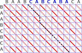
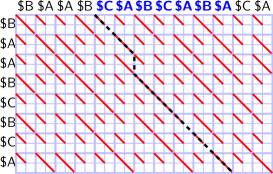
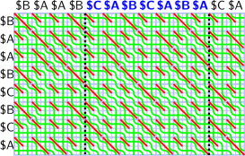
Example 6.9.
Figure 6.1 shows semi-local weighted alignment of strings , , using normalised alignment weights , , .
Subfigure 6.1a shows the alignment dag . Match edges of weight and mismatch edges of weight are shown respectively by solid and dotted red lines. The highlighted path of score corresponds to the string-substring weighted alignment score for string against substring .
An important special case of weighted string alignment is the edit distance problem. Here, the characters are assumed to match “by default”: . The mismatches and gaps are penalised: . The resulting score is always nonpositive. Equivalently, we can regard string as being transformed into string by a sequence of character edits, each with an associated cost:
-
character insertion or deletion (indel) has cost ;
-
character substitution has cost .
Definition 6.10.
The (weighted) edit distance between strings , is the minimum total cost of a sequence of character edits transforming into . Equivalently, it is the (nonnegative) absolute value of the corresponding (nonpositive) alignment score. □
The edit distance is a metric: it is nonnegative (zero on equal strings and positive otherwise), symmetric, and satisfies the triangle inequality.
Example 6.11.
The indel distance (also called the LCS distance or simple distance) [141, 17, 26] has indel cost and substitution cost , making any substitution equivalent to an insertion-deletion pair, and thus redundant. The corresponding indel alignment score is given by
The indelsub distance (also called the Levenshtein distance) [125] has both indel cost and substitution cost equal to . The corresponding indelsub alignment score is given by
■
The definition of edit distance can be generalised by allowing insertions and deletions to have two separate, distinct costs. For example, the asymmetric episode distance [62] corresponds to insertion cost , and strictly positive deletion and substitution costs.
In the rest of this work, the edit distance problem will be treated as a special case of the weighted alignment problem. In particular, all the techniques of the previous sections apply to the semi-local edit distance problem, as long as the character edit costs are rational.
6.2 Approximate pattern matching
Approximate pattern matching is a natural generalisation of classical (exact) pattern matching, allowing for some character differences between the pattern and a matching substring of the text. It also fits well in our framework of semi-local alignment score and edit distance problems. Given a text string of length and a pattern string of length , the approximate pattern matching problem asks for all the substrings of the text that are close to the pattern, i.e. that have sufficiently high alignment score (or, equivalently, sufficiently low edit distance) against the pattern. Such substrings of the text will be called matching substrings. The precise definition of “sufficiently high alignment score” (or “sufficiently low edit distance”), and therefore of a matching substring, may vary in different versions of the problem. Typically, matching substrings will correspond to a certain set of maxima (global, local, row, column etc.) in the string-substring score matrix .
The most general form of approximate pattern matching is as follows.
Definition 6.12.
The complete approximate matching problem assumes an alignment score with arbitrary weights. For every suffix of text , the problem asks for a prefix of this suffix that has the highest alignment score against pattern . This corresponds to the set of all row maxima in the matrix . □
The complete approximate pattern matching problem can be solved by a classical dynamic programming algorithm due to Sellers [159]. This algorithm solves in fact the more general problem of complete approximate matching between every prefix of pattern against the whole text . The algorithm runs in time . By applying the micro-block speedup to Sellers’ algorithm, the running time can be improved to for a constant-size alphabet, and to for an unbounded-size alphabet, assuming a rational set of alignment weights. Various extensions of the problem have been considered by Cormode and Muthukrishnan [54] and many others (see e.g. a survey by Navarro [140] and references therein).
The complete approximate pattern matching problem asks for the best approximate pattern match at every position of the text. However, in most cases we are only interested in matches that are above a certain fixed similarity threshold. Given a matrix and a threshold , it will be convenient to denote the subset of entries above the threshold by
Definition 6.13.
The threshold approximate matching problem (often called simply “approximate matching”) assumes an alignment score with arbitrary weights. Given a threshold score , the problem asks for all substrings of text that have alignment score at least against pattern . This corresponds to all points in the set . □
The introduction of a threshold concentrates the search for matching substrings on the areas of high similarity between the pattern and the text. However, the resulting set of matching substrings may be highly redundant. In particular, the substrings asked for by Definition 6.13 (threshold approximate matching) will typically include some highly overlapping ones, with starting and/or ending positions only differing by a few characters. The usual convention for eliminating such redundancy is to filter the output, by retaining only a specially constrained subset of all the matching substrings. The filtered output may retain, for instance:
-
only inclusion-minimal matching substrings;
-
only the matching substrings of a fixed length ;
-
only the unique starting positions (or, symmetrically, the unique ending positions) of matching substrings.
In the results that we cite, the filtering is often left implicit, and can usually be assumed to be of one of the above types.
The most basic version of threshold approximate matching can be obtained by choosing the alignment score to be the unweighted LCS score, and setting the threshold to (the pattern length). A few different filtering methods can be applied to cut down on the matching substring redundancy.
Definition 6.14.
The local subsequence recognition problem (also known as the episode matching problem) asks for all substrings in text containing pattern as a subsequence. This corresponds to all points in the set . If this set is nonempty (i.e. if is contained in the whole as a subsequence), it is the set of all global maxima in the matrix . The minimal-window subsequence recognition problem asks for all inclusion-minimal substrings in the text containing the pattern as a subsequence. This corresponds to all -minimal points in the set . The fixed-window subsequence recognition problem, given a window length , asks for all substrings of length of the text containing the pattern as a subsequence. This corresponds to all points lying on the intersection of the diagonal with the set . □
The local subsequence recognition problem has been considered by Das et al. [62]. For both the minimal-window and fixed-window versions, they give an algorithm running in time for a constant-size alphabet, which can be modified to an algorithm running in time for an unbounded-size alphabet. A multi-pattern version of the problems has been considered by Cégielski et al. [43].
The most well-studied version of threshold approximate pattern matching is under the Levenshtein edit distance (equivalently, the indelsub alignment score).
Definition 6.15.
The problem of edit distance matching is a special case of the approximate matching problem with threshold , where the alignment score is given by weights , , , where . This problem is usually defined in terms of the corresponding edit distance threshold , and only the unique starting positions of matching substrings are required. □
The most well-studied case of the edit distance matching problem is Levenshtein distance matching, also known as matching with differences, where . When the threshold is low, the best known algorithm for matching with differences is by Cole and Hariharan [51], running in time . For higher values of , the best known algorithm is by Landau and Vishkin [123], running in time .
Seaweed combing provides us with a unified algorithm for approximate pattern matching, applicable to any of the problem’s versions described by Definitions 6.12–6.15, in the case of rational weights. Our algorithm matches the micro-block version of Sellers’ algorithm in running time for an unbounded-size alphabet.
The algorithm is as follows. First, we apply the normalisation and blow-up technique of Section 6.1 to transform the semi-local alignment score problem on strings , into the semi-local LCS problem on blown-up strings , . Then, we call Algorithm 5.3 (seaweed combing with micro-block speedup) on strings , obtaining the semi-local seaweed matrix . By Theorem 2.15, we then build a data structure that allows to query any element of the semi-local LCS score matrix in polylogarithmic time. This data structure provides us with an implicit representation of the semi-local alignment score matrix . Since both this matrix and its string-substring submatrix are anti-Monge, all the row maxima can now be found efficiently by the algorithm of Lemma 3.8. This solves the complete approximate matching problem. Both the minimal-window and the fixed-window versions of the local subsequence recognition problem, as well as the approximate matching problem with differences, can now be solved by selecting the rows where the maxima satisfy the additional filtering conditions.
The algorithm’s running is independent of the threshold parameter . In all the described versions of the algorithm, the overall running time is dominated by the call to Algorithm 5.3, which runs in time .
Chapter 7 Periodic string comparison
In this chapter, we introduce the periodic string-substring LCS problem, and solve it by the seaweed method.
This chapter is organised as follows. In Section 7.1, we define the periodic string-substring LCS problem, and develop an algorithm for its solution, called the wraparound seaweed combing algorithm. In Section 7.2, we apply this algorithm to the tandem LCS problem and the tandem cyclic alignment problem, improving on existing algorithms in running time.
7.1 Wraparound seaweed combing
Strings with periodic (or approximately periodic) structure play an important role in both the theory and the applications of string algorithms. In particular, a variant of periodic string comparison is a key subroutine in the fastest known low-threshold approximate pattern matching algorithm by Cole and Hariharan [51]. In computational molecular biology, approximately periodic substrings of a genome are known as tandem repeats, and are crucial for efficient genome analysis (see e.g. Schmidt [157] and references therein).
In this chapter, we give a method of string comparison that is designed to exploit a periodic structure in the input. This is made possible by adapting the seaweed method (Chapter 5) to account for input string periodicity.
As before, we denote by a finite input string of length . Let the input string be infinite in both directions and periodic: The period string is finite of length .
Definition 7.1.
Given strings , , the periodic string-substring LCS problem asks for the LCS score of string against every finite substring of . □
Without loss of generality, we assume that every character of occurs in at least once. Then, the length of the substring of in Definition 7.1 can be restricted to be at most (for any longer substring of , every character of can be matched to a different copy of the period within the substring, and therefore the string-substring LCS score will be equal to ).
The definition of the alignment dag (Definition 4.5) extends naturally to the periodic string-substring LCS problem. The alignment dag for this problem is itself infinite and periodic: all vertical and horizontal edges have score , and each pair of diagonal edges
have equal scores for all , . Such an infinite alignment dag can also be regarded as a horizontal composition of an infinite sequence of period subdags, each isomorphic to the alignment dag .
Since string is infinite, and therefore has no finite prefixes of suffixes, the semi-local score and seaweed matrices can be understood as just the respective infinite string-substring matrices: matrix over , and matrix over . Furthermore, matrices , are again periodic: we have
for all , . To represent such matrices, it is sufficient to store the nonzeros of an infinite submatrix of : either the row-period submatrix , or, symmetrically, the column-period submatrix . The nonzero sets of the two period submatrices can be obtained from one another in time . When working with an infinite periodic seaweed matrix, we will assume such a representation by default. For example, accessing a column will correspond to accessing all columns , where .
For the periodic semi-local LCS problem, the seaweeds only need to be traced within a single period subdag, with appropriate wraparound. Therefore, the problem can be solved by the following variant of seaweed combing.
Algorithm 7.2.
(Periodic string-substring LCS: Wraparound seaweed combing)
strings , of length , , respectively; here, .
nonzeros of semi-local seaweed matrix , represented by nonzeros of (say) row-period submatrix .
Similarly to the ordinary seaweed combing algorithm (Algorithm 5.1), we start with a generally unreduced seaweed braid on the alignment dag , obtained by composition of elementary seaweed braids for individual cells. We now need to comb this braid in order to obtain an equivalent reduced seaweed braid. Note that we only need to maintain seaweeds, corresponding to (say) the row-period submatrix ; every such seaweed will represent an infinite periodic family of seaweeds.
In contrast with Algorithm 5.1, we are no longer able to sweep the cells of the alignment dag in an order compatible with -dominance, since there are no -minimal cells to begin from. Instead, we sweep the dag in the following special order. In the outer loop, we run through the rows of cells top-to-bottom. For each current row , we start the inner loop at an arbitrary match cell, i.e. at an index , such that . Such an index is guaranteed to exist by the assumption that every character of occurs in at least once. Then, starting from , we sweep the cells of the current row left-to-right, wrapping around from to , and continuing the sweep left-to-right up to .
For each cell, we consider the two seaweeds passing through it. The new layout for the two seaweeds within the current cell is decided similarly to Algorithm 5.1. In a match cell, we always leave the seaweeds uncrossed. In a mismatch cell, we leave the seaweeds crossed, if and only if this pair of seaweeds have never crossed previously (in terms of the -dominance order) in the alignment dag. However, if the two seaweeds have crossed previously, we undo (“comb away”) their crossing in the current cell. We then move on to the next cell in the sweeping order.
In order to perform the crossing check efficiently, we maintain, similarly to Algorithm 5.1, the starting index of every seaweed considered during the sweep. This starting index will always be at the (infinite) top boundary of the dag . However, since the seaweeds enter and leave the current period subdag during the sweep, a seaweed’s starting index may not necessarily belong to the current subdag. The starting indices of all the considered seaweeds can still be maintained efficiently as follows. As the row sweep wraps around, a seaweed leaves the current period subdag at the right boundary of the cell with . This seaweed is replaced by a seaweed from the same periodic family entering the current period subdag at the left boundary of the cell with . The starting index of the new seaweed can be obtained by subtracting the period length from the starting index of the leaving seaweed. The crossing check for a pair of seaweeds is performed by comparing their starting indices, similarly to Algorithm 5.1.
The correctness of the combing procedure is implied, similarly to Algorithm 5.1, by Theorem 4.19 and Definition 3.20. The resulting seaweed braid is reduced, and gives us the nonzeros of the column-period submatrix . By translating the indices of every nonzero by an appropriate multiple of , it is straightforward to convert this matrix to the output row-period submatrix .
Similarly to Algorithm 5.1, a seaweed crossing check and a cell update both run in time . The conversion from column-period to row-period submatrix runs in time . Therefore, the overall running time of the algorithm is .
Like in Algorithm 5.1, for each seaweed, we only need to store its starting index, and its index on the current frontier of processed cells. Only the current seaweeds are represented explicitly, therefore the overall memory cost of the algorithm is . ■
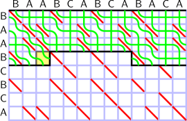
Example 7.3.
Figure 7.1 shows a snapshot of Algorithm 7.2, using the same conventions as Figure 5.1. The seaweed braid is laid out on a period subdag ; each seaweed leaving the subdag on the right is replaced by a seaweed from the same periodic family entering the subdag at the corresponding point on the left. Note that, although the two seaweeds meeting in the highlighted current cell do not cross in the current period subdag, they have both arrived from the previous period subdag, where they did cross. Therefore, their crossing has been undone in the current cell. ■
7.2 Tandem alignment
The periodic LCS problem has many variations that can be solved by an application of wraparound seaweed combing (Algorithm 7.2).
Tandem LCS.
The first such variation is the tandem LCS problem. The problem asks for the LCS score of a string of length against a tandem -repeat string of length . As before, we assume that every character of occurs in at least once; we may also assume that .
The tandem LCS problem can be solved naively by considering the LCS problem directly on strings and , ignoring the periodic structure of string . The standard dynamic programming LCS algorithm [141, 175] solves the problem in time . This running time can be slightly improved by the micro-block speedup.
The tandem LCS problem can also be regarded as a special case of the common-substring LCS problem [124, 57] (see Section 5.4). Using this technique, the problem can be solved in time . The techniques of Landau et al. [57, 121] give an algorithm for the tandem LCS problem, parameterised by the LCS score of the input strings; however, the worst-case running time of this algorithm is still . Landau [120] asked if the running time for the tandem LCS problem can be improved to .
We now give an algorithm that improves on the current algorithms in time and functionality, and even exceeds Landau’s expectation. First, we call Algorithm 7.2 on strings and . Then, we count the number of nonzeros -dominated by point , i.e. nonzeros in the submatrix . Given the (say) row-period submatrix , this can be done by a sweep of its nonzeros, counting every nonzero with appropriate multiplicity. More precisely, every nonzero , , , is counted with multiplicity , if , and is skipped (counted with multiplicity ) otherwise. The solution to the tandem LCS problem is then obtained by Theorem 4.10. The overall running time is dominated by the call of Algorithm 7.2, which runs in time .
Tandem alignment.
Another set of variations on the periodic LCS problem was introduced by Benson [24] as the tandem alignment problem. Instead of asking for all string-substring LCS scores of against , the tandem alignment problem asks for a substring of that is closest to in terms of alignment score (or edit distance), under different restrictions on the substring. In particular:
-
the pattern global, text global (PGTG) tandem alignment problem restricts the substring of to consist of a whole number of copies of , i.e. to be of the form for an arbitrary integer ;
-
the tandem cyclic alignment problem restricts the substring of to be of length for an arbitrary integer (but it may not consist of a whole number of copies of );
-
the pattern local, text global (PLTG) tandem alignment problem leaves the substring of unrestricted.
All these three versions of the tandem alignment problem can be regarded as special cases of the approximate pattern matching problem (see Section 6.2) on strings of length and of length (but with the roles of the text and the pattern reversed with respect to Benson’s terminology). Therefore, the tandem LCS problem can be solved naively by considering the approximate pattern matching problem directly on strings and , ignoring the periodic structure of string . Given an arbitrary (real) set of alignment weights, the standard dynamic programming algorithm [159] solves the problem in time . For a rational set of weights, the running time can be slightly improved by the micro-block speedup (see Section 6.2).
The PGTG and PLTG tandem alignment problems can be solved more efficiently by the technique of wraparound dynamic programming [137, 77] (see also [24]) in time . For the tandem cyclic alignment problem, Benson [24] modified this technique to give an algorithm running in time .
We now give a new algorithm for the tandem cyclic alignment problem, which improves on the existing algorithm in running time, assuming a rational set of alignment weights. The running time of the new algorithm matches the current algorithms for the PGTG and PLTG tandem alignment problems.
Given input strings , , we first solve the periodic string-substring problem by calling Algorithm 7.2. This gives us a period submatrix of matrix , where . Then, for each , , we perform independently the following procedure. We solve the tandem LCS problem for strings and by the method described earlier in this section, counting every nonzero in the period submatrix with an appropriate multiplicity. This gives us the LCS score for against for every . We then update this score incrementally, obtaining the LCS score for string against a window of length in , sliding through successive positions. This is equivalent to querying successive elements in a diagonal of matrix , which can be achieved by incremental dominance counting queries. By Theorem 2.17, every one of these queries can be performed in time .
The call to Algorithm 7.2 runs in time ; its output is shared by the tandem LCS computation for all . For each , the running time of the remaining computation is . Therefore, the combined running time for all values of is . Overall, the algorithm runs in time .
Chapter 8 Permutation string comparison
In this chapter, we consider the semi-local comparison of permutation strings.
This chapter is organised as follows. In Section 8.1, we introduce the semi-local LCS problem on permutation strings, and develop an algorithm for its solution. By direct application of this algorithm, in Section 8.2 we obtain an improved algorithm for the cyclic LCS problem on permutations. Further applications include improved algorithms for the longest pattern-avoiding subsequence problem, given in Section 8.3, and for the longest -increasing and -modal subsequence problems, given in Section 8.4. In Section 8.5, we consider the maximum clique problem in a circle graph represented by an interval model. By application our semi-local LCS algorithm on permutations, we obtain new algorithms for this problem, both for general and sparse circle graphs, achieving a substantial improvement on existing algorithms in running time. In Section 8.6, we describe an application of these algorithms to the problem of finding exact and approximate commonly structured patterns in linear graphs.
8.1 Semi-local LCS between permutations
An important special case of string comparison is where each of the input strings , is a permutation string, i.e. a string that consists of all distinct characters. Without loss of generality, we may assume that , and that both strings are permutations of a given totally ordered alphabet of size . For consistency with the notation in previous chapters, we will assume that a permutation string of length is indexed by half-integers , and is over the alphabet , unless indicated otherwise. The identity permutation string of length is the string .
Given a string , we denote its reverse string by . In particular, the reverse identity permutation string is . We denote by the set of characters appearing in at least once.
The LCS problem on permutation strings is closely related to the following classical problem.
Definition 8.1.
Given a string , the longest increasing subsequence (LIS) problem asks for the length of the longest string that is an increasing subsequence of . For consistency with our previous terminology, we will call this length the LIS score of string . □
Indeed, the LIS problem is equivalent to the LCS problem on string against the identity string , and the LCS problem on a pair of permutation strings can be reduced to the LIS problem by sorting one of the input strings.
The LIS problem has a long history, going back to Erdös and Szekeres [72] and Robinson [152]. Later, Knuth [115], Fredman [79] and Dijkstra [69] gave algorithms running in time . The problem was studied further by Chang and Wang [46], Bespamyatnikh and Segal [27]. Crochemore and Porat [60] gave an LIS algorithm running in time , where is the output LIS score.
We consider the semi-local LCS problem on permutation strings. Note that its string-substring component is equivalent to the local LIS problem, which asks for the LIS score in every substring of a given permutation string. We now give an efficient algorithm for the semi-local LCS problem on permutation strings.
Algorithm 8.2.
(Semi-local LCS between permutation strings: Seaweed doubling)
permutation strings , of length over an alphabet of size .
nonzeros of the semi-local seaweed matrix .
Recursion on .
The computation is trivial.
Assume without loss of generality that is even. We partition the input string into a concatenation of two strings of length . Each of the strings , is a permutation string over an alphabet of size .
The semi-local seaweed matrices , , are each over , and each contain nonzeros. The semi-local seaweed matrix is over , and contains nonzeros.
Note that whenever (respectively ), we have (respectively, ), so the corresponding set of indices defines within (respectively, ) an non-contiguous submatrix equal to the identity matrix .
Let be a -subsequence of , obtained by deleting all characters not belonging to . We call the algorithm recursively on strings , to compute the semi-local seaweed matrix . Then, matrix is obtained by inserting a set of rows and columns into matrix , which corresponds to reinserting the deleted characters of string into string . The newly inserted rows and columns are filled with (implicit) zeros and ones, so that they form a non-contiguous submatrix equal to the identity matrix .
Symmetrically, matrix is obtained by deleting from string all characters not belonging to , calling the algorithm recursively, and then inserting a set of rows and columns into resulting matrix to form a non-contiguous identity submatrix.
Given matrices , , the output matrix is computed by the algorithm of Theorem 4.21, which calls the algorithm of Theorem 3.16 as a subroutine. Note that we now have two nested recursions: the outer recursion of the current algorithm, and the inner recursion of Theorem 3.16.
The recursion tree is a balanced binary tree of height . In the root node, the running time is dominated by the call to the algorithm of Theorem 4.21, and is therefore . In each subsequent level of the recursion tree, the number of nodes doubles, and the running time per node is reduced by at least a factor of . Therefore, the running time per level is . The overall running time is . ■
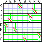
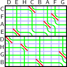
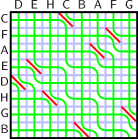
Example 8.3.
By keeping the algorithm’s intermediate data, we obtain a data structure that allows efficient traceback of any semi-local LCS query on a pair of permutations, in time proportional to the size of the output (i.e. the length of the output subsequence).
8.2 Window and cyclic LIS
Recall from Section 5.5 that, given a fixed parameter , we call a substring of length a -window in the corresponding string. The window LCS problem between permutation strings is equivalent to the window LIS problem, which asks for the LIS score in every -window of a given permutation string.
The window LIS problem has been studied by Albert et al. [9] and by Chen et al. [49]. In particular, work [49] gives an algorithm that reports all window LIS (as opposed to just their lengths) in time . In the same work, the algorithm is also generalised for reporting all LIS in an arbitrary subset of substrings of the input permutation string, possibly of different sizes. Deorowicz [68] considered the problem of finding, for a given , the maximum LIS score across all -windows of the input string. The resulting algorithm runs in time , where is the output maximum LIS score. In all the above versions of the problem, the length of each window LCS can be as high as , and therefore the algorithms’ running time can be as high as .
Using our techniques, the window LIS problem on a permutation string of size can be solved as follows. Consider a subset of -windows in , overlapping over prefixes and suffixes of length : , , , …First, we run Algorithm 8.2 (seaweed doubling) on each of these -windows against the identity permutation string , obtaining the semi-local seaweed matrix . Then, we perform string-substring LCS score queries for every -window of against . This can be done efficiently as a diagonal batch query via Theorem 2.17. Every -window of is a substring in some string among the considered subset of overlapping -windows, hence we have obtained the full solution to the window LIS problem. The overall running time is dominated by the calls to Algorithm 8.2, which run in combined time .
The cyclic LCS problem has been defined in Section 5.5. The cyclic LCS problem on a pair of permutation strings is equivalent to the cyclic LIS problem, which asks for the maximum LIS score across all cyclic shifts of the input string.
The cyclic LIS problem has been considered by Albert et al. [8], who gave a Monte Carlo randomised algorithm, running in time with small error probability. Deorowicz [67] observed that [8] also provides a deterministic algorithm for cyclic LIS, running in time , and gave an improved algorithm running in time .
We now give a simple algorithm for the cyclic LIS problem, similar to the cyclic LCS algorithm given in Section 5.5, but based on the semi-local LCS problem for permutation strings. First, we run Algorithm 8.2 (semi-local LCS between permutation strings), obtaining the semi-local seaweed matrix . Then, we run the algorithm of Theorem 4.21 on matrix against itself, obtaining the semi-local seaweed matrix . Finally, we perform substring-string LCS queries for every substring of of length against string . The overall running time is dominated by the call to Algorithm 8.2, which runs in time .
The resulting algorithm for the cyclic LIS problem improves on existing algorithms both in running time, and by being deterministic. In particular, our algorithm is faster than the algorithm of [67], unless .
8.3 Longest pattern-avoiding subsequences
Two given permutation strings , of equal length (but generally over different alphabets) are called isomorphic, if they have the same relative order of characters, i.e. iff for all , . Given a target permutation string of length and a pattern permutation string of fixed length, the longest -isomorphic subsequence problem, or simply the longest -subsequence problem, asks for the longest subsequence of that is isomorphic to . More generally, given a set of pattern permutation strings , the longest -subsequence problem asks for the longest subsequence of that is isomorphic to any pattern string in .
Example 8.4.
The LIS problem can be interpreted as the longest -subsequence problem, where . ■
Given a set of antipattern permutation strings , the longest -avoiding subsequence problem asks for the longest subsequence of that does not contain a subsequence isomorphic to any string in .
Example 8.5.
The LIS problem on a permutation string can be interpreted as the longest -avoiding subsequence problem. ■
For a detailed introduction into these problems and their connections, see the work by Albert et al. [7] and references therein.
The LIS problem is the only nontrivial example of the longest -avoiding subsequence problem with antipatterns of length . Albert et al. [7] gave the full classification of the longest -avoiding subsequence problem for all sets of antipatterns of length . There are 10 non-trivial sets of such antipatterns. For each of these sets, the algorithms given in [7] run in polynomial time, ranging from to . Two particular antipattern sets considered in [7] are (in that work’s original notation):
For both these antipattern sets, algorithms given in [7] run in time .
We now give new algorithms for the longest - and -avoiding subsequence problems, improving on the above algorithms in running time.
Permutation strings that are -avoiding are all cyclic rotations of an increasing permutation string. The longest such subsequence in the target string can be found by the algorithm for the cyclic LCS problem between permutations (Section 8.2), running in time .
Permutation strings that are -avoiding are all obtained from an increasing permutation string by reversing some suffix. The longest -avoiding subsequence in the target string can be found as follows. Let the target string be over the alphabet . First, we call the standard LIS algorithm on , obtaining explicitly the prefix-prefix LCS scores
for all . Independently, we call the seaweed doubling algorithm (Algorithm 8.2) on against the reverse identity permutation , and use Theorem 2.15 to process its output into a data structure that allows efficient queries of all suffix-prefix LCS scores for all . Finally, we obtain the solution to the longest -avoiding subsequence problem as
The overall running time is dominated by the call to Algorithm 8.2, which runs in time .
8.4 Longest piecewise monotone subsequences
The classical LIS problem asks for the longest increasing (or, equivalently, decreasing) subsequence in a permutation string. A natural generalisation is to ask for the longest subsequence that consists of a constant number of monotone pieces. In particular, given a permutation string of length , the longest -increasing subsequence (respectively, longest -modal subsequence) problem asks for the longest subsequence in that is a concatenation of at most sequences, all of which are increasing (respectively, alternate between increasing and decreasing). In the case of the longest -modal subsequence problem, we assume without loss of generality that is even. Both problems can be solved as an instance of the LCS problem, comparing the input permutation string against string , i.e. the concatenation of copies of the identity permutation (respectively, against string , i.e. the concatenation of alternating copies of and its reverse ). The resulting alignment dag is of size , and contains match cells. Using standard sparse LCS algorithms [99, 17], such an instance of the LCS problem can be solved in time . Demange et al. [64] gave a similar algorithm for the longest -modal subsequence problem, also running in time .
We now give new algorithms for the longest -increasing subsequence and the longest -modal subsequence problems, improving on the above algorithms in running time for sufficiently large .
To solve the longest -increasing subsequence problem, we run Algorithm 8.2 (seaweed doubling), obtaining the semi-local seaweed matrix , from which we extract the string-substring seaweed matrix . We then run the algorithm of Theorem 4.21 repeatedly times, obtaining the string-substring seaweed matrix .
For the the longest -modal subsequence problem, assume without loss of generality that is even. To solve this problem, we first run Algorithm 8.2 (seaweed doubling) twice, on strings and , respectively, against string . As as a result, we obtain the semi-local seaweed matrices and . We then obtain matrix by Theorem 4.21. From this matrix, we extract the string-substring seaweed matrix . We then run the algorithm of Theorem 4.21 repeatedly times, obtaining the string-substring seaweed matrix .
The final step of the algorithm is identical for both problems: we use the obtained string-substring seaweed matrix ( and , respectively) to query the global LCS score. Both described algorithms run in time . This is faster than both the sparse LCS approach and the algorithm of [64], for all .
8.5 Maximum clique in a circle graph
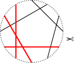
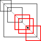
A circle graph [74, 87] is defined as the intersection graph of a set of chords in a circle, i.e. the graph where each node represents a chord, and two nodes are adjacent, whenever the corresponding chords intersect. We consider the maximum clique problem on a circle graph.
The interval model of a circle graph is obtained by cutting the circle at an arbitrary point and laying it out on a line, so that the chords become (closed) intervals. The original circle graph is isomorphic to the overlap graph of its interval model, i.e. the graph where each node represents an interval, and two nodes are adjacent, whenever the corresponding intervals intersect but do not contain one another.
Example 8.6.
Figure 8.2 shows an instance of the maximum clique problem on a six-node circle graph. Subfigure 8.2a shows the set of chords defining a circle graph, with one of the maximum cliques highlighted in bold red. The cut point is shown by scissors. Subfigure 8.2b shows the corresponding interval model; the dotted diagonal line contains the intervals, each defined by the diagonal of a square. The squares corresponding to the maximum clique are highlighted in bold red. ■
It has long been known that the maximum clique problem in a circle graph on nodes is solvable in polynomial time [81]. A number of algorithms have been proposed for this problem [154, 97, 133, 14]; the problem has also been studied in the context of line arrangements in the hyperbolic plane [109, 71]. Given an interval model of a circle graph, the running time of the above algorithms is in the worst case, i.e. when the input graph is dense. In [164, 166], we gave an algorithm running in time .
We now give a new algorithm for the maximum clique problem in a circle graph, improving on existing algorithms in running time. The algorithm is based on the fast implicit distance multiplication procedure of Theorem 3.16.
Our algorithm takes as input the interval model of a circle graph on nodes. Without loss of generality, we may assume that the set of interval endpoints is . The interval model is represented by a permutation string of size , where for each left (respectively, right) interval endpoint , is the corresponding right (respectively, left) endpoint. Note that for all , an interval with left endpoint does not contain an interval with left endpoint , if and only if . Various alternative representations of interval models (e.g. the ones used in [154, 14]) can be converted to this representation in linear time.
In the interval model, a clique corresponds to a set of pairwise intersecting intervals, none of which contains another interval from the set. Recall that intervals in the line satisfy the Helly property: if all intervals in a set intersect pairwise, then they all intersect at a common point. In our context, we only need to consider integer indices as intersection points.
Consider a clique in . Let be a common intersection point of the intervals representing the clique, which is guaranteed to exist by the Helly property. Since the intervals representing the clique cannot contain one another, the sequence of their right endpoints is an increasing subsequence of . Let be the identity permutation string of length . From the observations above, it follows that the clique corresponds to a common subsequence of a prefix and a suffix . Therefore, the maximum clique problem can be solved as an instance of the semi-local LCS problem.
Algorithm 8.7.
(Maximum clique in a circle graph)
interval model of circle graph , represented by permutation string of size .
maximum-size clique of , represented by the corresponding set of intervals.
We run Algorithm 8.2 on the input permutation string against the identity permutation string , obtaining the seaweed matrix . We then build the data structure of Theorem 2.15 for querying semi-local LCS scores of against .
The size of the maximum clique can now be obtained as
For each , the prefix-suffix LCS score is queried from seaweed matrix by Theorem 2.15. The value for which the maximum score is attained gives a common intersection point of the clique intervals.
Let be a subsequence of the prefix , obtained by deleting all characters not belonging to the interval . The intervals defining the maximum clique can now be obtained by running a standard LIS algorithm on string , and then tracing back the elements of the resulting LIS.
The running time of Algorithm 8.2 is .
By Theorem 2.15, the combined running time of all the prefix-suffix queries is , if the queries are performed independently. This time can be reduced to by observing that the queries can be performed as a single diagonal batch query of the type described by Theorem 2.15.
The LIS algorithm on string runs in time .
The overall running time is . ■
Like many algorithmic problems, the problem of finding a maximum clique in a circle graph admits various parameterised versions. Some relevant parameters are:
-
the size of the maximum clique;
-
the thickness of the interval model, i.e. the maximum number of intervals containing a point, taken across all points in the line;
-
the number of graph edges.
For any interval model of a non-trivial circle graph, we have . Notice that, given a permutation representing an interval model, its thickness can be found in time by building a range tree on the corresponding set of planar points, and then performing dominance counting queries.
Apostolico et al. [14] give algorithms for the parameterised version of the maximum clique problem in a circle graph, running in time and . They also describe an algorithm for the maximum independent set problem, parameterised by the interval model’s thickness.
We now give a new algorithm for the maximum clique problem in a circle graph, parameterised by the thickness of the input interval model. Our algorithm improves on the parameterised algorithms of [14] for most values of the parameters. The algorithm is an extended version of Algorithm 8.7.
Algorithm 8.8.
(Maximum clique in a circle graph, parameterised by thickness)
interval model of circle graph , represented by string of size .
maximum-size clique of , represented by the corresponding set of intervals.
thickness , , of the input interval model.
We run Algorithm 8.2 on string against string , independently for all . As will be shown in the algorithm’s analysis, in each run we obtain a seaweed matrix with at most non-trivial nonzeros. For every , we then build the data structure of Theorem 2.15 for querying semi-local LCS scores of against .
The size of the maximum clique can now be obtained as
For each , the prefix-suffix LCS score is queried from seaweed matrix by Theorem 2.15. The value for which the maximum score is attained gives a common intersection point of the clique intervals.
As in Algorithm 8.7.
Consider the string decomposition
The alignment dag is therefore the composite of alignment dags and .
The alignment dag contains at most match cells, since every match corresponds to an interval containing point , and there can be at most such intervals by the definition of thickness. The alignment dag also contains at most match cells, since the length of the string is . Hence, the alignment dag contains at most matches. Therefore, the time for each run of Algorithm 8.2 is , and the overall running time of this phase is .
By Theorem 2.15, the combined running time of all the prefix-suffix queries is , if the queries are performed independently. This time can be reduced to by observing that the queries can be performed as a set of diagonal batch queries of the type described by Theorem 2.15.
String contains at most characters, since every such character corresponds to an interval containing point . Therefore, the LIS algorithm on string runs in time .
The overall running time is . ■
8.6 Maximum common pattern between linear graphs
The concept of a linear graph, introduced by Davydov and Batzoglou [63], is similar to an interval model of a circle graph defined in Section 8.5. The interval relations of disjointness, containment and overlapping are denoted respectively by symbols , and . A pattern in a linear graph is defined as an ordered subset of intervals, all of which satisfy pairwise a prescribed subset of relations.
Fertin et al. [76] considered the maximum common -structured pattern (-MCSP) problem. The problem asks for the maximum common pattern in a set of linear graphs, each defined by at most intervals, where the structure of the common pattern is restricted by a prescribed subset of relations . In particular, the -MCSP problem asks for the maximum commonly-structured subset of pairwise overlapping intervals; for this is equivalent to finding the maximum clique of a circle graph, and for general is equivalent to finding the minimum-sized clique among maximum cliques of the input circle graphs. The -MCSP problem asks for the maximum commonly-structured subset of intervals, no two of which are overlapping; for this is equivalent to finding the maximum independent set of a circle graph; however, for general the maximum commonly-structured independent set of the input circle graphs may be significantly different from (and smaller than) each of the individual maximum independent sets. The -MCSP problem asks for the maximum commonly-structured subset of intervals without any a priori restriction on its structure.
Extending and generalising a number of previous results, paper [76] considers the -MCSP problem, where runs over all seven nonempty subsets of . For some of these seven variants, the algorithms use as a subroutine the algorithm of [164, 166] for the maximum clique problem in a circle graph. By plugging in the more efficient Algorithm 8.7, we can obtain improved algorithms for those variants of the -MCSP problem, where finding the maximum clique in a circle graph is a bottleneck.
In particular, the -MCSP problem is solved in [76] by finding the maximum clique independently for circle graphs, each corresponding to one of the input linear graphs, in overall time . By plugging in Algorithm 8.7, the running time is improved to .
The -MCSP problem is shown in [76] to be NP-hard, and to admit a polynomial-time -approximation, where ; for the rest of this section, denotes the size of the optimal solution to the problem. The approximation is obtained by calls to the following subroutine: given a circle graph of size , and two integers , , decide whether the graph contains disjoint cliques, each of size . This subroutine is performed in time , and therefore the overall running time is . By a straightforward extension of Algorithm 8.7, the running time of the subroutine is improved to , and therefore the overall running time of the approximation algorithm is improved to .
The -MCSP problem is also shown in [76] to be NP-hard, and to admit a polynomial-time -approximation. The approximation is obtained by combining exact solutions for the -MCSP and -MCSP problems on the same input sets. The exact solution for the -MCSP is the bottleneck; by plugging in the improved algorithm for this problem described above, the running time of the approximation algorithm for the -MCSP problem is improved from to .
Finally, paper [76] argues that the -MCSP problem is NP-hard, and gives several polynomial-time approximation algorithms. In particular, it gives an -approximation algorithm running in time , and an -approximation algorithm running in time . By using the techniques described above, the running times of these approximation algorithms are improved respectively to and .
Chapter 9 Compressed string comparison
In this chapter, we consider the semi-local comparison of compressed strings.
This chapter is organised as follows. In Section 9.1, we introduce the grammar compression (GC) framework, that generalises the classical LZ78 and LZW methods. In Section 9.2, we describe a folklore algorithm for global subsequence recognition in a GC-string. In Section 9.3, we develop an efficient algorithm for the extended substring-string problem between a plain pattern and a GC-string. By application of this algorithm, in Section 9.4 we obtain an algorithm for local subsequence recognition in a GC-string, and in Section 9.5 an algorithm for threshold approximate matching in a GC-string; both these algorithms improve on the existing ones in running time.
9.1 Grammar-compressed strings
String compression is a classical paradigm, touching on many different areas of computer science. From an algorithmic viewpoint, it is natural to ask whether compressed strings can be processed efficiently without decompression. Early examples of such algorithms were given e.g. by Amir et al. [12] and by Rytter [155]; for a recent survey on the topic, see Lohrey [128]. Efficient algorithms for compressed strings can also be applied to achieve speedup over ordinary string processing algorithms for plain strings that are highly compressible.
We consider the following general model of compression.
Definition 9.1.
Let be a string of length (typically large). String will be called a grammar-compressed string (GC-string), if it is generated by a context-free grammar, also called a straight-line program (SLP). An SLP of length , , is a sequence of statements. A statement numbered , , has one of the following forms:
where is an alphabet character, and each of , is either an alphabet character, or symbol for some , . □
We identify every symbol with the string it expands to; in particular, we have . In general, the plain string length can be exponential in the GC-string length .
Example 9.2.
The Fibonacci string “ABAABABAABAAB” of length 13 can be represented by the following SLP of length 6:
In general, a Fibonacci string of length can be represented by an SLP of length , where is the -th Fibonacci number.
This example is borrowed from Hermelin et al. [93]. ■
Kida et al. [112] introduced a more general compression model, called collage systems. Grammar compression is a equivalent to a subclass of collage systems called regular. As a special case, grammar compression includes the classical LZ78 and LZW compression schemes by Ziv, Lempel and Welch [181, 176]. Both these schemes can be expressed by an SLP that consists of three sections:
-
in the first section, all statements are of the form ;
-
in the second section, all statements are of the form , where statement is from the first section;
-
in the third section, all statements are of the form , where statement is from the second section.
It should also be noted that certain other compression methods, such as e.g. LZ77 [180] and run-length compression, do not fit directly into the grammar compression model.
The algorithms in this section will take as input a plain (uncompressed) pattern string of length , and a grammar-compressed text string of length , generated by an SLP of length . We aim at algorithms with running time that is a low-degree polynomial in , , but is independent of (which could be exponential in ).
9.2 Global subsequence recognition
The first problem that we consider on a compressed text is the global subsequence recognition problem, introduced in Section 4.1. Recall that on a plain text, this problem can be solved in time by a straightforward algorithm. We now revisit this problem, assuming a plain pattern and a GC-text as inputs. We also generalise the problem slightly, looking for the length of the longest prefix of that is a subsequence of . The problem can be solved by a simple folklore algorithm as follows.
Algorithm 9.3 (Global subsequence recognition).
plain pattern string of length ; SLP of length , generating text string of length .
an integer , giving the length of the longest prefix of that is a subsequence of . String contains as a subsequence, if and only if .
Recursion on the input SLP generating .
The output value is determined by a single character comparison.
Let be the SLP statement defining string . Let be the length of the longest prefix of that is a subsequence of . Let be the length of the longest prefix of that is a subsequence of . We call the algorithm recursively to obtain and , and then return .
The running time of the algorithm is . The proof is by induction. The running time of the recursive calls is respectively and . The overall running time of the algorithm is . In the worst case, this is . ■
9.3 Extended substring-string LCS
We now consider the LCS problem. Recall from Sections 4.1, 5.2 that on a pair of plain strings, it can be solved in time , assuming that . The LCS problem on two GC-strings has been considered by Lifshits and Lohrey [127, 128], and proven to be PP-hard (and therefore NP-hard).
In this section, we revisit the LCS problem, now assuming a plain pattern and a GC-text as inputs. Although, in principle, we would like to solve the more general semi-local LCS problem, it would be impossible to do so while keeping the running time independent of , since the resulting semi-local seaweed matrix would require memory . However, we are still able to solve the extended substring-string LCS problem (i.e. string-substring, prefix-suffix and suffix-prefix LCS), where the output only requires memory .
In the special case of LZ77 or LZW compression of the text, the algorithm of Crochemore et al. [58] solves the LCS problem in time . Thus, LZ77 or LZW compression of one of the input strings only slows down the LCS computation by a constant factor relative to the classical dynamic programming LCS algorithm, or by a polylogarithmic factor relative to the best known LCS algorithms.
The general case of an arbitrary GC-text appears more difficult. A GC-text is a special case of a context-free language, which consists of a single string. Therefore, the LCS problem between a GC-text and a plain pattern can be regarded as a special case of the edit distance problem between a context-free language given by a grammar of size , and a pattern string of size . For this more general problem, Myers [138] gave an algorithm running in time . In [167], we gave an algorithm for the three-way semi-local LCS problem between a GC-text and a plain pattern, running in time . Lifshits [126] asked whether the LCS problem in the same setting can be solved in time .
A new algorithm for the extended substring-string LCS problem can be obtained by an application of the techniques described in Chapter 4. The resulting algorithm improves on existing algorithms in running time, and approaches an answer to Lifshits’ question within a logarithmic factor.
Algorithm 9.4 (Extended substring-string LCS).
plain pattern of length ; SLP of length , generating text of length .
nonzeros of matrix .
First, we observe that, although the output matrix contains at most nonzeros, its range is of size , which may be exponentially larger. To avoid an exponential growth of the indices, we will clean up the range by removing unused indices, and deleting the corresponding zero row-column pairs from the matrix. Formally, we describe this process as an order-preserving remapping of the index range.
Recursion on the input SLP generating .
The output can be computed by Algorithm 5.1 (seaweed combing) on plain strings and , of length and respectively.
Let be the SLP statement defining string . We call the algorithm recursively to obtain the nonzeros of matrices , . The total number of nonzeros in each matrix is between and . Conceptually, the ranges of these matrices are respectively , and . However, the actual remapped range for each matrix is after the respective recursive call.
We now compute the matrix from , by Theorem 4.21. The total number of nonzeros in this matrix is again between and . Conceptually, the range of this matrix is . However, the actual remapped index range after the application of Theorem 4.21 is . Therefore, there are at least indices , such that the row and the column both contain only zeros. We now delete exactly such rows and columns from the matrix, and remap the index range to , while preserving the linear order of the indices.
We now have the nonzeros of the output matrix , remapped to the range . This is already sufficient to query the global LCS score, or extended substring-string LCS scores for pattern against text . However, if explicit indices of the nonzeros in the output matrix are required, the index range can be remapped back to by reversing every remapping step in the first phase.
The cost of a recursive step is dominated by the application of Theorem 4.21, which runs in time . There are recursive steps in total, therefore the first phase runs in time .
For each nonzero, the inverse remapping can be performed recursively in time . There are nonzeros in total, therefore the second phase runs in time .
The overall running time is . ■
Algorithm 9.4 provides, as a special case, an algorithm for the LCS problem between a plain string and a GC-string, running in time ; the LCS score can easily be queried from the algorithm’s output matrix by Theorem 4.10. This running time should be contrasted with standard LCS algorithms on plain strings, running in time [132, 58], and with the PP-hardness of the LCS problem on two GC-strings [127, 128].
Hermelin et al. [93] and Gawrychowski [82] refined the application of our techniques as follows. They consider the rational-weighted alignment problem (equivalently, the LCS or Levenshtein distance problems) on a pair of GC-strings , of total compressed length , parameterised by the strings’ total plain length . The algorithm of [93] runs in time , which is improved in [82] to . In both cases, our algorithm of Theorem 3.16 is used as a subroutine.
9.4 Local subsequence recognition
The local subsequence recognition problem was introduced in Section 4.2 as a special case of the semi-local LCS problem, and defined in Section 6.2 (Definition 6.14) as a variant of the approximate matching problem. In the context of local subsequence recognition, a substring of text is called a matching substring, if it contains the pattern as a subsequence. A matching substring will be called minimally matching, if it is inclusion-minimal, i.e. it has no proper matching substring.
We recall that, depending on the output filtering, local subsequence recognition can take the following forms: the minimum-window subsequence recognition problem, which asks for the locations of all substrings of that are minimally matching, and the fixed-window subsequence recognition problem, which asks for the locations of all the matching substrings of a fixed length . A combination of these two problems is the bounded minimal-window subsequence recognition problem, which asks for the locations of all the minimally matching substrings below a fixed length .
Clearly, the output size for the described reporting versions of these problems may be exponential in ; therefore, we have to parameterise the running time by the output size, which we denote by . We will also consider the counting version for each of the above problems, which, instead of locations of all the matching substrings, only asks for their overall number. The running time of the counting algorithms described in this section will be the running time of the corresponding reporting algorithm with .
The minimal-window, fixed-window and bounded minimal-window subsequence recognition problems for a GC-text against a plain pattern have been considered by Cégielski et al. [42]. For each problem, they gave an algorithm running in time . In [167], we gave an algorithm improving the running time for these problems to , and then in [170] improved it to by an extended version of Algorithm 9.4. Yamamoto et al. [179], using elementary techniques, gave an even faster algorithm, running in time .
We now describe the algorithm of [170] for local subsequence recognition. Although inferior, both in running time and simplicity, to the algorithm of [179], it will serve as a warm-up for the material presented in the next section.
We extend Algorithm 9.4 (extended string-substring LCS) as follows. In addition to the extended substring-string matrix , we now also make use of the cross-semi-local matrix . This matrix is used for reporting the minimally matching substrings that are cross-substrings in the current recursive step.
Algorithm 9.5 (Local subsequence recognition).
plain pattern of length ; SLP of length , generating text of length .
locations (or count) of minimally matching substrings in .
Similarly to Algorithm 9.4, index remapping has to be performed in the background in order to avoid an exponential growth of the indices. To simplify the exposition, we now assume constant-time index arithmetic, keeping the index remapping implicit.
Recursion on the input SLP generating .
As in Algorithm 9.4, the extended substring-string matrix can be computed by Algorithm 5.1 (seaweed combing) on plain strings and , of length and respectively. String is matching, if and only if and ; in this case, is also minimally matching.
Let be the SLP statement defining string . We run a recursive step of Algorithm 9.4, obtaining the extended substring-string seaweed matrix . In addition, we obtain the cross-semi-local seaweed matrix by Theorem 4.21.
As in Algorithm 9.5, we run a recursive step of Algorithm 9.4, obtaining the extended substring-string seaweed matrix . In addition, we obtain the cross-semi-local seaweed matrix by Theorem 4.21. These two subpermutation matrices are typically very sparse: their index range is of size , where is typically much higher than , whereas the number of nonzeros in either matrix is at most (for matrix , it is exactly ).
By Theorem 4.10, a substring is matching, if and only if , i.e. the point in the score matrix is not -dominated by any nonzeros in the seaweed matrix . Recall that a substring is a cross-substring, if , ; in other words, a cross-substring consists of a non-empty suffix of and a non-empty prefix of . A point corresponding to a cross-substring lies within the cross-semi-local score matrix , and can only be -dominated by one of the nonzeros in the cross-semi-local seaweed matrix .
Let
be the -chain of all -maximal nonzeros in , where . If a point is -dominated by any nonzeros in , then it is dominated by some -maximal nonzero, i.e. by a point in . Therefore, a cross-substring is matching, if and only if point is not -dominated by any point in .
Consider the set of all points in that are not -dominated by any point in . We are interested in the -minimal points in this set. Such points form a -chain, interleaved with . Its two endpoints are the degenerate boundary points , ; the remaining points form a -chain of size :
Let be the subset of points in within the string-cross-substring score matrix . A non-degenerate cross-substring is minimally matching, if and only if . The number of such cross-substrings is .
For every SLP symbol, we now have the relative locations of its minimally matching cross-substrings. Furthermore, every non-trivial substring of corresponds to a cross-substring for some SLP symbol, under an appropriate transformation of indices. By another recursion on the structure of the SLP, it is now straightforward to obtain either the absolute locations, or the count of all the minimally matching substrings in .
As in Algorithm 9.4, each seaweed matrix multiplication runs in time . The -chains and can be obtained in time . Hence, the running time of a recursive step is . There are recursive steps in total, therefore the whole recursion runs in time .
For every SLP symbol, there are at most minimally matching cross-substrings. Given the output of the first phase, the absolute locations of all minimally matching substrings in can be reported in time , and their count can be obtained in time .
The overall running time is for reporting, and for counting. ■
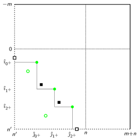
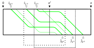
Example 9.6.
Figure 9.1 shows a snapshot of a recursive step in the first phase of Algorithm 9.5. Subfigure 9.1a shows the cross-semi-local matrices and ; in this particular example, all the nonzeros of the latter lie within the string-cross-substring matrix . Subfigure 9.1b shows the corresponding seaweed braid. Matrix contains nonzeros, shown by green circles in Subfigure 9.1a, and by green seaweeds in Subfigure 9.1b. Out of these five nonzeros, three are -maximal. These nonzeros form the -chain ; they are shown by filled circles connected by a thin zig-zag line in Subfigure 9.1a, and by thicker seaweeds in Subfigure 9.1b. The remaining two nonzeros are shown by hollow circles (respectively, by thinner seaweeds). All points in that are not -dominated by any nonzeros in are located above and to the right of the thin zig-zag line. The four -minimal such points are shown in Subfigure 9.1a by black squares; among these, two are degenerate boundary points (hollow squares), and the other two form the -chain (filled squares). Both points of chain lie within the range , therefore , and each of the two points in corresponds to a minimally matching non-degenerate cross-substring in . These two substrings are shown in Subfigure 9.1b by dotted brackets.
By Theorem 4.10, a substring in is matching, if and only if the corresponding rectangle in the alignment dag is not pierced by a seaweed entering at its left-hand boundary and leaving at its right-hand boundary. Notice that the bracketed substrings of in Figure 9.1b are exactly the two inclusion-minimal non-degenerate cross-substrings satisfying this property. ■
An algorithm for the fixed-window subsequence recognition problem can be obtained from Algorithm 9.5 as follows. Substrings of length correspond to points lying on the diagonal in the semi-local score matrix . Consider the set of all points on this diagonal, -dominated by any point in the -chain , introduced in Algorithm 9.5. This set consists of a (not necessarily disjoint) union of diagonal intervals
where any interval of negative length is by convention considered empty. In every recursive step, the interval endpoints in the set can be computed in time .
A cross-substring , , is matching, if and only if . Therefore, each point corresponding to a cross-substring of can be reported in constant time.
An algorithm for the bounded minimal-window subsequence recognition problem can be obtained from Algorithm 9.5 by discarding in every recursive step the minimally matching cross-substrings of length exceeding .
The overall running time of both the above modifications of Algorithm 9.5 is still .
9.5 Edit distance matching
The edit distance matching problem was introduced in Section 6.2 (Definition 6.15). In the context of edit distance matching, a substring of text will be called a matching substring, if it has alignment score at least against pattern (alternatively, edit distance at most ), where (respectively, ) is a fixed threshold.
Approximate pattern matching on compressed text has been studied by Kärkkäinen et al. [108]. For a GC-text of length , an uncompressed pattern of length , and an edit distance threshold , the (suitably generalised) algorithm of [108] solves the edit distance matching problem in time . In the special case of LZ78 or LZW compression, the running time is reduced to . Bille et al. [31] gave an efficient general scheme for adapting an arbitrary edit distance matching algorithm to work on a GC-text. The running time of the resulting algorithms is parameterised by the text’s plain length ; note that . In particular, when the algorithms by Landau and Vishkin [123] and by Cole and Hariharan [51] are each plugged into this scheme, the resulting algorithm runs respectively in time
In the special case of LZ78 or LZW compression, Bille et al. [28] show that it is possible to remove the term , reducing the running time respectively to and .
Using the techniques of the previous sections, we now show how the edit distance matching problem on a GC-text can be solved more efficiently, for a sufficiently high value of the threshold . The algorithm extends Algorithms 9.4 (extended string-substring LCS) and 9.5 (local subsequence recognition), and assumes an edit distance with arbitrary rational weights. As in Algorithm 9.5, we assume for simplicity the constant-time index arithmetic, keeping the index remapping implicit. In the algorithm’s description, it will be convenient to extend the integer and half-integer interval notation to non-integer endpoints as follows:
for any real , .
Algorithm 9.7 (Edit distance matching).
character alignment weights for a mismatch and for a gap , where . These weights are assumed to be constant rationals. The weight for a match is fixed as .
plain pattern string of length ; SLP of length , generating text string of length ; score threshold .
unique starting positions of matching substrings in .
Recursion on the input SLP generating .
To reduce the problem to an unweighted LCS score, we apply the normalisation and the blow-up techniques described in Section 6.1. Following Definition 6.6, we introduce the normalised weights , , . Let , where , are positive natural numbers. We transform strings , into the corresponding blown-up strings , of length , , respectively.
The extended substring-string seaweed matrix can be computed by Algorithm 5.1 (seaweed combing) on plain strings and , of length and respectively. This matrix can be used to query the LCS score between and . String is matching, if and only if the corresponding weighted alignment score is above the threshold: .
Let be the SLP statement defining string . We have for the corresponding blown-up strings.
As in Algorithm 9.5 (local subsequence recognition), we obtain recursively the extended substring-string seaweed matrix and the cross-semi-local seaweed matrix by Theorem 4.21. These two subpermutation matrices are typically very sparse: contains at most nonzeros, and exactly nonzeros.
Similarly to Algorithm 9.5, the matching substrings in can now be determined by the nonzeros of the cross-semi-local seaweed matrix . However, this time it is no longer sufficient to consider just its -maximal nonzeros; we now have to consider all its nonzeros. Let us denote the indices of these nonzeros, in increasing order independently for each dimension, by
| (9.1) |
These two index sequences define an non-contiguous permutation submatrix of nonzeros in :
| (9.2) |
for all .
Index sequence (respectively, ) partitions the range (respectively, ) into disjoint non-empty intervals of varying lengths:
where the boundary indices are defined as
(note that we are making use of the interval notation with non-integer endpoints). Therefore, we have a partitioning of the cross-semi-local score matrix into disjoint non-empty rectangular -blocks of varying dimensions. Consider an arbitrary -block
| (9.3) |
where . By definition of the index sequences (9.1), a nonzero of matrix can only occur at a meeting point of four different -blocks. Therefore, matrix is identically zero inside every -block: we have for all , , given any fixed index pair (again using interval notation with non-integer endpoints). Therefore, given a fixed -block, all its points are -dominated by the same set of nonzeros in matrix (and hence also in ). The number of nonzeros in this set is
| (9.4) |
where the reference point within an -block is chosen arbitrarily as its bottom-left (-minimal) point . Since the value of is constant across the -block, by Theorem 4.10 all its entries have identical value:
| (9.5) |
for all , .
We now switch our focus from the blown-up strings , , back to the original strings , , . The partitioning of the LCS score matrix into -blocks induces a partitioning of the alignment score matrix into disjoint rectangular -blocks of varying dimensions. The -block corresponding to -block (9.3) is
| (9.6) |
Note that, although an -block (9.3) is by definition non-empty, the corresponding -block (9.6) may be empty. This happens whenever either of the intervals or contains no integer points (i.e. either of the intervals or contains no multiples of ). However, for ease of notation, we will assume that all the -blocks are non-empty.
Although all entries within an -block (9.3) are constant, the entries within the corresponding -block (9.6) will typically vary. By (9.5) and Definition 6.6, we have
| (9.7) |
where , . Recall that . Therefore, the score within an -block is maximised when is minimised, so the maximum score is attained by the block’s bottom-left (i.e. -minimal) entry .
We are interested in the bottom-left entries of all the -blocks, since that is where block maxima are attained. The leftmost column and the bottom row of these entries (respectively and for all , ), lie on the bottom-left boundary of matrix ; all such boundary points are degenerate. The remaining block maxima form an non-contiguous submatrix
where , .
Let
be the submatrix of within the string-cross-substring score matrix . Since matrix is anti-Monge, its submatrices and are also anti-Monge.
We now need to obtain the row maxima of matrix . Let
| (by (9.7), (9.4), (9.2)) | |||
Since , the problem of finding row maxima of is equivalent to finding row minima of matrix , or, equivalently, column minima of the transpose matrix . This matrix (and therefore itself) is subunit-Monge: we have
where
Therefore, the column minima of can be found by either Lemma 3.12 or Lemma 3.14 (replacing row minima with column minima by symmetry).
The unique starting positions of matching non-degenerate cross-substrings in can now be obtained as indices of row maxima in scoring above the threshold .
As in Algorithm 9.5, substituting “matching” for “minimally matching”.
As in Algorithm 9.4, each seaweed matrix multiplication runs in time . The algorithms of Lemma 3.12 and Lemma 3.14 run in time and , respectively. Hence, the running time of a recursive step is . There are recursive steps in total, therefore the whole recursion runs in time .
As in Algorithm 9.5, the absolute unique matching positions of all matching substrings in can be found in time .
The overall running time is . ■
Algorithm 9.7 improves on the algorithm of [108] for in the case of general GC-compression, and in the case of LZ78 or LZW compression. Algorithm 9.7 also improves on the algorithms of [28, 31] for , in the case of both general GC-compression and LZ78 or LZW compression.
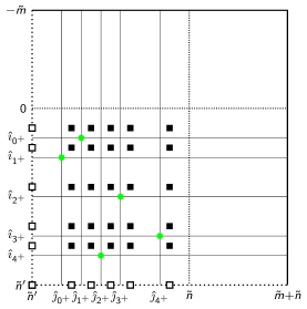
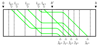
Example 9.8.
Figure 9.2 shows a snapshot of a recursive step in the first phase of Algorithm 9.7, which is assumed to run on the same input as in Figure 9.1. Subfigure 9.2a shows the cross-semi-local matrices and ; Subfigure 9.2b shows the corresponding seaweed braid. The cross-semi-local matrix and the seaweed braid are identical to the ones in Figure 9.1. In Subfigure 9.2a, submatrix and the partitioning of into -blocks is shown by a grid of thin solid lines. The bottom-left entry in each corresponding -block (note that it need not be bottom-left in the -block) is marked by a black square; among these, some are degenerate boundary points (hollow squares), and the others form submatrix . In Subfigure 9.2b, the corresponding substring boundaries are shown by dotted lines. All elements of lie within the range , therefore , and its row maxima scoring above the threshold correspond to unique starting positions of matching non-degenerate cross-substrings in . ■
Chapter 10 The transposition network method
From Chapter 4, we already know that the structure of semi-local string comparison can be expressed in two equivalent forms: the distance multiplication monoid of simple unit-Monge matrices, and the monoid of seaweed braids. In this chapter, we show that this structure can be seen in yet another alternative form, based on the classical concept of comparison networks.
10.1 Seaweed combing as a transposition network
Comparison networks were first considered as a computation model by Batcher [22] (see also [53, 6]).
Definition 10.1.
A circuit represents a computation as a dag (directed acyclic graph). The internal nodes of a circuit are labeled by elementary operations on values, which are passed along the edges; source and sink nodes represent the inputs and outputs, respectively. A comparator node (or simply comparator) is a node of indegree and outdegree 2, which sorts its two operands in increasing order. In other words, a comparator node compares the operands on the incoming edges, and returns each of the minimum and the maximum operand on a prescribed outgoing edge. A comparison network is a circuit where all internal nodes are comparator nodes. □
The most well-studied types of comparison networks are the ones that either sort their inputs, or merge two disjoint subsets of inputs. In particular, Batcher [22] gave classical merging networks with comparators, and sorting networks with comparators. Ajtai et al. [4, 5] gave an asymptotically optimal sorting network with comparators; their construction was subsequently simplified by Paterson [142] and by Seiferas [158].
Comparison networks are usually visualised by wire diagrams (also known as Knuth diagrams), where the values propagate across the network along a set of parallel wires. Every comparator is represented by a directed line segment, drawn orthogonally between two (not necessarily adjacent) wires. The order in which a comparator returns the minimum and the maximum output is consistent across all the comparators in the network. The most common convention on wire diagrams (adopted e.g. by Knuth [116]) is to draw the wires horizontally, directed from left to right; sometimes (e.g. in [142]), they are drawn vertically, directed from top to bottom. In our setting, it will be convenient to draw the wires diagonally, directed from top-left to bottom-right. Comparator segments will be directed so that the minimum output is returned on the bottom-left, and the maximum on the top-right.
We will be dealing exclusively with the following restricted type of comparison network.
Definition 10.2.
A comparison network is called a transposition network, if in its wire diagram, all the comparisons are between adjacent wires. □
Every grid-diagonal dag (as in Definition 4.4) can be associated with a transposition network as follows.
Definition 10.3.
Let be a grid-diagonal dag. Its corresponding transposition network has a diagram of wires, laid over dag diagonally, so that every horizontal and every vertical edge in is crossed by exactly one wire. Hence, every cell is crossed diagonally by exactly two adjacent wires. The cell contains a comparator between these two wires, if and only if the cell’s diagonal edge has weight . □
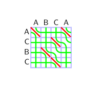
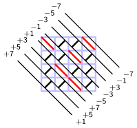
Example 10.4.
Figure 10.1 illustrates Definition 10.3 on an alignment dag for strings , . Subfigure 10.1a shows the alignment dag . Following our usual colour conventions, the diagonal edges of weight are shown in red, and the diagonal edges of weight are omitted. Subfigure 10.1a also shows the reduced seaweed braid laid over the alignment dag . Subfigure 10.1b shows in black the corresponding transposition network, laid diagonally over . By Definition 10.3, a cell contains a comparator, if and only if it does not contain a red diagonal edge. ■
Let us denote the input and output arrays of a transposition network by and , respectively. Assuming all input values of the network are distinct, each value traces a well-defined path through the network. We write , if the input ends up as the output .
Although a transposition network is in general neither merging nor sorting, it is still useful to consider its operation on a certain type of input. Let the input array be anti-sorted (i.e. sorted in decreasing order). It turns out that, given such an input, the operation of the network emulates seaweed combing, and the resulting bijection coincides with the bijection defined by the semi-local seaweed matrix .
Theorem 10.5.
Consider an alignment dag and the corresponding transposition network . For all , , we have , if and only if . □
Proof.
Consider any pair of input values in . Initially, these two values are anti-sorted. Assume that the two values in question meet at some comparator. If by that point their paths have not yet crossed, then they arrive at the comparator anti-sorted, and leave it sorted, so the two paths cross for the first time. Otherwise, the two paths have previously crossed once, therefore the values arrive and leave the comparator sorted, and their paths never cross again.
Since the comparators are located in mismatch cells of , the described operation of each comparator is equivalent to seaweed combing (Algorithm 5.1). Therefore, the paths of the values correspond to the seaweeds in the resulting reduced seaweed braid, and the output of is described in terms of the seaweed matrix as claimed. ■
Example 10.6.
Figure 10.1 illustrates the connection between seaweed braids and transposition networks, as described by Theorem 10.5. Subfigure 10.1a shows the reduced seaweed braid obtained by seaweed combing (Algorithm 5.1), laid over the alignment dag . Subfigure 10.1b shows an anti-sorted input array of distinct values, and the corresponding output array. Each value in Subfigure 10.1b traces a path through the network; the paths are not shown explicitly, but can be reconstructed by running the network “by hand”. Every path turns out to be identical to the layout of the corresponding seaweed in Subfigure 10.1a. ■
Extending Theorem 10.5, it is natural to consider the situation where the input values to a transposition network are anti-sorted, but not necessarily distinct. An extreme case of that is an anti-sorted binary input: a sequence of ones, followed by a sequence of zeros. While in this case, the information on semi-local LCS scores is lost, it turns out that the output still contains sufficient information to obtain the ordinary (global) LCS score.
Theorem 10.7.
Consider an alignment dag and the corresponding semi-local seaweed matrix . Let the transposition network operate on an anti-sorted input array , consisting of -values and -values:
Let be the output array of . Then we have
□
Proof.
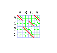
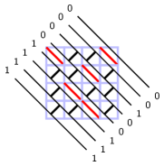
Example 10.8.
Figure 10.2 illustrates Theorem 10.7 on the same pair of strings as Figure 10.1. Subfigure 10.2a shows the seaweed braid of Subfigure 10.1a, laid over the alignment dag . The seaweeds originating at the top (respectively, the left-hand side) of the dag are shown by solid (respectively, dotted) lines. Subfigure 10.2b shows the transposition network of Subfigure 10.1b, laid over the alignment dag . The network is given an anti-sorted binary input. The path of each -value (respectively, -value) corresponds to a solid (respectively, dotted) seaweed. We have
as claimed by Theorem 10.7. ■
10.2 Parameterised LCS
An algorithm’s complexity is most commonly defined to be a function of a single argument: the input size. However, in the pursuit of efficiency, algorithms may also be designed to be sensitive to various other parameters of the input. In the context of string comparison, the two most relevant parameters are:
-
the input strings’ alignment score; we consider primarily the LCS score ;
-
the input strings’ edit distance; we consider primarily the LCS distance .
In this section, we study algorithms for the LCS problem that are sensitive to these parameters. We consider low-similarity and high-similarity LCS algorithms. The running times of such algorithms are parameterised respectively by and , so that advantage can be taken of the low value of a parameter. More generally, one can also use weighted alignment scores or weighted edit distances (e.g. the Levenshtein distance) as parameters.
As we aim for algorithms that, for a low value of the parameter, run substantially faster than , we cannot afford to perform all the pairwise comparisons of characters from each string. As in Section 5.2, we assume a character comparison model that allows comparison outcomes “equal”, “less than” and “greater than”, so that the “missing” comparisons can be obtained by transitivity, and algorithms with running time become possible.
For simplicity, we ignore the trivial cases (the two input strings have no characters in common) and (the two input strings are identical). As usual, we denote the alphabet size by . Without loss of generality, we assume .
Low-similarity comparison (sensitive to low ).
In this type of comparison, the overall number of matching character pairs will be low. To locate these matching pairs effectively, the input strings and are preprocessed into a data structure that allows efficient queries defined by the string identification problem [2, 96, 151]. The preprocessing builds a binary search tree on each input string, and returns a partitioning of both and into character equality classes. This preprocesing procedure runs in time (respectively, ).
After the preprocessing, the low-similarity LCS problem can be solved by one of the algorithms due to Hirschberg [95], Hsu and Du [96] (see also Apostolico [13]), Apostolico and Guerra [17]. All these algorithms run in time . Apostolico, Browne and Guerra [16] proposed another algorithm that requires no preprocessing, and runs in time and linear space.
High-similarity comparison (sensitive to low ).
In this type of comparison, the overall number of matching character pairs may be as high as . However, an efficient high-similarity LCS algorithm may not need to look at all these matches; speaking informally, a good algorithm “will know where to look for relevant matches”. In fact, it is sufficient to consider character matches overall. In contrast to low-similarity comparison, there is no need for preprocessing the input strings.
Flexible comparison (sensitive to both low and low ).
This type of comparison can be achieved by preprocessing the input string as for low-similarity comparison, and then running both comparison types alongside each other. However, dedicated flexible comparison algorithms have also been proposed. In particular, the flexible LCS algorithm by Hirschberg [95] runs in time , and one by Rick [151] in time and linear space.
We now describe an algorithm based on the comparison network method. The algorithm is sensitive to both parameters and , providing flexible LCS computation efficient in both the low- and the high-similarity case. Our algorithm matches existing flexible-LCS algorithms in running time. We call it the waterfall algorithm.
We preprocess input strings to build a data structure for efficient querying of the matches, and also match successor queries: given , , find lowest such that .
Algorithm 10.9.
(Parameterised LCS: The waterfall algorithm)
strings , of length , , respectively.
the LCS score .
The algorithm is based on transposition network with binary input, as described by Theorem 10.7. Such a network can be evaluated efficiently as follows. The dag is processed row-by-row. Instead of performing binary value comparisons within individual mismatch cells of a given row of cells, we partition the row into contiguous horizontal blocks, and combine the comparisons within each block into a single constant-time operation. A block may contain both match and mismatch cells; as we move vertically from one dag row to the next, the blocks may split or merge. We keep track of each block’s endpoints in a parameter-sensitive way, achieving an overall speedup whenever either of the parameters , is low.
Let us now fill in the details. Consider a row of nodes in the alignment dag , corresponding to a fixed index . The nodes in this row are connected by horizontal edges, each of which is crossed by a single wire of the transposition network . Hence, when running the network on a binary input as in Theorem 10.7, each row of nodes corresponds to a sequence of binary values. We regard this sequence as partitioned into contiguous runs of -values, called blocks, alternating with contiguous runs of -values, called gaps. We only need to deal explicitly with the blocks, leaving the processing of gaps implicit (hence the block/gap terminology). If the input strings happen to be highly dissimilar or highly similar, i.e. the respective parameter or is low, then every dag row will have only a small number of blocks (and gaps).
Consider the operation of the transposition network row by row, moving downwards across the alignment dag. In the top row of nodes , we have a single block of -values coming as input to the network, with index set spanning the full row .
Now, given a fixed row of cells , consider a transition from its top boundary to its bottom boundary . Given the endpoints of all blocks in row of nodes , we need to find the endpoints for the blocks in row of nodes . This transformation of endpoints can be achieved in two phases: block splitting and block merging.
Consider a block in row of nodes , spanning the index set . Let be the index of the leftmost match cell (if one exists) immediately below the given block: . If index exists, then block is split at this index into a pair of subblocks:
-
the left subblock , which is empty if , and consists of the whole block if index does not exist; this subblock is kept unchanged in row of nodes ;
-
the right subblock ; this subblock is shifted by one unit to the right, forming a new block in row of nodes (unless , in which case the rightmost -value is considered to be “shifted out” off the right boundary of the dag, and the resulting new block is ).
A unit-length gap is created between the two subblocks in row . The gap at the right of the right subblock (which exists in row , unless ) is reduced by one unit in row .
This occurs whenever a gap between two blocks has been closed (reduced to length ) as a result of shifting a subblock in the previous splitting phase. Suppose that subblock shifting has resulted in a pair of touching blocks and in row . Then, we merge them into a single block . Note that the left touching block must have been split off the right-hand side of a larger block in the preceding splitting phase. Therefore, blocks can only merge in pairs: it is impossible for three or more blocks to merge together in the same merging phase. Upon the completion of all block merging, we have the correct block endpoints in row of nodes .
After all the rows of cells in the alignment dag have been processed, the values , are obtained as follows:
-
for , the values correspond to the sequence of blocks and gaps resulting from the final iteration of the split/merge procedure;
-
for , the values correspond, in reverse order, to the sequence of -values (and, implicitly, -values) “shifted out” off the right boundary of the dag in each of the iterations of the split/merge procedure.
The LCS score of the input strings , can now be obtained by Theorem 10.7.
We now need to show that the described algorithm emulates correctly the operation of the transposition network on binary input, as defined by Theorem 10.7. Consider the operation of the algorithm in row of cells . The operation within an individual cell depends on whether the top edge of the cell belongs to a left subblock (which can be the whole block in case it does not get split), a right subblock, or a gap. We also need to consider separately the leftmost cell under a right subblock (the “subblock splitting cell”), and the leftmost cell under a gap following a right subblock (the “gap filling cell”). We thus have the following cases for a cell’s operation (where L = “left”, R = “right”, T = “top”, B = “bottom”).
| Cell’s top edge | Input | Output | Match? | ||
| L | T | B | R | ||
| In L subblock | 1 | 0 | 0 | 1 | mismatch |
| Leftmost in R subblock | 1 | 0 | 1 | 0 | match |
| Other in R subblock | 0 | 0 | 0 | 0 | either |
| Leftmost in gap after R subblock | 0 | 1 | 0 | 1 | either |
| Other in gap | 1 | 1 | 1 | 1 | either |
It is now straightforward to check that the input-output relationship defined by the above table is consistent with the operation of all the individual comparators in the network , and that the algorithm’s overall running time is . ■
The name “waterfall algorithm” for Algorithm 10.9 is justified by the following interpretation. Let us think of the -values as a non-compressible water that flows through the alignment dag under gravity. The blocks of adjacent -values correspond to water jets that may split or merge while flowing through the dag. Initially, there is just a single jet of width , falling vertically down through the top boundary of the dag. The diagonal match edges are rocks that form barriers for the water: whenever a jet hits a rock in its path, it gets displaced by one unit to the right, following the rock’s inclination. This displacement may result in a jet splitting at the top-left tip of the rock; the displaced water may also fill the gap to its right and merge with a jet falling vertically just beyond that gap. The amount of water that emerges from the dag at its right-hand side (respectively, at its bottom) equals the LCS score (respectively, the LCS distance ) of the input strings.
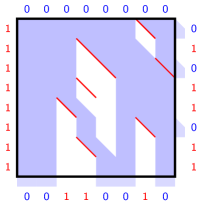
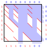
Example 10.10.
Figure 10.3 illustrates two separate runs of the waterfall algorithm (Algorithm 10.9):
-
Subfigure 10.3a shows the low-similarity case, with input strings , ;
-
Subfigure 10.3b shows the high-similarity case, with input strings , .
Following our usual convention, the diagonal edges in match cells are shown in red. The rest of the alignment dag, as well as the input strings, are kept implicit. The anti-sorted input to the transposition network is represented by the sequences of red -values and blue -values along the left (respectively, the top) boundary of the alignment dag.
The iterative procedure of block splitting and merging is shown by filling in the interior of the alignment dag with blue and white pattern as follows. Every horizontal edge in the alignment dag corresponds to a blue (respectively, white) streak in the pattern, whenever that edge is crossed by an (implicit) wire carrying a - (respectively, -) value. Therefore, for each row index in the dag, the corresponding sequence of blocks and gaps is represented by a sequence of continuous blue and white streaks in a horizontal line at level . The transition of block sequences between every pair of successive rows is shown by connecting the corresponding pairs of blue streaks with a blue strip. For the vertical (respectively, diagonal) transition of a single -value, the connecting strip has the shape of a unit square (respectively, unit-width parallelogram).
The output of the transposition network is represented by the mixed sequence of red -values and blue -values along the bottom and right boundaries of the alignment dag. Each output -value is also shown by a blue tab. By Theorem 10.7, we have
Just as the splitting/merging procedure in Algorithm 10.9 is not symmetric with respect to blocks and gaps, so the pattern in Figure 10.3 is not symmetric either with respect to horizontal and vertical directions, or with respect to - and -values. For this reason, while the blocks are represented by the usual blue colour, the gaps are left uncoloured (i.e. are represented by the “background” white). The red colour, which we would normally use to represent -values, is not present in the pattern. ■
Parameterised LCS algorithms are closely related to threshold LCS algorithms. Here, a threshold value for the parameter or is given, and the algorithm is required to output the LCS score of the input strings, as long as this value is below the threshold, or to report “excess”, if the LCS score (respectively, LCS distance) exceeds the threshold; in the latter case, there is no requirement for the score to be output explicitly. In general, a threshold algorithm can be obtained from a parameterised algorithm by setting an appropriate time-out threshold as a function of the parameter threshold, and reporting “excess”, if the algorithm’s running time exceeds the time-out threshold. Alternatively, a threshold LCS algorithm can be obtained from the waterfall algorithm (Algorithm 10.9) by reporting “excess”, if the current number of blocks exceeds the threshold value for (respectively, ).
10.3 Bit-parallel LCS
The most efficient practical method for computing the (global) LCS score for a pair of strings is by bit-parallel algorithms. These algorithms take advantage of bitwise Boolean operations on bit vectors available in modern processors, often in combination with arithmetic operations on the same vectors as integers. We denote by the word (standard bit vector) length; in modern general-purpose processors, word length is often .
Early bit-parallel string comparison algorithms were given by Allison and Dix [10] and by Myers [139]. Crochemore at al. [56] proposed an efficient bit-parallel LCS algorithm, running in time . For every cells of the alignment dag , the algorithm only performs five elementary operations (one arithmetic and four Boolean). Hyyrö [100] improved this to four operations (two arithmetic and two Boolean).

0 1 0 1 0 1 0 1 0 0 1 1 0 0 1 1 0 0 0 0 1 1 1 1 0 1 1 1 0 0 1 1 0 0 0 1 0 1 0 1

| 0 | 1 | 0 | 1 | 0 | 1 | 0 | 1 | |
| 0 | 0 | 1 | 1 | 0 | 0 | 1 | 1 | |
| 0 | 0 | 0 | 0 | 1 | 1 | 1 | 1 | |
| 0 | 1 | 1 | 0 | 0 | 0 | 1 | 1 | |
| 0 | 0 | 0 | 1 | 0 | 1 | 0 | 1 |
Both algorithms [56, 100] can be viewed as an implementation of a binary transposition network, described in Section 10.1, by standard bit-parallel processor instructions. Figure 10.4 shows the main idea of such an implementation for the algorithm of [56]. Consider a cell in a binary transposition network, and let us denote its input bits by , , and its output bits by , , as shown in Subfigure 10.4a. Let us denote by an extra input bit, which takes value if and only if the current dag cell is a match cell. The operation of a network cell is fully described by the truth table in Subfigure 10.4b.
Now consider a Boolean circuit shown in Subfigure 10.4c. The circuit consists of an -gate and a full adder element, which adds its three input bits arithmetically, and returns the sum as two separate output bits. Let us again denote the input bits by , , , and the output bits by , . Then, the circuit computes a Boolean-arithmetic expression
The operation of such a circuit is fully described by the truth table in Subfigure 10.4d.
Note that the truth tables in Subfigures 10.4b and 10.4d differ in just the one highlighted bit. This difference can be corrected by two extra Boolean operations, resulting in a Boolean-arithmetic expression that fully implements the operation of a single transposition network cell:
| (10.1) |
Now consider a row of cells in the alignment dag , assuming for the moment . Let denote a word variable that will hold the input , and then the output , for each cell, least significant bit first. Likewise, let denote a word constant that holds the match parameter for each cell, least significant bit first. (The input and output will not be represented explicitly, but will instead correspond to a propagating carry bit in word integer addition, from the least significant bit all the way to the most significant bit.) The operation of the transposition network in the given row of cells corresponds to evaluating an expression
| (10.2) |
which is obtained from (10.1) by identifying the output of each cell with the input of the next cell in the row. Here, the Boolean operations are bitwise, and the addition is on integers represented by the words. Note that for an exact correspondence with (10.2), the roles of 0-values and 1-values in the waterfall algorithm (Algorithm 10.9) must be exchanged (or, alternatively, the cells must be composed into words by columns, rather than by rows).
If , then each row of the alignment dag is partitioned into words of length . In this case, expression (10.2) needs to be modified to allow carry propagation from each word to the next word in its row.
The described bit-parallel approach can be extended to provide even more efficient string comparison in the case of highly similar strings. We consider the threshold version of the high-similarity LCS problem, as described in Section 10.2. Let denote a threshold on , i.e. the LCS distance between the input strings , . We assume for simplicity that the value is odd, and that . Under these assumptions, a highest-scoring path in the alignment dag must lie strictly within a symmetric diagonal band of width , unless exceeds . Hence, the waterfall algorithm (Algorithm 10.9) can be modified as follows. First, we ignore all character matches outside the band, as well as on the band’s lower-left and upper-right boundaries. We also ignore all the (explicit) input 0-values and all the (implicit) input 1-values outside the band; therefore, we only have (explicit) input 0-values at the top of the band, and (implicit) input 1-values at the left-hand side of the band. Finally, we create artificial separator matches along the bottom-left boundary of the band. The LCS score can be obtained by counting the output 0-values at the bottom of the band (or, symmetrically, the output 1-values at the right-hand side of the band). The algorithm reports “exceed”, if all the input 0-values are output at the bottom of the band. The algorithm runs in time .
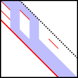
Figure 10.5 shows a run of the resulting high-similarity bit-parallel waterfall algorithm, for . The visual conventions are similar to those in Figures 10.3a, 10.3b. Note that the band is of width , and that there are input 0-values at the band’s top. Both these values end up as output 0-values at the band’s bottom, hence the algorithm returns “exceed” in the given run.
The described algorithm is particularly easy to implement when the bandwidth . In such a case, every row of the band fits into a single word. The bit-parallel five- (respectively, four-) instruction sequence of either of [56, 100] can be used; the only modification required is an extra shift instruction in each row, to account for the band right-shifting by when moving to the next row.
Still further optimisation is possible in the case of multi-string comparison. This type of comparison has been considered e.g. by by Hyyrö et al. [101]. Here, we asked to compute the LCS score for string against each of the strings , …, , all of length . We assume that we are given a single threshold on all , . As before, we assume for simplicity that the value is odd, and that . The problem can be solved by independent runs of the high-similarity bit-parallel waterfall algorithm. However, it is possible to combine these runs into a single bit-parallel computation, where in each step, we evaluate a single row from every one of the bands. The bands are packed together in a single super-band of width ; individual bands within the super-band are separated by diagonals of separator matches.
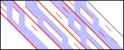
Figure 10.6 shows a run of the resulting high-similarity bit-parallel multi-string waterfall algorithm, for and . The leftmost band (band ) is identical to the band in Figure 10.5. The algorithm returns “exceed” for bands , , . For band , we have a single 0-value output at the bottom of the band, hence by Theorem 10.7.
Finally, note that all the described techniques for bit-parallel string comparison are compatible with integer-weighted alignment, by application of the blow-up technique described in Section 6.1. For example, we can obtain bit-parallel algorithms for Levenshtein alignment score (or, symmetrically, Levenshtein edit distance) by blowing up the alignment dag by a factor of in each dimension.
Chapter 11 Beyond semi-locality
In this chapter, our aim is to extend the approach of the previous chapters beyond semi-local string comparison, with the ultimate goal of efficient fully-local string comparison. We study several problems, where for each of the two input strings, their various substrings are selected for pairwise comparison. This type of string comparison is arguably the most important, in particular for biological applications. However, it is also the most computationally expensive, therefore there is particular need for efficient algorithms.
This chapter is organised as follows. In Section 11.1, we introduce the window-substring and window-window LCS problems, and give an efficient algorithm for these problems. This algorithm provides a refinement for the standard dot plot method, by allowing window-window string comparison based on the LCS score, rather than the less sensitive Hamming score. In Section 11.2, we introduce the quasi-local LCS problem, which generalises the semi-local, window-substring and window-window LCS problems, and give an efficient algorithm for this problem. By application of this algorithm, in Section 11.3 we obtain an algorithm for sparse spliced alignment under an arbitrary rational edit distance metric, which improves on existing algorithms for this problem.
11.1 Window-local LCS and alignment plots
Numerous methods of local string comparison have been proposed in the past. The Smith–Waterman–Gotoh algorithm [160, 89] allows one to obtain the highest-scoring pair across all substring pairs in the two input strings. It can also be generalised to report all substring pairs scoring above a certain threshold. A significant drawback of the Smith–Waterman–Gotoh algorithm is that it generally favours long, less precise substring alignments over short, more precise ones (as noted e.g. by Arslan et al. [20]). The quality of the alignment is also dependent on the scoring scheme: for example, for the simplest LCS score, the algorithm only provides the trivial global comparison, so the method is generally only useful for weighted alignment scores with sufficiently high penalties (negative score weights) for gaps.
The drawbacks of the Smith–Waterman–Gotoh approach have been addressed by the techniques of normalised alignment by Arslan et al. [20], and length-constrained alignment by Arslan and Eğecioğlu [19]. Such methods typically have very high computational cost. To reduce this cost, various approximation algorithms for the same problems have been suggested (see [19]).
An alternative approach, is to obtain local comparison of two strings by computing an alignment plot, i.e. an exhaustive set of alignments for pairs of fixed-length windows in both sequences. A similar method is used by Rasmussen et al. [147], where an algorithm for local alignment in fixed-length windows in described. The difference of our approach from that of [147] is that the latter is designed to be very efficient when the similarity threshold is high, but becomes prohibitively expensive when looking for relatively low-similarity matches (e.g. 70% similarity). In contrast, our method works equally efficiently for any similarity threshold.
Recall from Section 5.5 that, given a fixed parameter , we call a substring of length a -window in the corresponding string. String comparison in windows has a long history. One of its early instances is dot plots (also known as diagonal plots or dot matrices), introduced by Gibbs and McIntyre [85] and by Maizel and Lenk [130] (see also Crochemore et al. [55]). In addition to numerical scores, dot plots provide a convenient visualisation of string comparison. In the context of dot plots, processing a pair of windows is usually referred to as filtering. The standard filtering method compares every -window of string against every -window of string in terms of their Hamming score, i.e. the count of matching character pairs under a rigid alignment model, where every character must be aligned (resulting in either a match or a mismatch), and no gaps are allowed. A Hamming-filtered dot plot can be computed in time by the algorithm of [130, 135]. This algorithm has been implemented in several software packages (see e.g. [161, 148, 50]). A faster suffix-tree based algorithm has been proposed and implemented by Krumsiek et al. [118]. Enhancement of the dot plot approach have been proposed by Huang and Zhang [98] and by Putonti et al. [146].
In contrast with the Smith–Waterman–Gotoh algorithm, the dot plot method gives the user more flexibility to select the biologically significant substring alignments, by providing all the local scores between fixed-size windows of the input strings. However, the Hamming scoring scheme used by this method within each window pair is less sensitive than even the LCS score, and especially than the weighted alignment score used by Smith–Waterman–Gotoh. This tradeoff motivates us to combine the best features of the two approaches in the following definition.
Definition 11.1.
Given strings , , and a window length , the window-window (respectively, window-substring) LCS problem asks for the LCS score of for every -window in against every -window (respectively, every substring) in . □
The window-window LCS problem can be seen as a refinement of the dot plot method and a complement to the Smith–Waterman–Gotoh method. As in the dot plot method, we compute all window-window comparison scores between the input strings. However, instead of the Hamming score, our method is based on the LCS score, and is therefore potentially more sensitive. The method can be further extended to use weighted alignment scores. By analogy with Hamming-filtered dot plots, we call the resulting matrix of window-window alignment scores an alignment-filtered dot plot, or simply an alignment plot. Recently, the alignment plot method has been applied to the detection of alignment-conserved regions in DNA by Picot et al. [144]. Computation of an alignment plot is also a key subroutine in the approximate repeat searching method by Federico et al. [75].
A solution to the window-substring LCS problem can be represented in space by the data structure of Theorem 2.15, built on the string-substring seaweed matrix for each window of against . An individual window-substring LCS score query can be performed on this data structure by Theorem 2.15 in time . The same data structure can be used to obtain explicitly a solution to the window-window LCS problem in time , by performing a diagonal batch query directly on each of the string-substring seaweed matrices. Thus, string-substring seaweed matrices provide a unified solution for both the window-substring and the window-window LCS problems.
A straightforward algorithm for the window-substring (and therefore also window-window) LCS problem can be obtained by solving the semi-local LCS problem independently to each window of string against whole string . Using Algorithm 5.1 (seaweed combing) as a subroutine, the resulting algorithm runs in time . If window length is sufficiently large, the running time can be improved slightly by the micro-block speedup (Algorithm 5.3).
We now give an algorithm for the window-substring (and window-window) LCS problem that improves substantially on the above approach, and matches the asymptotic running time of both the Hamming-scored dot plot and the Smith–Waterman–Gotoh methods.
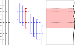
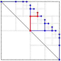
Algorithm 11.2 (Window-substring LCS).
strings , of length , , respectively; window length .
nonzeros of the string-substring seaweed matrix for every -window , , against full string .
We call a substring canonical, if , where is an arbitrary power of , , and , are both multiples of . In particular, every individual character of is a canonical substring with . Every substring of of length can be decomposed into a concatenation of at most canonical substrings.
In the following, by processing a substring , we mean computing the string-substring seaweed matrix .
We process all canonical substrings of by the following recursive procedure.
For every canonical substring of length , matrix is computed by Algorithm 5.1 (seaweed combing) on strings and , of length and respectively.
For every canonical substring of length , we have , where , are both canonical substrings of length . By Theorem 4.19, we have
The implicit matrix distance product can be computed by Theorem 4.21.
Let be an arbitrary power of , . We define -window to be a substring , such that , and and are both multiples of . Intuitively, is the amount of shift between two successive -windows, and is the number of different -windows that cover any single character in the string (except possibly near its boundaries). Note that a -window is the same as a -window, and an -window is the same as a canonical substring of length . Given parameters , , we solve the problem of processing all -windows by the following recursive procedure.
For any , all -windows are canonical substrings of length , therefore they have already been processed in the first phase.
-
Case of even. First, we call the second phase recursively to process all -windows. Now consider an -window . We have the decomposition
(11.1) Observe that the prefix and the suffix are both -windows; also, the suffix and the prefix are both -windows. Therefore, we can now process all -windows as follows:
(11.2) where the choice between the two alternatives can be made arbitrarily.
-
Case of odd. We first call the second phase recursively to process all -windows (in other words, “every other -window”). Now consider an -window . As before, we have the decomposition (11.1), where the prefix and the suffix are both -windows. Furthermore, if is even and and is odd, then the prefix is a -window. Likewise, if is odd and and is even, then the suffix is a -window. The suffix and the prefix are both -windows. Therefore, we can now process all -windows as follows:
(11.3) Note that the equations in (11.3) are identical to the ones in (11.2), but the choice between the alternatives is now determined by the parity of the values , . The two alternatives in (11.3) are exhaustive: must be odd, since is odd and is a power of .
The implicit matrix distance products in (11.2), (11.3) are computed by Theorem 4.21. In each case, the product is between two string-substring seaweed matrices: one for substring or , already processed by the recursive call, and the other for a canonical substring or .
Starting at the top recursion level, the number of seaweed matrix multiplications doubles in every subsequent level down the recursion. The running time for each matrix multiplication is , where the parameter halves in every subsequent level of recursion. Therefore, the running time of the whole phase is dominated by the bottom level of the recursion, where we have matrix multiplications, each running in time . The running time of the whole phase is .
Starting at the top recursion level, the number of seaweed matrix multiplications halves in every recursion level where the parameter is odd, which is at least a half of all the recursion levels. In a recursion level where is even, the number of matrix multiplications does not change. The running time for each matrix multiplication is , where the parameter doubles in every recursion level where the parameter is odd, and does not change in every recursion level where the parameter is even. Therefore, the running time of the whole phase is dominated by the top level of the recursion, where we have matrix multiplications, each running in time . The running time of the whole phase is .
The running time for both the first and the second phase, and therefore the overall running time, is . ■
Note that the asymptotic running time of Algorithm 11.2 is independent of the window length .
Example 11.3.
Figure 11.1 shows an execution of Algorithm 11.2 on string of length with window size , against string of arbitrary length. Subfigure 11.1a shows the canonical substrings of of lengths , , , , in black, and windows of length in blue. For each window, the figure shows its decomposition into canonical substrings. For one of the windows, highlighed in thick red, the corresponding area is outlined in the alignment dag. Subfigure 11.1b represents substrings of by points in the plane, and the decompositions into canonical substrings by a forest of trees. Each window corresponds to a leaf of a decomposition tree. The canonical substrings in a decomposition of the window correspond to the edges on the path from this leaf to the root of the tree; for the window shown in red, its corresponding path is also highlighted in red. The leaves, internal nodes and roots of decomposition trees are shown respectively by diamonds, circles and squares. ■
11.2 Quasi-local LCS
We now generalise window-local string comparison as follows. Suppose that we are given an arbitrary set of prescribed substrings of various lengths in string . We assume that all the prescribed substrings are non-empty, and denote their number by , .
Definition 11.4.
Given strings , , the quasi-local LCS problem asks for the LCS score of every prescribed substring in against every substring in . □
The quasi-local LCS problem includes as special cases the semi-local, window-window, window-substring and fully-local LCS problems, as well as length-constrained local alignment considered by Arslan and Eğecioğlu [19]. The solution of the quasi-local LCS problem can be represented in space by the data structure of Theorem 2.15, built on the string-substring seaweed matrix for each prescribed substring of against . An individual quasi-local LCS score query can be performed on this data structure in time .
A straightforward algorithm for the quasi-local LCS problem can be obtained by applying Algorithm 5.1 (seaweed combing) independently to each prescribed substring against whole string . The resulting algorithm runs in time . If all the prescribed substrings are sufficiently long, then the running time can be improved slightly by the micro-block speedup (Algorithm 5.3).
We now give an algorithm for the quasi-local LCS problem that improves substantially on the above approach.
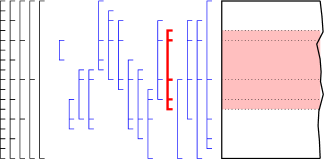
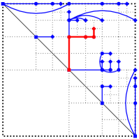
Algorithm 11.5 (Quasi-local LCS).
strings , of length , , respectively; a set of endpoint index pairs for the prescribed substrings in .
nonzeros of the string-substring seaweed matrix for every prescribed substring of string against full string .
The algorithm structure is similar to the one of Algorithm 11.2.
As in Algorithm 11.2.
First, we remove from consideration all canonical prescribed substrings, since they have already been processed in the first phase. We then process all the remaining prescribed substrings of by the following recursive procedure. Let be a parameter, assumed to be a power of . Initially, we set . At every level of recursion, the endpoint indices of the prescribed substrings are multiples of .
In this case, the problem is trivial.
We call the second phase procedure recursively with the parameter , and the following set of prescribed substrings. For each currently prescribed non-canonical substring , the corresponding new prescribed substring in the recursive call is , unless this substring is empty. Informally, we round and to a multiple of ; index is rounded up and index down. Note that different currently prescribed substrings may correspond to the same new prescribed substring in the recursive call.
The recursive call results in the processing of all the prescribed substrings where , are multiples of ; in other words, where and are both even. We then process all remaining prescribed substrings as follows:
The seaweed matrix products are computed by Theorem 4.21. In each case, the product is between two or three string-substring seaweed matrices: one matrix for substring , or , already processed by the recursive call; and the other one or two matrices for canonical substrings and/or .
As in Algorithm 11.2, the total running time of this phase is .
In every level of the recursion, the number of matrix multiplications is at most . The running time for each matrix multiplication is at most . The recursion has levels. Therefore, the running time is dominated by the top level of the recursion, where we have matrix multiplications, each running in time . Therefore, the running time of the whole phase is .
For values of close to the fully-local case , a sharper analysis is possible. In this case, the running time of the whole phase is .
The overall running time is dominated by the second phase, and is therefore . For values of close to , the running time is . ■
Note that in the fully-local case, i.e. the case where all nonempty substrings of are prescribed, the same asymptotic time can be obtained by solving the prefix-substring LCS problem independently for each of the nonempty suffixes of string . Each of these prefix-substring LCS instances can be solved by a separate run of Algorithm 5.1 (seaweed combing).
11.3 Sparse spliced alignment
Assembling a gene from candidate exons is an important problem in computational biology. Several alternative approaches to this problem have been developed over time. One of such approaches is spliced alignment by Gelfand et al. [83] (see also [90]), which scores different candidate exon chains within a DNA sequence by comparing them to a known related gene sequence. In this method, the two sequences are modelled respectively by strings , of lengths , respectively. A subset of substrings in string are marked as candidate exons. The comparison between sequences is made by string alignment. The algorithm for spliced alignment given in [83] runs in time .
In general, the number of candidate exons may be as high as . The method of sparse spliced alignment makes a realistic assumption that, prior to the assembly, the set of candidate exons undergoes some filtering, after which only a small fraction of candidate exons remains. Kent et al. [111] give an algorithm for sparse spliced alignment that, in the special case , runs in time . By a direct application of the quasi-local LCS problem (Section 11.2), the running time can be reduced to . Sakai [156] gave an improved algorithm, running in time .
For higher values of , all the described algorithms provide a smooth transition in running time to the dense case . In this case, the algorithms’ running time is asymptotically equal to the algorithm of [83].
We now describe an algorithm for sparse spliced alignment, based on the approach of [156]. We keep the notation and terminology of the previous sections; in particular, candidate exons are represented by prescribed substrings of string . We say that substring precedes substring , if . A precedence chain of substrings is a chain in the partial order of substring precedence. We identify every precedence chain with the string obtained by concatenating all its component substrings in the order of precedence.
The algorithm uses a generalisation of the standard network alignment method, equivalent to the one used by [111]. For simplicity, we describe the algorithm under LCS score; using the blow-up technique of Section 6.1, the algorithm can be generalised to an arbitrary alignment score with rational weights.
Algorithm 11.7 (Sparse spliced alignment).
strings , of length , , respectively; a set of endpoint index pairs for the prescribed substrings in .
the precedence chain of prescribed substrings in , giving the highest LCS score against string .
The algorithm runs in two phases.
As in Algorithm 11.2.
The problem is now solved by dynamic programming as follows. Let denote the highest LCS score across all precedence chains of prescribed substrings in prefix string , taken against prefix string . With each , we associate the integer vector . We initialise as the zero vector. We then compute the vectors , , in the order of increasing . Let , , …, be all the prescribed substrings of terminating at index . We have
| (11.4) |
for all .
The matrices , , …, do not need to be computed explicitly. Instead, it is straightforward to compute each of the vector-matrix distance products in (11.4) by up to instances of implicit vector-matrix distance product, using the decomposition of each of , , …, into up to canonical substrings, along with the corresponding seaweed matrices obtained in the first phase.
The solution score is now given by the value . The solution precedence chain of prescribed substrings can be obtained by tracing the dynamic programming sequence backwards from vector to vector .
As in Algorithm 11.2, the total running time of this phase is .
For each of prescribed substrings of , we execute up to instances of implicit matrix-vector distance multiplication. Every such instance runs in time by Theorem 3.15. Therefore, the total running time of this phase is .
The overall running time of the algorithm is dominated by the second phase, and is therefore . ■
Chapter 12 Conclusions
We have presented a number of existing and new algorithmic techniques and applications related to semi-local string comparison. Our approach unifies a substantial number of previously unrelated problems and techniques, and in many cases allows us to match or improve existing algorithms.
A number of questions related to the semi-local string comparison framework remain open. In particular, it is not yet clear whether the framework can be extended to arbitrary real costs, or to sequence alignment with non-linear gap penalties.
In summary, semi-local string comparison turns out to be a powerful algorithmic technique, which unifies, and often improves on, a number of previous approaches to various substring- and subsequence-related problems. It is likely that further development of this approach will give it even more scope and power.
Chapter 13 Acknowledgement
This work was conceived in a discussion with Gad Landau in Haifa. The imaginative term “seaweeds” was coined by Yuri Matiyasevich during a presentation by the author in St. Petersburg. I thank Elżbieta Babij, Philip Bille, Paweł Gawrychowski, Tim Griffin, Dima Grigoriev, Peter Krusche, Gad Landau, Victor Levandovsky, Sergei Nechaev, Dima Pasechnik, Luís Russo, Andrei Sobolevski, Nikolai Vavilov, Oren Weimann, and Michal Ziv-Ukelson for fruitful discussions, and many anonymous referees for their comments that helped to improve this work.
Bibliography
- [1] A. Aggarwal, M. M. Klawe, S. Moran, P. Shor, and R. Wilber. Geometric applications of a matrix-searching algorithm. Algorithmica, 2(1):195–208, 1987.
- [2] A. V. Aho, D. S. Hirschberg, and J. D. Ullman. Bounds on the complexity of the longest common subsequence problem. Journal of the ACM, 23:1–12, 1976.
- [3] A. V. Aho, J. E. Hopcroft, and J. D. Ullman. The Design and Analysis of Computer Algorithms. Addison-Wesley, 1976.
- [4] M. Ajtai, J. Komlós, and E. Szemerédi. An sorting network. In Proceedings of the 15th ACM STOC, pages 1–9, 1983.
- [5] M. Ajtai, J. Komlós, and E. Szemerédi. Sorting in parallel steps. Combinatorica, 3(1):1–19, 1983.
- [6] S. W. Al-Haj Baddar and K. E. Batcher. Designing Sorting Networks: A New Paradigm. Springer, 2011.
- [7] M. H. Albert, R. E. L. Aldred, M. D. Atkinson, H. P. van Ditmarsch, B. D. Handley, C. C. Handley, and J. Opatrny. Longest subsequences in permutations. Australasian Journal of Combinatorics, 28:225–238, 2003.
- [8] M. H. Albert, M. D. Atkinson, D. Nussbaum, J.-R. Sack, and N. Santoro. On the longest increasing subsequence of a circular list. Information Processing Letters, 101:55–59, 2007.
- [9] M. H. Albert, A. Golynski, A. M. Hamel, A. López-Ortiz, S. S. Rao, and M. A. Safari. Longest increasing subsequences in sliding windows. Theoretical Computer Science, 321:405–414, 2004.
- [10] L. Allison and T. I. Dix. A bit-string longest-common-subsequence algorithm. Information Processing Letters, 23(5):305–310, 1986.
- [11] C. E. R. Alves, E. N. Cáceres, and S. W. Song. An all-substrings common subsequence algorithm. Discrete Applied Mathematics, 156(7):1025–1035, 2008.
- [12] A. Amir, G. Benson, and M. Farach. Let sleeping files lie: Pattern matching in Z-compressed files. Journal of Computer and System Sciences, 52(2):299–307, 1996.
- [13] A. Apostolico. Remark on the Hsu–Du new algorithm for the longest common subsequence problem. Information Processing Letters, 25(4):235–236, 1987.
- [14] A. Apostolico, M. J. Atallah, and S. E. Hambrusch. New clique and independent set algorithms for circle graphs. Discrete Applied Mathematics, 36:1–24, 1992.
- [15] A. Apostolico, M. J. Atallah, L. L. Larmore, and S. MacFaddin. Efficient parallel algorithms for string editing and related problems. SIAM Journal on Computing, 19(5):968–988, 1990.
- [16] A. Apostolico, S. Browne, and C. Guerra. Fast linear-space computations of longest common subsequences. Theoretical Computer Science, 92(1):3–17, 1992.
- [17] A. Apostolico and C. Guerra. The longest common subsequence problem revisited. Algorithmica, 2(1):315–336, 1987.
- [18] V. L. Arlazarov, E. A. Dinic, M. A. Kronrod, and I. A. Faradzev. On economical construction of the transitive closure of an oriented graph. Soviet Mathematical Doklady, 11:1209–1210, 1970.
- [19] A. N. Arslan and Ö. Eğecioğlu. Approximation algorithms for local alignment with length constraints. International Journal of Foundations of Computer Science, 13(5):751–767, 2002.
- [20] A. N. Arslan, Ö. Eğecioğlu, and P. A. Pevzner. A new approach to sequence comparison: Normalized sequence alignment. Bioinformatics, 17(4):327–337, 2001.
- [21] M. J. Atallah, S. R. Kosaraju, L. L. Larmore, G. L. Miller, and S.-H. Teng. Constructing trees in parallel. In Proceedings of the 1st ACM SPAA, pages 421–431, 1989.
- [22] K. E. Batcher. Sorting networks and their applications. In AFIPS Conference Proceedings, volume 32, pages 307–314. Thompson Book Company, 1968.
- [23] W. W. Bein and P. K. Pathak. A characterization of the Monge property and its connection to statistics. Demonstratio Mathematica, 29:451–457, 1996.
- [24] G. Benson. Tandem cyclic alignment. Discrete Applied Mathematics, 146(2):124–133, 2005.
- [25] J. L. Bentley. Multidimensional divide-and-conquer. Communications of the ACM, 23(4):214–229, 1980.
- [26] L. Bergroth, H. Hakonen, and T. Raita. A survey of longest common subsequence algorithms. In Proceedings of the 7th SPIRE, pages 39–48, 2000.
- [27] S. Bespamyatnikh and M. Segal. Enumerating longest increasing subsequences and patience sorting. Information Processing Letters, 76:7–11, 2000.
- [28] P. Bille, R. Fagerberg, and I. L. Gørtz. Improved approximate string matching and regular expression matching on Ziv-Lempel compressed texts. ACM Transactions on Algorithms, 6(1):3:1–3:14, 2009.
- [29] P. Bille and M. Farach-Colton. Fast and compact regular expression matching. Theoretical Computer Science, 409(3):486–496, 2008.
- [30] P. Bille and I. L. Gørtz. Matching subsequences in trees. Journal of Discrete Algorithms, 7(3):306–314, 2009.
- [31] P. Bille, G. M. Landau, R. Raman, K. Sadakane, Srinivasa Rao Satti, and O. Weimann. Random access to grammar-compressed strings. In Proceedings of the 22nd ACM-SIAM SODA, pages 373–389, 2011.
- [32] A. Björner and F. Brenti. Combinatorics of Coxeter Groups. Number 231 in Graduate Texts in Mathematics. Springer, 2005.
- [33] Miklós Bóna. Combinatorics of Permutations. Discrete Mathematics and Its Applications. Chapman & Hall/CRC, 2004.
- [34] N. Bourbaki. Groupes et algèbres de Lie. Chapitres 4,5 et 6. Hermann, 1968.
- [35] A. S. Buch, A. Kresch, M. Shimozono, H. Tamvakis, and A. Yong. Stable Grothendieck polynomials and K-theoretic factor sequences. Mathematische Annalen, 340(2):359–382, 2008.
- [36] H. Bunke and U. Bühler. Applications of approximate string matching to 2D shape recognition. Pattern Recognition, 26(12):1797–1812, 1993.
- [37] V. Y. Burdyuk and V. N. Trofimov. Generalization of the results of Gilmore and Gomory on the solution of the traveling salesman problem. Engineering Cybernetics, 14:12–18, 1976.
- [38] R. E. Burkard. Monge properties, discrete convexity and applications. European Journal of Operational Research, 176(1):1–14, 2007.
- [39] R. E. Burkard, B. Klinz, and R. Rudolf. Perspectives of Monge properties in optimization. Discrete Applied Mathematics, 70(2):95–161, 1996.
- [40] P. Butković. Max-linear Systems: Theory and Algorithms. Springer Monographs in Mathematics. Springer, 2010.
- [41] S. Cabello and E. W. Chambers. Multiple-source shortest paths in a genus graph. In Proceedings of the 18th ACM-SIAM SODA, pages 89–97, 2007.
- [42] P. Cégielski, I. Guessarian, Y. Lifshits, and Y. Matiyasevich. Window subsequence problems for compressed texts. In Proceedings of CSR, volume 3967 of Lecture Notes in Computer Science, pages 127–136, 2006.
- [43] P. Cégielski, I. Guessarian, and Y. Matiyasevich. Multiple serial episodes matching. Information Processing Letters, 98(6):211–218, 2006.
- [44] T. Chan and M. Pǎtraşcu. Counting inversions, offline orthogonal range counting, and related problems. In Proceeding of ACM–SIAM SODA, pages 161–173, 2010.
- [45] T. M. Chan. More algorithms for all-pairs shortest paths in weighted graphs. In Proceedings of the 39th ACM STOC, pages 590–598, 2007.
- [46] Maw-Shang Chang and Fu-Hsing Wang. Efficient algorithms for the maximum weight clique and maximum weight independent set problems on permutation graphs. Information Processing Letters, 43(6):293–295, 1992.
- [47] Kun-Mao Chao and Louxin Zhang. Sequence Comparison: Theory and Methods, volume 7 of Computational Biology Series. Springer, 2009.
- [48] B. Chazelle. A functional approach to data structures and its use in multidimensional searching. SIAM Journal on Computing, 17:427–462, 1988.
- [49] E. Chen, L. Yang, and H. Yuan. Longest increasing subsequences in windows based on canonical antichain partition. Theoretical Computer Science, 378(3):223–236, 2007.
- [50] CLC bio. CLC Protein Workbench: User Manual, 2006.
- [51] R. Cole and R. Hariharan. Approximate string matching: A simpler faster algorithm. SIAM Journal on Computing, 31(6):1761–1782, 2002.
- [52] J.-P. Comet. Application of max-plus algebra to biological sequence comparisons. Theoretical Computer Science, 293(1):189–217, 2003.
- [53] T. H. Cormen, C. E. Leiserson, R. L. Rivest, and C. Stein. Introduction to Algorithms. The MIT Electrical Engineering and Computer Science Series. The MIT Press and McGraw–Hill, second edition, 2001.
- [54] G. Cormode and S. Muthukrishnan. The string edit distance matching problem with moves. ACM Transactions on Algorithms, 3(1), 2007.
- [55] M. Crochemore, C. Hancart, and T. Lecroq. Algorithms on Strings. Cambridge University Press, 2007.
- [56] M. Crochemore, C. S. Iliopoulos, Y. J. Pinzon, and J. F. Reid. A fast and practical bit-vector algorithm for the Longest Common Subsequence problem. Information Processing Letters, 80(6):279–285, 2001.
- [57] M. Crochemore, G. M. Landau, B. Schieber, and M. Ziv-Ukelson. Re-use dynamic programming for sequence alignment: An algorithmic toolkit. In String Algorithmics, volume 2 of Texts in Algorithmics. King’s College Publications, 2004.
- [58] M. Crochemore, G. M. Landau, and M. Ziv-Ukelson. A subquadratic sequence alignment algorithm for unrestricted score matrices. SIAM Journal on Computing, 32(6):1654–1673, 2003.
- [59] M. Crochemore, B. Melichar, and Z. Troníček. Directed acyclic subsequence graph — overview. Journal of Discrete Algorithms, 1(3–4):255–280, 2003.
- [60] M. Crochemore and E. Porat. Fast computation of a longest increasing subsequence and application. Information and Computation, 208(9):1054–1059, 2010.
- [61] M. Crochemore and W. Rytter. Text Algorithms. Oxford University Press, 1994.
- [62] G. Das, R. Fleischer, L. Gasieniec, D. Gunopulos, and J. Kärkkäinen. Episode matching. In Proceedings of CPM, volume 1264 of Lecture Notes in Computer Science, pages 12–27, 1997.
- [63] E. Davydov and S. Batzoglou. A computational model for RNA multiple structural alignment. Theoretical Computer Science, 368(3):205–216, 2006.
- [64] M. Demange, T. Ekim, and D. de Werra. A tutorial on the use of graph coloring for some problems in robotics. European Journal of Operational Research, 192(1):41–55, 2009.
- [65] Bangming Deng, Jie Du, Brian Parshall, and Jianpan Wang. Finite dimensional algebras and quantum groups. Number 150 in Mathematical Surveys and Monographs. American Mathematical Society, 2008.
- [66] T. Denton, F. Hivert, A. Schilling, and N. M. Thiéry. On the representation theory of finite -trivial monoids. Séminaire Lotharingien de Combinatoire, 64(B64d), 2011.
- [67] S. Deorowicz. An algorithm for solving the longest increasing circular subsequence problem. Information Processing Letters, 109(12):630–634, 2009.
- [68] S. Deorowicz. A cover-merging-based algorithm for the longest increasing subsequence in a sliding window problem. Computers and Informatics, 31:1217–1233, 2012.
- [69] E. W. Dijkstra. Some beautiful arguments using mathematical induction. Acta Informatica, 13(1):1–8, 1980.
- [70] B. Drake, S. Gerrish, and M. Skandera. Two new criteria for comparison in the Bruhat order. The Electronic Journal of Combinatorics, 11(1), 2004.
- [71] A. Dress, J. H. Koolena, and V. Moulton. On line arrangements in the hyperbolic plane. European Journal of Combinatorics, 23(5):549–557, 2002.
- [72] P. Erdös and G. Szekeres. A combinatorial problem in geometry. Compositio Mathematica, 2:463–470, 1935.
- [73] E. S. Esyp, I. V. Kazachkov, and V. N. Remeslennikov. Divisibility theory and complexity of algorithms in free partially commutative groups. In Groups, Languages, Algorithms, volume 378 of Contemporary Mathematics, pages 319–348. American Mathematical Society, 2005.
- [74] S. Even and A. Itai. Queues, stacks and graphs. In Theory of Machines and Computations, pages 71–86. Academic Press, 1971.
- [75] M. Federico, P. Peterlongo, N. Pisanti, and M.-F. Sagot. Finding long and multiple repeats with edit distance. In Proceedings of PSC, pages 83–97, 2011.
- [76] G. Fertin, D. Hermelin, R. Rizzi, and S. Vialette. Finding common structured patterns in linear graphs. Theoretical Computer Science, 411(26–28):2475–2486, 2010.
- [77] V. A. Fischetti, G. M. Landau, P. H. Sellers, and J. P. Schmidt. Identifying periodic occurrences of a template with applications to protein structure. Information Processing Letters, 45(1):11–18, 1993.
- [78] S. Fomin and C. Greene. Noncommutative Schur functions and their applications. Discrete Mathematics, 193(1–3):179–200, 1998. Reprinted in Discrete Mathematics, v. 306 (10–11), pages 1080–1096, 2006.
- [79] M. L. Fredman. On computing the length of longest increasing subsequences. Discrete Mathematics, 11:29–35, 1975.
- [80] H. N. Gabow and R. E. Tarjan. A linear-time algorithm for a special case of disjoint set union. Journal of Computer and System Sciences, 30(2):209–221, 1985.
- [81] F. Gavril. Algorithms for a maximum clique and a maximum independent set of a circle graph. Networks, 3:261–273, 1973.
- [82] P. Gawrychowski. Faster algorithm for computing the edit distance between SLP-compressed strings. In Proceedings of SPIRE, volume 7608 of Lecture Notes in Computer Science, pages 229–236, 2012.
- [83] M. S. Gelfand, A. A. Mironov, and P. A. Pevzner. Gene recognition via spliced sequence alignment. Proceedings of the National Academy of Sciences of the USA, 93(17):9061–9066, 1996.
- [84] R. Giancarlo. Dynamic programming: Special cases. In A. Apostolico and Z. Galil, editors, Pattern Matching Algorithms, chapter 7, pages 201–236. Oxford University Press, 1997.
- [85] A. J. Gibbs and G. A. McIntyre. The diagram, a method for comparing sequences. European Journal of Biochemistry, 16(1):1–11, 1970.
- [86] A. Gogol-Döring and K. Reinert. Biological sequence analysis using the SeqAn C++ library. Chapman & Hall / CRC Mathematical and Computational Biology Series. CRC Press, 2010.
- [87] M. C. Golumbic. Algorithmic Graph Theory and Perfect Graphs. Number 57 in Annals of Discrete Mathematics. Elsevier, second edition, 2004.
- [88] M. Gondran and M. Minoux. Graphs, Dioids and Semirings, volume 47 of Operations Research/Computer Science Interfaces Series. Springer, 2008.
- [89] O. Gotoh. An improved algorithm for matching biological sequences. Journal of Molecular Biology, 162(3):705–708, 1982.
- [90] D. Gusfield. Algorithms on Strings, Trees, and Sequences: Computer Science and Computational Biology. Cambridge University Press, 1997.
- [91] D. Gusfield, K. Balasubramanian, and D. Naor. Parametric optimization of sequence alignment. Algorithmica, 12:312–326, 1994.
- [92] A. Hammett and B. Pittel. How often are two permutations comparable? Transactions of the AMS, 360(9):4541–4568, 2008.
- [93] D. Hermelin, G. M. Landau, S. Landau, and O. Weimann. Unified compression-based acceleration of edit-distance computation. Algorithmica, 65:339–353, 2013.
- [94] D. S. Hirschberg. A linear space algorithm for computing maximal common subsequences. Communications of the ACM, 18(6):341–343, 1975.
- [95] D. S. Hirschberg. Algorithms for the longest common subsequence problem. Journal of the ACM, 24(4):664–675, 1977.
- [96] W. J. Hsu and M. W. Du. New algorithms for the lcs problem. Journal of Computer and System Sciences, 29:133–152, 1984.
- [97] W.-L. Hsu. Maximum weight clique algorithms for circular-arc graphs and circle graphs. SIAM Journal on Computing, 14(1):224–231, 1985.
- [98] Yue Huang and Ling Zhang. Rapid and sensitive dot-matrix methods for genome analysis. Bioinformatics, 20(4):460–466, 2004.
- [99] J. W. Hunt and T. G. Szymanski. A fast algorithm for computing longest common subsequences. Communications of the ACM, 20(5):350–353, 1977.
- [100] H. Hyyrö. Bit-parallel lcs-length computation revisited. In Proceedings of AWOCA, 2004.
- [101] H. Hyyrö, K. Fredriksson, and G. Navarro. Increased bit-parallelism for approximate string matching. In Proceedings of WEA, volume 3059 of Lecture Notes in Computer Science, pages 285–298, 2004.
- [102] Y. Ishida, S. Inenaga, A. Shinohara, and M. Takeda. Fully incremental LCS computation. In Proceedings of FCT, volume 3623 of Lecture Notes in Computer Science, pages 563–574, 2005.
- [103] G. F. Italiano and R. Raman. Topics in data structures. In M. J. Atallah and M. Blanton, editors, Algorithms and Theory of Computation Handbook, volume 1, chapter 5, pages 5–1 – 5–29. Chapman and Hall/CRC, second edition, 2010.
- [104] B. N. Jackson and S. Aluru. Pairwise sequence alignment. In Handbook of Computational Molecular Biology, Chapman and Hall/CRC Computer and Information Science Series, chapter 1, pages 1–1 – 1–31. Chapman and Hall/CRC, 2006.
- [105] J. JáJá, C. Mortensen, and Q. Shi. Space-efficient and fast algorithms for multidimensional dominance reporting and counting. In Proceedings of the 15th ISAAC, volume 3341 of Lecture Notes in Computer Science, pages 558–568, 2004.
- [106] C. R. Johnson and S. Nasserasr. . Discrete Mathematics, 310(10–11):1627–1628, 2010.
- [107] N. C. Jones and P. A. Pevzner. An Introduction to Bioinformatics Algorithms. Computational Molecular Biology. The MIT Press, 2004.
- [108] J. Kärkkäinen, G. Navarro, and E. Ukkonen. Approximate string matching on Ziv–Lempel compressed text. Journal of Discrete Algorithms, 1:313–338, 2003.
- [109] A. Karzanov. Combinatorial methods to solve cut-determined multi-flow problems. In Combinatorial Methods for Flow Problems, volume 3, pages 6–69. VNIISI, 1979. In Russian.
- [110] C. Kassel and V. Turaev. Braid Groups, volume 247 of Graduate Texts in Mathematics. Springer, 2008.
- [111] C. Kent, G. M. Landau, and M. Ziv-Ukelson. On the complexity of sparse exon assembly. Journal of Computational Biology, 13(5):1013–1027, 2006.
- [112] T. Kida, T. Matsumoto, Y. Shibata, M. Takeda, A. Shinohara, and S. Arikawa. Collage system: A unifying framework for compressed pattern matching. Theoretical Computer Science, 298(1):253–272, 2003.
- [113] S.-R. Kim and K. Park. A dynamic edit distance table. Journal of Discrete Algorithms, 2(2):303–312, 2004.
- [114] P. N. Klein. Multiple-source shortest paths in planar graphs. In Proceedings of the 16th ACM-SIAM SODA, pages 146–155, 2005.
- [115] D. E. Knuth. Permutations, matrices, and generalized Young tableaux. Pacific Journal of Mathematics, 34(3):709–727, 1970.
- [116] D. E. Knuth. The Art of Computer Programming: Sorting and Searching, volume 3. Addison Wesley, 1998.
- [117] A. Kosowski. An efficient algorithm for the longest tandem scattered subsequence problem. In Proceedings of the 11th SPIRE, volume 3246 of Lecture Notes in Computer Science, pages 93–100, 2004.
- [118] J. Krumsiek, R. Arnold, and T. Rattei. Gepard: A rapid and sensitive tool for creating dotplots on genome scale. Bioinformatics, 23(8):1026–1028, 2007.
- [119] P. Krusche and A. Tiskin. String comparison by transposition networks. In London Algorithmics 2008: Theory and Practice, volume 11 of Texts in Algorithmics. College Publications, 2009.
- [120] G. Landau. Can DIST tables be merged in linear time? An open problem. In Proceedings of the Prague Stringology Conference, page 1. Czech Technical University in Prague, 2006.
- [121] G. M. Landau, E. Myers, and M. Ziv-Ukelson. Two algorithms for LCS consecutive suffix alignment. Journal of Computer and System Sciences, 73(7):1095–1117, 2007.
- [122] G. M. Landau, E. W. Myers, and J. P. Schmidt. Incremental string comparison. SIAM Journal on Computing, 27(2):557–582, 1998.
- [123] G. M. Landau and U. Vishkin. Fast parallel and serial approximate string matching. Journal of Algorithms, 10(2):157–169, 1989.
- [124] G. M. Landau and M. Ziv-Ukelson. On the common substring alignment problem. Journal of Algorithms, 41(2):338–359, 2001.
- [125] V. Levenshtein. Binary codes capable of correcting spurious insertions and deletions of ones. Problems of Information Transmission, 1:8–17, 1965.
- [126] Y. Lifshits. Processing compressed texts: A tractability border. In Proceedings of CPM, volume 4580 of Lecture Notes in Computer Science, pages 228–240, 2007.
- [127] Y. Lifshits and M. Lohrey. Querying and embedding compressed texts. In Proceedings of MFCS, volume 4162 of Lecture Notes in Computer Science, pages 681–692, 2006.
- [128] M. Lohrey. Algorithmics on SLP-compressed strings: a survey. Groups Complexity Cryptology, 4(2):241–299, 2012.
- [129] M. Maes. On a cyclic string-to-string correction problem. Information Processing Letters, 35:73–78, 1990.
- [130] J. V. Maizel and R. P. Lenk. Enhanced graphic matrix analysis of nucleic acid and protein sequences. Proceedings of the National Academy of Sciences of the USA, 78(12):7665–7669, 1981.
- [131] A. Marzal and S. Barrachina. Speeding up the computation of the edit distance for cyclic strings. In Proceedings of the 15th ICPR, part 2, pages 891–894, 2000.
- [132] W. J. Masek and M. S. Paterson. A faster algorithm computing string edit distances. Journal of Computer and System Sciences, 20:18–31, 1980.
- [133] S. Masuda, K. Nakajima, T. Kashiwabara, and T. Fujisawa. Efficient algorithms for finding maximum cliques of an overlap graph. Networks, 20:157–171, 1990.
- [134] V. Mazorchuk and B. Steinberg. Double Catalan monoids. Journal of Algebraic Combinatorics, 36(3):333–354, 2012.
- [135] C. Mueller, M. M. Dalkilic, and A. Lumsdaine. High-performance direct pairwise comparison of large genomic sequences. IEEE Transactions on Parallel and Distributed Systems, 17(8):764–772, 2006.
- [136] E. W. Myers. An difference algorithm and its variations. Algorithmica, 1(1):251–266, 1986.
- [137] E. W. Myers and W. Miller. Approximate matching of regular expressions. Bulletin of Mathematical Biology, 51(1):5–37, 1989.
- [138] G. Myers. Approximately matching context-free languages. Information Processing Letters, 54:85–92, 1995.
- [139] G. Myers. A fast bit-vector algorithm for approximate string matching based on dynamic programming. Journal of the ACM, 46(3):395–415, 1999.
- [140] G. Navarro. A guided tour to approximate string matching. ACM Computing Surveys, 33(1):31–88, 2001.
- [141] S. B. Needleman and C. D. Wunsch. A general method applicable to the search for similarities in the amino acid sequence of two proteins. Journal of Molecular Biology, 48(3):443–453, 1970.
- [142] M. S. Paterson. Improved sorting networks with depth. Algorithmica, 5(1):75–92, 1990.
- [143] M. S. Paterson and V. Dančík. Longest common subsequences. In Proceedings of MFCS, volume 841 of Lecture Notes In Computer Science, pages 127–142, 1994.
- [144] E. Picot, P. Krusche, A. Tiskin, I. Carré, and S. Ott. Evolutionary analysis of regulatory sequences (EARS) in plants. The Plant Journal, 164(1):165–176, 2010.
- [145] F. P. Preparata and M. I. Shamos. Computational Geometry: An Introduction. Texts and Monographs in Computer Science. Springer, 1985.
- [146] C. Putonti, Yi Luo, C. Katili, S. Chumakov, G. E. Fox, D. Graur, and Y. Fofanov. A computational tool for the genomic identification of regions of unusual compositional properties and its utilization in the detection of horizontally transferred sequences. Molecular Biology and Evolution, 23(10):1863–1868, 2006.
- [147] K. R. Rasmussen, J. Stoye, and E. W. Myers. Efficient -gram filters for finding all -matches over a given length. Journal of Computational Biology, 13(2):296–308, 2006.
- [148] P. Rice, I. Longden, and A. Bleasby. EMBOSS: The European molecular biology open software suite. Trends in Genetics, 16(6):276–277, 2000.
- [149] S. V. Rice, H. Bunke, and T. A. Nartker. Classes of cost functions for string edit distance. Algorithmica, 18:271–280, 1997.
- [150] R. W. Richardson and T. A. Springer. The Bruhat order on symmetric varieties. Geometriae Dedicata, 35(1–3):389–436, 1990.
- [151] C. Rick. Simple and fast linear space computation of longest common subsequences. Information Processing Letters, 75(6):275–281, 2000.
- [152] G. de B. Robinson. On the representations of the symmetric group. American Journal of Mathematics, 60(3):745–760, 1938.
- [153] G. Rote. Path problems in graphs. Computing Supplementum, 7:155–189, 1990.
- [154] D. Rotem and J. Urrutia. Finding maximum cliques in circle graphs. Networks, 11:269–278, 1981.
- [155] W. Rytter. Algorithms on compressed strings and arrays. In Proceeedings of SOFSEM, volume 1725 of Lecture notes in Computer Science, pages 48–65, 1999.
- [156] Y. Sakai. An almost quadratic time algorithm for sparse spliced alignment. Theory of Computing Systems, 48(1):189–210, 2011. To appear.
- [157] J. P. Schmidt. All highest scoring paths in weighted grid graphs and their application to finding all approximate repeats in strings. SIAM Journal on Computing, 27(4):972–992, 1998.
- [158] J. Seiferas. Sorting networks of logarithmic depth, further simplified. Algorithmica, 53(3):374–384, 2009.
- [159] P. H. Sellers. The theory and computation of evolutionary distances: Pattern recognition. Journal of Algorithms, 1(4):359–373, 1980.
- [160] T. F. Smith and M. S. Waterman. Identification of common molecular subsequences. Journal of Molecular Biology, 147(1):195–197, 1981.
- [161] E. L. L. Sonnhammer and R. Durbin. A dot-matrix program with dynamic threshold control suited for genomic DNA and protein sequence analysis. Gene, 167(1–2):GC1–GC10, 1995.
- [162] A. Tiskin. Fast distance multiplication of unit-Monge matrices. Algorithmica. To appear.
- [163] A. Tiskin. All semi-local longest common subsequences in subquadratic time. In Proceedings of CSR, volume 3967 of Lecture Notes in Computer Science, pages 352–363, 2006.
- [164] A. Tiskin. Longest common subsequences in permutations and maximum cliques in circle graphs. In Proceedings of CPM, volume 4009 of Lecture Notes in Computer Science, pages 271–282, 2006.
- [165] A. Tiskin. Semi-local longest common subsequences in subquadratic time. Journal of Discrete Algorithms, 6(4):570–581, 2008.
- [166] A. Tiskin. Semi-local string comparison: Algorithmic techniques and applications. Mathematics in Computer Science, 1(4):571–603, 2008.
- [167] A. Tiskin. Faster subsequence recognition in compressed strings. Journal of Mathematical Sciences, 158(5):759–769, 2009.
- [168] A. Tiskin. Periodic string comparison. In Proceedings of CPM, volume 5577 of Lecture Notes in Computer Science, pages 193–206, 2009.
- [169] A. Tiskin. Fast distance multiplication of unit-Monge matrices. In Proceedings of ACM–SIAM SODA, pages 1287–1296, 2010.
- [170] A. Tiskin. Towards approximate matching in compressed strings: Local subsequence recognition. In Proceedings of CSR, volume 6651 of Lecture Notes in Computer Science, pages 401–414, 2011.
- [171] A. Tiskin. Efficient high-similarity string comparison: The waterfall algorithm. In Proceedings of the ACM Joint EDBT/ICDT Workshops, pages 358–365, 2013.
- [172] S. Tsaranov. Representation and classification of Coxeter monoids. European Journal of Combinatorics, 11(2):189–204, 1990.
- [173] E. Ukkonen. Algorithms for approximate string matching. Information and Control, 64(1–3):100–118, 1985.
- [174] A. M. Vershik, S. Nechaev, and R. Bikbov. Statistical properties of locally free groups with applications to braid groups and growth of random heaps. Communications in Mathematical Physics, 212(2):469–501, 2000.
- [175] R. A. Wagner and M. J. Fischer. The string-to-string correction problem. Journal of the ACM, 21(1):168–173, 1974.
- [176] T. A. Welch. A technique for high-performance data compression. Computer, 17(6):8–19, 1984.
- [177] S. Wu, U. Manber, and G. Myers. A subquadratic algorithm for approximate limited expression matching. Algorithmica, 15:50–67, 1996.
- [178] S. Wu, U. Manber, G. Myers, and W. Miller. An sequence comparison algorithm. Information Processing Letters, 35(6):317–323, 1990.
- [179] T. Yamamoto, H. Bannai, S. Inenaga, and M. Takeda. Faster subsequence and don’t-care pattern matching on compressed texts. In Proceedings of CPM, volume 6661 of Lecture Notes in Computer Science, pages 309–322, 2011.
- [180] G. Ziv and A. Lempel. A universal algorithm for sequential data compression. IEEE Transactions on Information Theory, 23:337–343, 1977.
- [181] G. Ziv and A. Lempel. Compression of individual sequences via variable-rate coding. IEEE Transactions on Information Theory, 24:530–536, 1978.
Index
- ?: wildcard character §4.1
- : Cartesian product §2.1
- -semiring §3.1
- : integer interval §2.1
- : interval Cartesian product §2.1
- : half-integer interval §2.1
- : interval Cartesian product §2.1
- : string reverse §8.1
- : implicit range §2.1
- , : dominance orders §2.1
- : distance addition () §3.1
- : distance multiplication () §3.1
- : matrix distance multiplication Definition 3.1, Definition 3.2
- : implicit distance multiplication Definition 3.5, Definition 3.6
- : Bruhat order Definition 3.26
- $: guard character §4.1
- : string left concatenation §4.1
- : density matrix Definition 2.2
- , : string right concatenation §4.1
- algorithm
-
alignment dag
- weighted Definition 6.4
-
alignment score
- LCS Definition 4.1, Example 6.2
-
weighted §6.1
- for DNA Example 6.2
- indel Example 6.11
- indelsub Example 6.11
- normalised §6.1, Definition 6.6
- rational Definition 6.8
- antichain §2.1
- : matrix rotation §2.1
- : matrix transpose §2.1
- chain §2.1
-
circle graph §8.5
- interval model §8.5
-
dag
- alignment Definition 4.5
- grid-diagonal Definition 4.4
- distance (tropical) algebra §3.1
-
distance multiplication
-
matrix-matrix Definition 3.2
- implicit Definition 3.6
-
matrix-vector Definition 3.1
- implicit Definition 3.5
-
vector-matrix
- implicit Definition 3.5
-
matrix-matrix Definition 3.2
- dominance counting §2.3
- dot plot
- : distribution matrix Definition 2.1
-
function
- unit-monotone §2.1
- : alignment dag Definition 4.5
- : weighted alignment dag Definition 6.4
- : extended string-substring seaweed matrix Definition 4.17
- : extended substring-string seaweed matrix Definition 4.17
- : prefix-suffix score matrix Definition 4.15
- : semi-local score matrix Definition 4.8
- : semi-local weighted score matrix Definition 6.5
- : string-substring score matrix Definition 4.15
- : substring-string score matrix Definition 4.15
- : suffix-prefix score matrix Definition 4.15
- , : cross-semi-local score matrix Definition 4.18
- Hamming score §11.1
- , : decrement/increment by §2.1
- : identity matrix §2.3
- : -identity §3.1
- : identity permutation string §8.1
- : offset identity matrix §2.3
- interval notation §2.1
- : LCS score Definition 4.1
- linear graph §8.6
- LIS score Definition 8.1
-
matrix
- anti-Monge Definition 2.6
- density Definition 2.2
- distribution Definition 2.1
- general
- implicit §2.1
- Monge Definition 2.6
-
periodic §7.1
- period submatrix §7.1
-
permutation Definition 2.7
- Bruhat order Definition 3.26
- identity §2.3
- offset identity §2.3
-
score
- cross-semi-local Definition 4.18
- prefix-suffix Definition 4.15
- semi-local Definition 4.8
- string-substring Definition 4.15
- substring-string Definition 4.15
- suffix-prefix Definition 4.15
- weighted semi-local Definition 6.5
-
seaweed
- composite §4.5
- cross-semi-local Definition 4.18
- prefix-suffix Definition 4.15
- semi-local Definition 4.11
-
string-substring Definition 4.15
- extended Definition 4.17
-
substring-string Definition 4.15
- extended Definition 4.17
- suffix-prefix Definition 4.15
- simple Definition 2.4
- subpermutation Definition 2.7
- subunit-anti-Monge Definition 2.9
- subunit-Monge Definition 2.9
- totally monotone Definition 2.5
- unit-anti-Monge Definition 2.9
- unit-Monge Definition 2.9
-
network
- comparison Definition 10.1
- transposition Definition 10.2
- : -zero §3.1
- order
- : prefix-suffix seaweed matrix Definition 4.15
- : semi-local seaweed matrix Definition 4.11
- : string-substring seaweed matrix Definition 4.15
- : substring-string seaweed matrix Definition 4.15
- : suffix-prefix seaweed matrix Definition 4.15
- , : cross-semi-local seaweed matrix Definition 4.18
-
prefix §4.1
- cross- §4.4
-
problem
-
approximate matching §6.2
- complete Definition 6.12
- output filtering §6.2
- threshold Definition 6.13
- blockwise LCS §5.4
- blockwise semi-local LCS §5.4
- circle graph maximum clique §8.5
- common-substring LCS §5.4
-
cyclic LCS §5.5
- between permutations §8.2
- cyclic LIS §8.2
-
edit distance §6.1
- episode §6.1
- indel (LCS, simple) Example 6.11
- indelsub (Levenshtein) Example 6.11
- edit distance matching Definition 6.15, §9.5
- episode matching Definition 6.14
- incremental LCS §5.3
- linear graph maximum common pattern §8.6
- local LIS §8.1
- longest common subsequence (LCS) Definition 4.1
- longest increasing subsequence (LIS) Definition 8.1
- longest -increasing subsequence §8.4
- longest -modal subsequence §8.4
- longest repeating subsequence §5.6
- longest -avoiding subsequence §8.3
- matching with differences §6.2
- periodic string-substring LCS Definition 7.1
- prefix semi-local LCS §5.1
- prefix-prefix LCS §5.1
- prefix-substring LCS §5.1
- prefix-suffix LCS Definition 4.3
- quasi-local LCS Definition 11.4
- semi-local alignment score Definition 6.3
- semi-local LCS Definition 4.3
-
string-substring LCS Definition 4.3
- extended Definition 4.3
- subsequence matching §4.1
-
subsequence recognition
- fixed-window Definition 6.14
- global §4.1
- local §4.2, Definition 6.14, §9.4
- minimal-window Definition 6.14
-
substring-string LCS Definition 4.3
- extended Definition 4.3, §9.3
- suffix-prefix LCS Definition 4.3
- tandem alignment §7.2
- tandem LCS §7.2
- window LCS §5.5
-
window LIS §8.2
- between permutations §8.2
- window-substring LCS Definition 11.1
- window-window LCS Definition 11.1
-
approximate matching §6.2
-
seaweed §3.5
- braid §3.5
- monoid Definition 3.20
-
spliced alignment §11.3
- sparse §11.3
-
straight-line program (SLP) Definition 9.1
- statement Definition 9.1
- string
- subsequence §4.1
- substring §4.1
-
suffix §4.1
- cross- §4.4
- : gap weight §6.1
- : match weight §6.1
- : mismatch weight §6.1
- : character set §8.1
- : threshold subset §6.2