Magnetization and susceptibility of ferrofluids

Abstract

A second-order Taylor series expansion of the free energy functional provides analytical expressions for the magnetic field dependence of the free energy and of the magnetization of ferrofluids, here modelled by dipolar Yukawa interaction potentials. The corresponding hard core dipolar Yukawa reference fluid is studied within the framework of the mean spherical approximation. Our findings for the magnetic and phase equilibrium properties are in quantitative agreement with previously published and new Monte Carlo simulation data.

1 Introduction

Ferrofluids are colloidal suspensions of ferromagnetic grains dispersed in a solvent. To keep such dispersions stable, one must avoid aggregation and counterbalance the attractive van der Waals interaction by repulsive forces, either electrostatic ones, if the particles are charged, or steric ones, if their surface is coated with polymers or surfactants. Each particle of a ferrofluid possesses a permanent magnetic dipole moment so that the ferrocolloids have much in common with dipolar liquids [1, 2]. The effective interaction of such magnetic particles can be modeled by the Stockmayer potential, which is the sum of an isotropic Lennard-Jones (LJ) and the anisotropic dipole-dipole interaction [3, 4]. Within this approach the LJ interaction parameters are considered to be effective ones, incorporating the effects of the solvent. (In a more refined approach one would model the suspension as a binary mixture of a nonpolar solvent and a polar solute component [5, 6].)

Based on previous experience [7, 8], here we substitute the Lennard-Jones potential by a hard core Yukawa potential. For a homogeneous isotropic dipolar Yukawa (DY) fluid this substitution provides the valuable benefit that one can solve analytically the corresponding Ornstein-Zernike equation within the mean spherical approximation (MSA). It turns out that the thermodynamic properties of a DY fluid can be calculated easily from the corresponding results for a hard core Yukawa and a dipolar hard sphere (DHS) fluid. The thermodynamic properties of a DY fluid differ from those of the DHS fluid but the magnetic susceptibility of the DY fluid is the same as that of the DHS fluid, which was predicted first by Wertheim [9]. The disadvantage of the MSA is that it can predict the magnetization only for weak magnetic fields because it is a linear response theory. In order to eliminate this shortcoming, first Lebedev [10] suggested a semi-empirical method for using MSA at finite magnetic fields. Later Morozov and Lebedev [11] extended the applicability of DHS MSA to the case of arbitrary strengths of the magnetic fields on the basis of the Lovett-Mou-Buff equation [12], relating the single particle distribution function and the direct correlation function. Within the framework of density functional theory, here we also propose an equation for the magnetization of ferrofluids, which turns out to be simpler than the corresponding equation of Morozov and Lebedev [11]. In order to facilitate the calculation of the phase diagrams, we present also the magnetic field dependence of the chemical potential and of the pressure.

2 The model

We study so-called hard core dipolar Yukawa fluids which consist of spherically symmetric particles interacting via a Yukawa (Y) potential characterized by parameters $\sigma$, $\epsilon$, and $\lambda$:

$$u_{Y}(r_{12})=-\frac{\epsilon\sigma}{r_{12}}\exp[-\lambda(r_{12}-\sigma)].$$ (1)

In addition there is a dipolar interaction due to point dipoles embedded at the centres of the particles:

$$u_{D}(\mathbf{r}_{12},\omega_{1},\omega_{2})=-\frac{m^{2}}{r_{12}^{3}}D(\omega_{12},\omega_{1},\omega_{2})),$$ (2)

with the rotationally invariant function

$$D(\omega_{12},\omega_{1},\omega_{2})=3[\widehat{\mathbf{m}}_{1}(\omega_{1})\cdot\widehat{\mathbf{r}}_{12}][\widehat{\mathbf{m}}_{2}(\omega_{2})\cdot\widehat{\mathbf{r}}_{12}]-[\widehat{\mathbf{m}}_{1}(\omega_{1})\cdot\widehat{\mathbf{m}}_{2}(\omega_{2})],$$ (3)

where particle 1 (2) is located at $\mathbf{r}_{1}$ ($\mathbf{r}_{2}$) and carries a dipole moment of strength $m$ with an orientation given by the unit vector $\widehat{\mathbf{m}}_{1}(\omega_{1})$ ($\widehat{\mathbf{m}}_{2}(\omega_{2})$) with polar angles $\omega_{1}=(\theta_{1},\phi_{1})$ ($\omega_{2}=(\theta_{2},\phi_{2})$); $\mathbf{r}_{12}=\mathbf{r}_{1}-\mathbf{r}_{2}$ is the difference vector between the centres of particle 1 and 2, $r_{12}=|\mathbf{r}_{12}|$, and $\widehat{\mathbf{r}}_{12}=\mathbf{r}_{12}/r_{12}$ is a unit vector with orientation $\omega_{12}=(\theta_{12},\phi_{12})$. The hard core dipolar Yukawa potential is defined by the aforementioned interaction potentials as

$$u_{DY}(\mathbf{r}_{12},\omega_{1},\omega_{2})=\left\{\begin{array}[]{lll}\infty&,&r<\sigma\\ u_{Y}(r_{12})+u_{D}(\mathbf{r}_{12},\omega_{1},\omega_{2})&,&r\geq\sigma.\end{array}\right.\$$ (4)

In the following we consider the DY fluid in a homogeneous external magnetic field $H$ (the direction of which is taken to coincide with the direction of the $z$ axis). The contribution of the latter to the interaction potential is

$$u_{ext}(\omega)=-mH\cos\theta,$$ (5)

where the angle $\theta$ measures the orientation of the dipole of a single particle relative to the field direction.

3 Homogeneous magnetization in an external field

In general, an inhomogeneous and anisotropic dipolar fluid is described by the one particle distribution function $\hat{\rho}(\mathbf{r},\omega)$. For bulk fluid phases the number density $\rho=\int{d\omega}\hat{\rho}(\mathbf{r},\omega)$ is spatially constant and $\alpha(\mathbf{r},\omega)=\hat{\rho}(\mathbf{r},\omega)/\rho$ is the orientational distribution function at the point $\mathbf{r}$. In a homogeneously magnetized bulk phase the orientational distribution function depends only on $\omega$ ($\alpha(\mathbf{r},\omega)=\alpha(\omega)$) and it is normalized to 1, i.e., $\int{d\omega}\alpha(\omega)=1$. In these terms our subsequent bulk analysis is based on the minimization of the following grand canonical variational functional:

$$\Omega[\rho,\{\alpha(\omega)\},T,\mu]=F_{DY}[\rho,\{\alpha(\omega)\},T]-\int{d^{3}rd\omega\rho\alpha(\omega)(\mu-u_{ext}(\omega))},$$ (6)

where $F_{DY}$ is the Helmholtz free energy functional of the DY fluid, $T$ is the temperature and $\mu$ is the chemical potential. The Helmholtz free energy functional consists of an ideal gas and an excess contribution:

$$F_{DY}[\rho,\{\alpha(\omega)\},T]=F^{id}[\rho,\{\alpha(\omega)\},T]+F_{DY}^{ex}[\rho,\{\alpha(\omega)\},T].$$ (7)

For the system under study the ideal contribution has the form

$$F^{id}[\rho,\{\alpha(\omega)\},T]=V\beta^{-1}\rho\Big{[}\ln(\rho\Lambda^{3})-1+\int{d\omega\alpha(\omega)\ln(4\pi\alpha(\omega))}\Big{]},$$ (8)

where $\Lambda$ is the de Broglie wavelength, $\beta=1/(k_{B}T)$ is the inverse temperature and $V$ is the volume of the fluid. The central quantity in this theory is the excess free energy functional $F^{ex}$, which originates from interparticle interactions. The excess DY free energy functional for an anisotropic system is not known. However, it can be approximated by a functional Taylor series, expanded around a homogeneous isotropic reference system with bulk density $\rho$. Neglecting all terms beyond second order one has

$$\beta{F^{ex,a}_{DY}[\rho,\{\alpha(\omega)\},T]}=\beta{F^{ex,i}_{DY}(\rho,T)}-\rho\int{d^{3}r_{1}d\omega\Delta\alpha(\omega)c^{(1)}_{DY}(\rho)}$$

$$-\frac{\rho^{2}}{2}\int{d^{3}r_{1}d\omega_{1}}\int{d^{3}r_{2}d\omega_{2}}\Delta\alpha(\omega_{1})\Delta\alpha(\omega_{2})c^{(2)}_{DY}(\mathbf{r}_{12},\omega_{1},\omega_{2},\rho),$$ (9)

where $\Delta\alpha(\omega)=\alpha(\omega)-1/(4\pi)$ is the difference between the anisotropic and the isotropic orientational distribution function. The first- ($c^{(1)}$) and second-order ($c^{(2)}$) direct correlation functions appearing in Eq. (9) are the first and second functional derivatives of ($-\beta{F^{ex,a}_{DY}}$) evaluated at the homogeneous and isotropic density $\rho$. Since $\int{d\omega\Delta\alpha(\omega)=0}$ only the second- and higher-order direct correlation functions provide nonzero contributions to the functional $\beta{F^{ex,a}_{DY}}$. In the following we approximate the second-order direct correlation function of a DY fluid by the corresponding MSA solution due to Henderson et al [7]:

$$\!\!\!\!\!\!\!\!\!\!\!\!\!\!\!\!\!\!\!\!\!\!\!\!\!\!\!\!\!\!\!\!c^{(2)}_{DY}(\mathbf{r}_{12},\omega_{1},\omega_{2},\rho)=c^{(2)}_{Y}(r_{12},\rho)+c^{(2)}_{D}(r_{12},\rho)D(\omega_{12},\omega_{1},\omega_{2})+c^{(2)}_{\Delta}(r_{12},\rho)\Delta(\omega_{1},\omega_{2})$$ (10)

(see Eq. (3)) with the rotationally invariant function

$$\Delta(\omega_{1},\omega_{2})=\widehat{\mathbf{m}}_{1}(\omega_{1})\cdot\widehat{\mathbf{m}}_{2}(\omega_{2}).$$ (11)

In Eq. (10), where $c^{(2)}_{Y}$ is the hard core Yukawa direct correlation function [13], $c^{(2)}_{D}$ and $c^{(2)}_{\Delta}$ are spherical harmonic components of the corresponding direct correlation function of a DHS fluid in MSA [9]. The latter two functions can be expressed in terms of the Percus-Yevic hard sphere direct correlation function. If the volume of the fluid $V$ has the shape of a rotational ellipsoid (elongated around the magnetic field direction) and the magnetization is homogeneous, $\alpha(\omega)$ depends only on the angle $\theta$ relative to the long axis of the ellipsoid, and thus it can be expanded in terms of Legendre polynomials:

$$\alpha(\omega)=\frac{1}{2\pi}\overline{\alpha}(\cos\theta)=\frac{1}{2\pi}\sum_{i=0}^{\infty}\alpha_{i}P_{i}(\cos\theta).$$ (12)

Due to $\alpha_{0}=1/2$ one has $\Delta\alpha(\omega)=\frac{1}{2\pi}\sum_{i=1}^{\infty}\alpha_{i}P_{i}(\cos\theta)$. In order to avoid depolarization effects, we consider sample shapes of infinitely prolate ellipsoids, i.e., needle-shaped volumes $V$. Since in an expansion in terms of $P_{i}(\cos\theta)$ the orthogonal functions $D$ and $\Delta$ (see Eq. (10)) have contributions only of the order $i\leq 1$, $\alpha_{1}$ is the only term in $\overline{\alpha}(\cos\theta)$ which contributes to Eq. (9). Thus after some elementary calculations one finds for the free energy functional of Eq. (9)

$$\frac{F^{ex,a}_{DY}[\rho,\{\alpha(\omega)\},T]}{V}=f^{ex}_{DY}(\rho,T)-\frac{2\rho}{3\beta}(1-q(-\xi))\alpha_{1}^{2},$$ (13)

where $f^{ex}_{DY}=F^{ex,i}_{DY}/V$ is the Helmholtz free energy density of the isotropic DY fluid and

$$q(x)=\frac{(1+2x)^{2}}{(1-x)^{4}}$$ (14)

is the reduced inverse compressibility function of hard spheres within the Percus-Yevic approximation [14]. The parameter $\xi(\chi_{L})$ stems from the DHS MSA and is given by the implicit equation

$$4\pi\chi_{L}=q(2\xi)-q(-\xi),$$ (15)

where $\chi_{L}=\beta\rho{m^{2}}/3$ is the Langevin susceptibility. Minimization of the grand canonical functional with respect to the orientational distribution function yields

$$\overline{\alpha}(\cos\theta)=C^{-1}\exp\left[(\beta mH+2(1-q(-\xi))\alpha_{1})P_{1}(\cos\theta)\right],$$ (16)

with the normalization constant

$$C=\frac{2\sinh(\beta mH+2(1-q(-\xi))\alpha_{1})}{\beta mH+2(1-q(-\xi))\alpha_{1}}.$$ (17)

The coefficient $\alpha_{1}$ is determined by the implicit equation

$$\alpha_{1}=\frac{3}{2}L\left(\beta{mH}+2(1-q(-\xi))\alpha_{1}\right),$$ (18)

where $L(x)$ is the well known Langevin function. Further details of this minimization scheme can be found in Ref. [4]. Minimization of $\Omega/V$ with respect to $\rho$ yields

$$\beta\mu=\beta\mu_{DY}(\rho,T)-\ln[C/2]+\frac{2}{3}\rho\alpha_{1}^{2}\frac{\partial q(-\xi)}{\partial\rho}+\frac{2}{3}(1-q(-\xi))\alpha_{1}^{2},$$ (19)

where $\mu_{DY}$ is the chemical potential of the DY fluid [7, 8]. By eliminating the chemical potential the equilibrium grand canonical potential can be expressed as

$$\frac{\Omega(\rho,\{\alpha_{1}\},T)}{V}=f_{DY}(\rho,T)-\rho\mu_{DY}(\rho,T)-\frac{2}{3}\frac{\rho^{2}}{\beta}\alpha_{1}^{2}\frac{\partial q(-\xi)}{\partial\rho},$$ (20)

where $f_{DY}=F_{DY}/V$ is the free energy density of the homogeneous and isotropic DY fluid [7, 8]. Due to $\Omega=-pV$ the corresponding pressure of an equilibrium phase as a function of the density and temperature is

$$p=p_{DY}(\rho,T)+\frac{2}{3}\frac{\rho^{2}}{\beta}\alpha_{1}^{2}\frac{\partial q(-\xi)}{\partial\rho},$$ (21)

where $p_{DY}=-f_{DY}+\rho\mu_{DY}$ is the pressure of the DY fluid. Each particle of the magnetic fluid carries a dipole moment which may be preferentially aligned in a particular direction. This gives rise to a magnetization $M$ (the direction of which coincides with the direction of the external magnetic field):

$$M=\rho\int{d\omega}\alpha(\omega)m\cos\theta=\frac{2}{3}m\rho\alpha_{1}.$$ (22)

Equations (22) and (18) lead to an implicit equation for the external field dependence of the magnetization:

$$M=m\rho{L\left(\beta{mH}+3M\frac{(1-q(-\xi))}{m\rho}\right)}.$$ (23)

Accordingly, the zero field magnetic susceptibility $\chi$ is

$$\chi=\frac{\chi_{L}}{q(-\xi)}.$$ (24)

This result is identical with the ones of Henderson et al [7] for DY fluids and with Wertheim’s [9] equation for DHS fluids.

4 Monte Carlo simulations

We carried out Monte Carlo simulations for DY fluids using NVT and NpT ensembles in order to verify the predictions of the present DFT. The initial configurations in a cubic box were created by random insertions of the particles, excluding particle overlaps. Boltzmann sampling and periodic boundary conditions with the minimum-image convention were applied. A spherical cutoff of the pair interaction potentials at half of the cell length was applied, and long-ranged corrections (LRC) were taken into account. For the dispersion part of the potential, the usual Yukawa-tail LRC was used while for the dipole-dipole interaction a reaction field LRC and a conducting boundary condition were applied. For the simulation of the magnetization after 40000 equilibration cycles 0.6-0.8 million production cycles were used involving 512 particles. In the simulations the equilibrium magnetization can be obtained from the expression

$$\mathbf{M}=\frac{1}{V}\left\langle\sum_{i=1}^{N}\mathbf{m}_{i}\right\rangle,$$ (25)

where the brackets denotes the ensemble average.

We obtained the external field dependence of the numerical data for liquid-vapor coexistence of a DY fluid by using the extended NpT plus test particle (NpT+TP) method, which is described in detail in Ref. [16] so that here we present only an outline. Starting from a point $(T_{0},p_{0})$ in the one-phase region of the $(T,p)$ parameter plane, the chemical potential $\mu$ can be expanded into a Taylor series about the point $(T_{0},p_{0})$ up to third order:

$$\mu(T,p)=\mu(T_{0},p_{0})+\sum_{i=1}^{3}\frac{1}{i!}\left[(T-T_{0})\frac{\partial}{\partial{T}}+(p-p_{0})\frac{\partial}{\partial{p}}\right]^{i}{\mu(T,p)}.$$ (26)

On the basis of basic thermodynamic relations the coefficients of this series can be expressed in terms of the derivatives of the enthalpy and the volume of the system with respect to $T$ and $p$ and they can be calculated from fluctuation formulas by performing an NpT+TP Monte Carlo simulation at the point $(T_{0},p_{0})$. These derivatives and fluctuation formulas are given in Ref. [16]. Carrying out this scheme for a point in the liquid and in the vapor phase, respectively, and rewriting the third-order Taylor series of $\mu$ for these points accordingly, the vapor pressure curve as well as other equilibrium data can be obtained from the intersection of these curves in the appropriate temperature range within an accuracy depending on the number of terms taken into account in the Taylor expansion. The NpT ensemble MC simulations involved 512 particles and about 0.8 million cycles were performed. The chemical potential was calculated by using Widom’s test particle method.

5 Results and discussion

In the following we shall use reduced quantities: $T^{*}=kT/\epsilon$ as reduced temperature, $\rho^{*}=\rho\sigma^{3}$ as reduced density, $m^{*}=m/\sqrt{\epsilon\sigma^{3}}$ as reduced dipole moment, $H^{*}=H\sqrt{\sigma^{3}/\epsilon}$ as reduced magnetic field strength, and $M^{*}=M\sqrt{\sigma^{3}/\epsilon}$ as the reduced magnetization. For the reference system, all results are obtained for $\lambda=1.8/\sigma$ (see Eq. (1)), and different from Ref. [8] the so-called first-order MSA [15] is used to describe the Yukawa fluid. The magnetization curves obtained from the numerical solution of Eqs. (23) and (15)

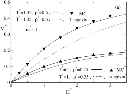
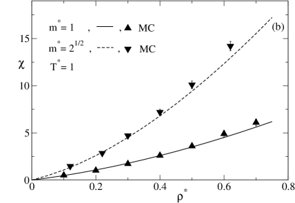
Figure 1: (a) Magnetization curves of DY fluids for different values of the reduced density $\rho^{*}$ and reduced temperature $T^{*}$ for $m^{*}=1$. (b) Magnetic zero-field susceptibility of DY fluids for different values of the reduced dipole moment and for the reduced temperature $T^{*}=1$. The symbols in both figures are the results of Monte Carlo simulations whereas the lines are obtained from the present DFT.

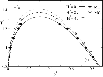
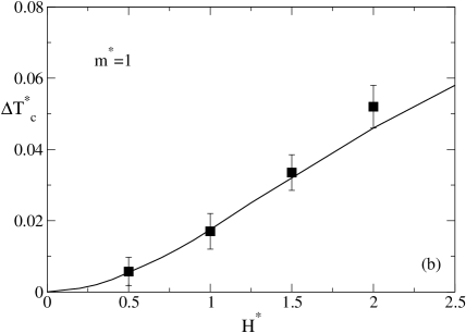
Figure 2: (a) Evolution of the phase diagram as function of the external magnetic field for a DY fluid in a needle-shaped container for $m^{*}=1$. (b) Shift of the critical temperature ($\Delta{T^{*}_{c}}=T^{*}_{c}(H)-T^{*}_{c}(0)$) of the liquid-vapor critical point as a function of the applied field for $m^{*}=1$. The symbols in both figures are the results of Monte Carlo simulations whereas the lines are obtained from the present DFT.

for a needle-shaped sample are displayed in Fig. 1(a) together with the result of the Langevin theory for $m^{*}=1$. Figure 1(a) shows that the interparticle interaction enhances the magnetization relative to the corresponding values of the Langevin theory. The theoretical data of the present theory are consistent with our new simulation data. For the reduced density $\rho^{*}=0.25$ we find both DFT and MC results to be in excellent, quantitative agreement for all field strengths. For $\rho^{*}=0.6$ the level of quantitative agreement reduces for larger field strengths.

The density dependence of the magnetic susceptibility obtained from the numerical solution of Eqs. (23) and (15) in comparison with earlier simulation data of Szalai et al [8] is displayed in Fig. 1(b). For the reduced dipole moment $m^{*}=1$ the agreement between the theoretical and simulation results is quite good, especially at lower densities. For $m^{*}=\sqrt{2}$ the level of quantitative agreement reduces for larger reduced densities.

The liquid-vapor phase diagrams at a given temperature $T$ follow from requiring the equality of the chemical potential and of the pressure for the densities of coexisting phases. The phase diagrams in the density-temperature plane are presented in Fig. 2(a) for various fixed values of the magnetic field and for the reduced dipole moment $m^{*}=1$. Figure 2(a) shows that for $H^{*}=0$ and $m^{*}=1$ there is no spontaneous magnetization within the framework of this theory, i.e., there is no ferromagnetic liquid phase. For $H^{*}\neq{0}$ there is a first-order phase transition between a low density gas and a high density liquid phase and both phases exhibit a nonzero magnetization. The agreement between the NpT+TP simulation and the DFT data is reasonable. For $m^{*}=1$ Fig. 2(b) represents the magnetic field dependence of the critical temperature corresponding to the liquid-gas phase transitions, obtained from the present DFT and liquid-gas equilibrium NpT+TP simulation data. For small $H^{*}$ both the theoretical and the simulation shifts increase quadratically as a function of the field strength. Similar results have been found for Stockmayer fluids in Refs. [17, 18].

6 Summary

The following main results have been obtained.

(1) Based on a second-order Taylor series expansion of the free energy functional of the dipolar Yukawa fluids, within the mean spherical approximation we have derived an analytical expression for the magnetization of ferrofluids. There is good agreement between the results of the density functional theory and the Monte Carlo simulation data for reduced dipole moments $m^{*}\lesssim 1.4$. The proposed implicit equation for the magnetization (Eq. (23)) extends the applicability of MSA for arbitrary strengths of the magnetic fields.

(2) We have derived analytical equations for the external field dependence of the pressure (Eq. (21)) and of the chemical potential (Eq. (19)) for dipolar Yukawa fluids which allows one to determine the magnetic field dependence of the liquid-vapor phase equilibria.

References

References

- [1] Buyevich Y A and Ivanov A O 1992 Physica A 190 276
- [2] Huke B and Lücke 2004 Rep. Prog. Phys. 67 1731
- [3] Russier V and Douzi M 1994 J. Colloid Interface Sci. 162 356
- [4] Groh B and Dietrich S 1994 Phys. Rev. E 50 3814
- [5] Szalai I and Dietrich S 2005 Mol. Phys. 103 2873
- [6] Range G M and Klapp S H L 2004 Phys. Rev. E 70 031201
- [7] Henderson D, Boda D, Chan K-Y and Szalai I 1999 J. Chem. Phys. 110 7348
- [8] Szalai I, Henderson D, Boda D and Chan K-Y 1999 J. Chem. Phys. 111 337
- [9] Wertheim M S 1971 J. Chem. Phys. 55 4291
- [10] Lebedev A V 1989 Magnetohydrodynamics 25 520
- [11] Morozov K I and Lebedev A V 1990 J. Magn. Magn. Mater. 85 51
- [12] Lovett R, Mou C Y and Buff F P 1976 J. Chem. Phys. 65 570
- [13] Hausleitner C Hafner J 1988 J. Phys. F: Met. Phys. 18 1013
- [14] Percus J K and Yevick G J 1956 Phys. Rev. 110 1
- [15] Tang Y 2003 J. Chem. Phys. 118 4141
- [16] Boda D, Liszi J and Szalai I 1995 Chem. Phys. Lett. 235 140
- [17] Groh B and Dietrich S 1996 Phys. Rev. E 53 2509
- [18] Boda D, Winkelmann J, Liszi J and Szalai I 1996 Mol. Phys. 87 601