Extreme Associated Functions: Optimally Linking Local Extremes to Large-scale Atmospheric Circulation Structures

Zusammenfassung

We present a new statistical method to optimally link local weather extremes to large-scale atmospheric circulation structures. The method is illustrated using July-August daily mean temperature at 2m height (T2m) time-series over the Netherlands and 500 hPa geopotential height (Z500) time-series over the Euroatlantic region of the ECMWF reanalysis dataset (ERA40). The method identifies patterns in the Z500 time-series that optimally describe, in a precise mathematical sense, the relationship with local warm extremes in the Netherlands. Two patterns are identified; the most important one corresponds to a blocking high pressure system leading to subsidence and calm, dry and sunny conditions over the Netherlands. The second one corresponds to a rare, easterly flow regime bringing warm, dry air into the region. The patterns are robust; they are also identified in shorter subsamples of the total dataset. The method is generally applicable and might prove useful in evaluating the performance of climate models in simulating local weather extremes.

Weather extremes such as extreme wind speeds, extreme precipitation or extreme warm or cold conditions are experienced locally. They are usually connected to circulation structures of much larger scale in the atmosphere. For example, if we restrict ourselves to the Netherlands, a well-known circulation structure that often leads to extreme hot summer days is a high pressure system that blocks the inflow of cooler maritime air masses. Moreover, the subsidence of air in its interior leads to clear skies and an abundance of sunshine that leads to high temperatures. If the blocking high persists and depletes the soil moisture due to lack of precipitation and increased evaporation, temperatures tend to soar, as it did in the European summer of 2003 Schär et al., (2004). Speculations about a positive feedback of dry soil on the persistence of the blocking high can also be found in the literature Ferranti and Viterbo, (2006).

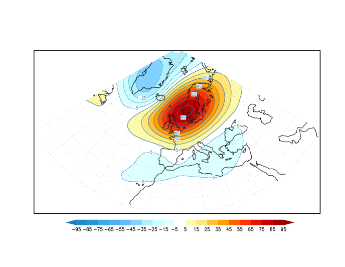
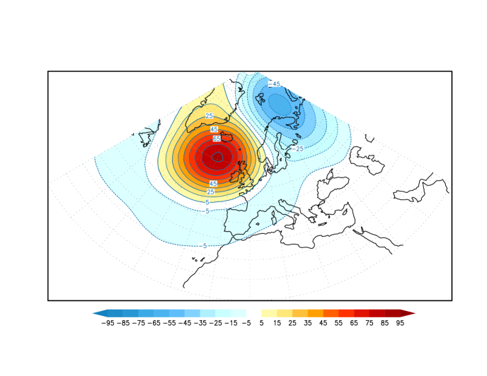
Abbildung 1: The leading two EOFs for the July and August Z500 daily anomaly field for 43 years of ERA-40 data (1958-2000). Left figure: first EOF; right figure: second EOF. Relative importances are $12.57\%$ and $11.79\%$ respectively. The patterns have been multiplied by one standard deviation of the corresponding amplitude time-series (in meters).

In order for climate models to correctly simulate the probability of extreme hot summer days, a crucial ingredient is the correct simulation of the probability of the occurrence of blocking. This is a well-known difficult feature of the atmospheric circulation to simulate realistically Pelly and Hoskins, (2003). The verification of models w.r.t. this aspect is, in practice, difficult as well, since idealized model experiments suggest a high degree of internal variability of blocking frequencies even on decadal timescales Liu and Opsteegh, (1995).

In a world with increasing concentrations of greenhouse gases, not only the temperature increases, also the large-scale circulation adjusts to achieve a new (thermo)dynamical balance. Models disagree on the magnitude and even the direction of this change locally van Ulden and van Oldenborgh, (2006). For instance, a change in the probability of European blocking conditions in summer immediately impacts the future probability of European heat waves. This makes probability estimates of future European heat waves very uncertain. To address the questions concerning the probability of future extreme weather events, and the evaluation of climate model simulations in this respect, it is necessary to have a descriptive method that links local weather extremes to large-scale circulation features. To the best of our knowledge, an optimal method to do so does not exist in the literature.

We identified two approaches in the literature to link local weather extremes to large-scale circulation features. In the first one, the circulation anomalies are classified first, the connection with local extremes is analyzed in second instance. The “Grosswetterlagen” developed by synoptic meteorologists for instance is one such classification Kysely, (2002). All kinds of clustering algorithms are another example Plaut and Simonnet, (2001); Cassou et al., (2005). In our opinion, this approach is not optimal since in the definition of the patterns, information about the extreme is not taken into account.

In the second approach, a measure of the local extreme does enter the definition of the large-scale circulation patterns. For instance, only atmospheric states are considered for which the local extreme occurs. Next a simple averaging operator is applied [“composite methodäs in Schaeffer et al., (2005)]or a clustering analysis is performed Sanchez-Gomez and Terray, (2005) . The composite method falls short since it finds by definition only one typical circulation anomaly and from synoptic experience we know that often different kind of circulation anomalies lead to a similar local weather extreme. The clustering analysis is debatable since the data record is often too short to identify clusters with enough statistical confidence Hsu and Zwiers, (2001).

The purpose of this paper is to report a new optimal method to relate local weather extremes to characteristic circulation patterns. This method objectively identifies, in a robust manner, the different circulation patterns that favor the occurrence of local weather extremes. The method is inspired by the Optimal Autocorrelation Functions of Selten et al., (1999). It is based on considering linear combinations of the dominant Empirical Orthogonal Functions that maximize a suitable statistical quantity. We illustrate our method by analyzing the statistical relation between extreme high daily mean temperatures at two meter height (T2m) in July and August in the Netherlands and the structure of the large-scale circulation as measured by the 500 hPa geopotential height field (Z500).

This paper is divided into five sections. Section 1 is focused on the data, where we explain the method to obtain the daily Z500 and T2m anomalies in Europe, and report the results of the EOF analysis of the Z500 anomaly data. In Sec. 2 we outline the procedure to optimize the quantity that describes the statistical relation between the Z500 and the extreme T2m anomalies, supported by the additional details in the Appendix. In Sec. 3 we identify the large-scale Z500 anomaly patterns that are associated with hot summer days in the Netherlands, demonstrate the robustness of our method and compare the patterns with patterns earlier reported in the literature. Finally we conclude this report in Sec. 7 with a discussion on the possible applications of our method.

1 The T2m and Z500 datasets, and EOF analysis of the Z500 data

Our data have been obtained from the ERA-40 reanalysis dataset, for the timespan Sept. 1957 to Aug. 2002, at 6 hourly intervals on a $2.5^{\circ}\times 2.5^{\circ}$ latitude-longitude grid. These data are publicly available at the ECMWF website $\mathsf{http://data.ecmwf.int/data/d/era40\_daily/}$. The T2m data over entire Europe, defined by $37.5^{\circ}$N-$70^{\circ}$N and $10^{\circ}$W-$40^{\circ}$E, and the Z500 data over $20^{\circ}$N-$90^{\circ}$N and $60^{\circ}$W-$60^{\circ}$E were downloaded. From these, the daily averages for T2m and Z500 fields for the years 1958-2000 (all together 43 years in total) were computed. This formed our full raw dataset.

In order to remove possible effects of global warming in the last decades of 20th century, detrending these fields prior to performing further calculations would be necessary. However, an analysis of the Z500 daily averaged field revealed no significant linear trend over these 43 years. Therefore the Z500 daily anomaly field was obtained by simply removing the seasonal cycle defined by an average over the entire period of 43 years. Greatbatch and Rong (2006) showed that over Europe, the trends in the ERA-40 reanalysis and NCEP-NCAR reanalysis are indeed small and similar.

A warming trend, however, is clearly present in the T2m field. For detrending the T2m field, the monthly averages for July and August were calculated from the daily averages at each gridpoint. Next, 11-year running means were computed for these monthly averaged T2m fields (for July and August separately), and that formed our baseline for calculating daily T2m anomaly field. This procedure does not yield the baseline for the first and the last 5 years (1958-1962 and 1996-2000); these were computed by extrapolating the baseline trend for the years 1963-1964 and 1995-1996 respectively.

For the EOF analysis of the Z500 anomaly field, note that most of the variance of atmospheric variability resides in the low-frequency part [10-90 day range Malone et al., (1984)]. Indeed, the dominant EOFs of Z500 anomaly fields proved insensitive to the application of 3-day, 5-day, 7-day, 9-day and 15-day running mean filters. For the sake of simplicity, therefore, we decided to only consider EOFs based on daily Z500 anomaly fields. The EOF analysis was performed on the regular lat-lon grid data with each grid point weighted by the cosine of its latitude to account for the different sizes of the grid cells. Using these weights, the EOFs $\mathbf{e}_{k}$ are orthogonal in space (note here that we use the same definition of vector dot product in space all throughout this paper)

$$\mathbf{e}_{k}\cdot\mathbf{e}_{l} \equiv$$ (1)

$$\frac{1}{\sum_{i=1}^{N}\cos(\phi_{i})}\sum_{i=1}^{N}e_{k}(\lambda_{i},\phi_{i})e_{l}(\lambda_{i},\phi_{i})\cos(\phi_{i})=\delta_{kl}\,,$$

where $\phi$ denotes latitude, $\lambda$ longitude and $N$ the total number of grid points, and $\delta_{kl}$ is the Kronecker delta. Each Z500 anomaly field can be expressed in terms of the EOFs as

$$\mathbf{Z500}(t)=\sum_{k=1}^{N}a_{k}(t)\mathbf{e}_{k}\,,$$ (2)

where the amplitudes $a_{k}$ are found by a projection of the Z500 anomaly on to the EOFs

$$a_{k}(t)=\mathbf{Z500}(t)\cdot\mathbf{e}_{k}\,.$$ (3)

A nice property of the EOFs is that their amplitude time-series are uncorrelated in time at zero lag

$$\left<a_{k}(t)a_{l}(t)\right>=\sigma_{k}^{2}\,\delta_{kl\,},$$ (4)

where the angular brackets $\langle.\rangle$ denote a time average and $\sigma_{k}^{2}$ denotes the eigenvalue of the $k$-th EOF which is equal to the variance of the corresponding amplitude time-series.

We found that July and August months produced very similar EOFs, while June and September EOFs were significantly different. We therefore decided to restrict the summer months to July and August. The leading two EOFs for the corresponding daily Z500 anomaly for 1958-2000 are shown in Fig. 1. The values correspond to one standard deviation of the corresponding amplitude. The two EOFs are not well separated (the eigenvalues are close together) and therefore we expect some mixing between the two patterns North et al., (1982). A linear combination of the two EOFs shifts the longitudinal position of the strong anomaly over Southern Scandinavia which is present in the first EOF. It resembles the summer NAO pattern as diagnosed by Greatbatch and Rong Greatbatch and Rong, (2006) (their figure 8).

2 Optimization procedure to establish the connection between Z500 anomalies and local extreme T2m

One of the first approaches we considered to establish the connection between Z500 daily anomaly fields and extreme daily T2m is the so-called “clustering method”, which identifies clusters of points in the vector space spanned by the dominant EOFs. The daily Z500 anomaly field for July and August over 43 years yields us precisely 2666 datapoints in this vector space. A projection of these daily anomalies on the two-dimensional vector space of the two leading EOFs (EOF1 and EOF2) is shown in Fig. 2. No clear clusters are apparent by simple visual inspection. One can imagine that defining clusters using existing cluster algorithms to identify clusters of points that correspond to specific large-scale circulation patterns that occur significantly more frequently than others is not a trivial undertaking. Often it turns out that using 40 years of data or so, the clusters identified are the result of sampling errors, due to too few data points Hsu and Zwiers, (2001); Berner and Branstator, (2007); Stephenson and O’Neill, (2004).

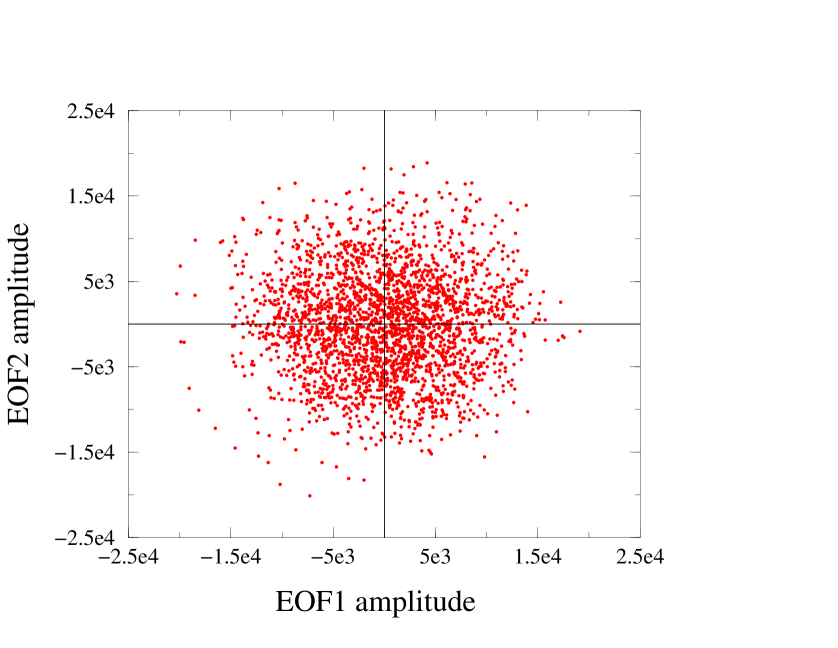
Abbildung 2: Projection of the daily Z500 anomaly field for July and August months for 43 years in the two-dimensional vector space spanned by the two leading EOFs.

Nevertheless, when we plot the T2m positive anomaly values at the center of the Netherlands ($52.5^{\circ}$N, $5^{\circ}$E) in a scatter plot with the amplitude of EOF1, a distinct “tiltïn the scatter plot emerges: i.e., with increasing amplitude of the leading EOF, the likelihood of having very hot summer days increases. Having inspected the same plots for the other EOFs we found a similar tilt for some of the other EOFs as well. From this point of view, finding the statistical relationship between T2m at a given place and the state of the large-scale atmospheric circulation can be reduced to a mathematical exercise that finds those linear combinations of EOFs that optimally bring out this tilt. In the remainder of this section, supported by the Appendix, we present a general, rigorous and robust procedure to achieve this.

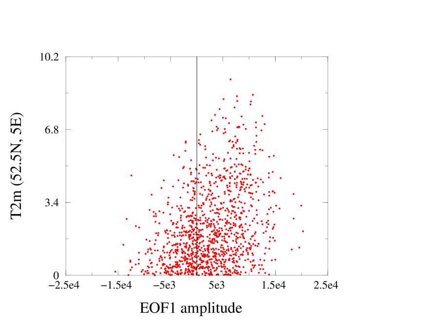
Abbildung 3: Scatter plot of T2m $\geq 0$ at the center of the Netherlands vs. the amplitude of leading Z500 EOF (EOF1). With increasing amplitude of the leading EOF, the likelihood of having very hot summer days increases.

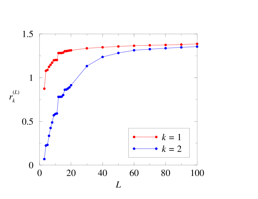
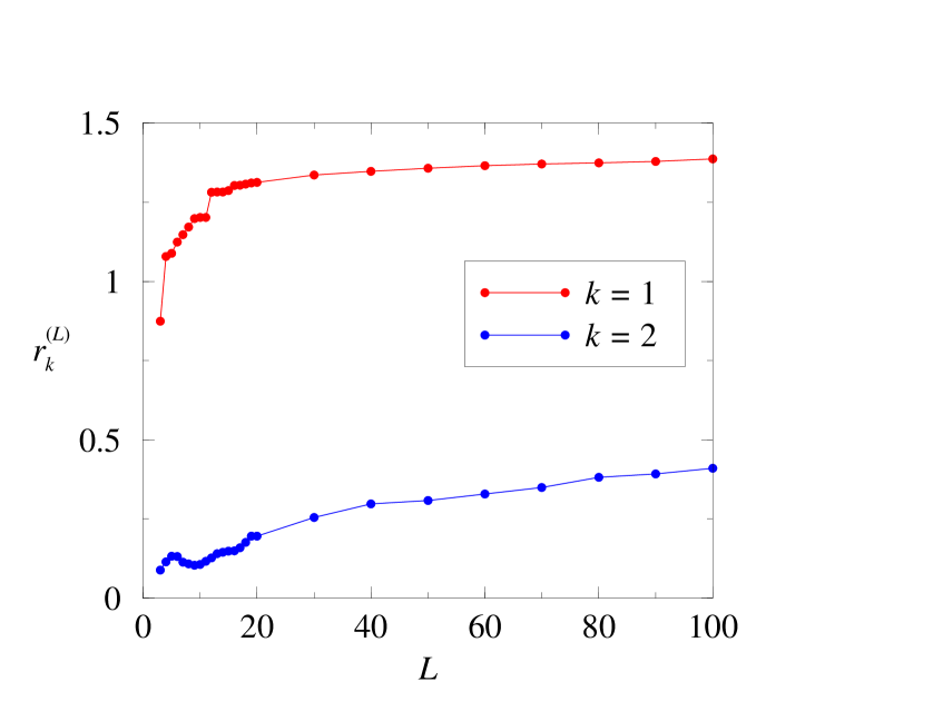
Abbildung 4: The behavior of $r$ as a function of $L$ for the first (red) and second (blue) EAFs. Left panel: patterns are orthogonal in space, but are correlated in time [option (a) in text]; right panel: patterns are uncorrelated in time but are not orthogonal in space [option (b) in text].

To represent this statistical relationship, we start by defining the following dimensionless quantity

$$r_{k}^{(L)}=\frac{\langle b_{k}^{(L)}(t)\,[T(t)]^{n}\rangle_{\mbox{\scriptsize p}}}{\langle\left[b_{k}^{(L)}(t)\right]^{2}\rangle^{\frac{1}{2}}_{\mbox{\scriptsize p}}\,\,\langle[T(t)]^{n}\rangle_{\mbox{\scriptsize p}}}.$$ (5)

Here the angular brackets $\langle.\rangle_{\mbox{\scriptsize p}}$ denotes a time average taken only over those days for which T2m$(t)\geq 0$, and $n$ is a positive number $>1$. The idea behind choosing $n>1$ is that for higher $T(t)$ it gives larger contribution to $r_{k}^{(L)}$: we are interested in high-temperature days at gridpoint $G$, we choose $n=2$ for this study. The variable $b_{k}^{(L)}(t)$ is the amplitude on day $t$ of a pattern, defined as a linear combination of the first $L$ EOFs. Since $L$ linear combinations can be defined that form a new complete basis in the subspace of the first $L$ EOFs we use the subscript $k$ to denote these different linear combinations.

We first concentrate on the calculation of the first pattern. Using $c^{(L)}_{j1}$ to denote the coefficients of this first linear combination then

$$b_{1}^{(L)}(t)=\sum_{j=1}^{L}c^{(L)}_{j1}\,a_{j}(t)\,.$$ (6)

Notice that since the time averages are taken only over those days for which T2m$(t)\geq 0$, $\langle b_{1}^{(L)}(t)\rangle_{\mbox{\scriptsize p}}\neq 0$, although $\langle b_{1}^{(L)}(t)\rangle=0$ since $\langle a_{j}(t)\rangle=0$.

Equations (5-6) imply that given the time-series of T2m and Z500 anomalies, the numerical value of $r^{(L)}_{1}$ depends only on $L$ and on the coefficients $c^{(L)}_{j1}$. For a given value of $L$, $c^{(L)}_{j1}$ are found by maximizing the square of $r^{(L)}_{1}$ within the vector space of the first $L$ EOFs (the square is taken since $r^{(L)}_{1}$ can take on negative values as well).

If we define for $T(t)\geq 0$,

$$\tilde{T}_{\mbox{\scriptsize p}}(t)=\frac{[T(t)]^{n}}{\langle[T(t)]^{n}\rangle_{\mbox{\scriptsize p}}}$$ (7)

then Eq. (5) can be rewritten for $k=1$ as

$$r^{(L)}_{1}=\frac{\langle b^{(L)}_{1}(t)\,\tilde{T}_{\mbox{\scriptsize p}}(t)\rangle_{\mbox{\scriptsize p}}}{\langle\left[b^{(L)}_{1}(t)\right]^{2}\rangle^{\frac{1}{2}}_{\mbox{\scriptsize p}}}.$$ (8)

In words, maximizing $\left[r^{(L)}_{1}\right]^{2}$ defines a pattern that for a change of one standard deviation in its amplitude $b_{1}$ brings about the largest change in the normalized positive temperature anomaly $\tilde{T}_{\mbox{\scriptsize p}}$ or put differently the local temperature responds most sensitively to changes in the normalized amplitude of this pattern. In this sense, the pattern is optimally linked to the local warm temperature extremes.

It is shown in the appendix that maximizing $\left[r^{(L)}_{1}\right]^{2}$ corresponds to the linear least squares fit of the EOF amplitude timeseries to $\tilde{T}_{\mbox{\scriptsize p}}(t)$

$$\tilde{T}^{(L)}_{\mbox{\scriptsize p}}(t)=\sum_{j=1}^{L}r^{(L)}_{1}c^{(L)}_{j1}\,a_{j}(t).$$ (9)

with the coefficients $c_{j1}$ given by

$$r^{(L)}_{1}c^{(L)}_{j1}=\sum_{i=1}^{L}\langle a_{i}(t)a_{j}(t)\rangle_{\mbox{\scriptsize p}}^{-1}\,\langle\tilde{T}_{\mbox{\scriptsize p}}(t)\,a_{i}(t)\rangle_{\mbox{\scriptsize p}}$$ (10)

This result makes sense since the linear least squares fit optimally combines the EOF amplitude timeseries to minimize the mean squared error between the actual temperature anomaly and the temperature anomaly estimated from the circulation anomaly at that day.

The procedure to find the remaining $(L-1)$ linear combinations is as follows. We first reduce the $Z500$ anomaly fields to the $(L-1)$ dimensional subspace $\mathbf{Z500}^{(L-1)}$ that is orthogonal to the first linear combination. In this subspace we again determine the linear combination that optimizes $r^{(L)}_{2}$. By construction, this value is lower than $r^{(L)}_{1}$. This procedure is repeated to determine all $L$ linear combinations with decreasing order of optimized values $r^{(L)}_{k}$.

There is no unique way to define the subspaces and how this is done affects the properties of the linear combinations. The linear combinations can either (a) be constructed to form an orthonormal basis in space, in which case their amplitudes are temporally correlated; or (b) they can be constructed so that the corresponding amplitudes are temporally uncorrelated, but in that case they are not orthonormal in space. In both cases, they form a complete basis in the space of the first $L$ EOFs

$$\mathbf{Z500}^{(L)}(t)=\sum_{k=1}^{L}b^{(L)}_{k}(t)\,\mathbf{f}^{(L)}_{k}\,.$$ (11)

We will call the patterns $\mathbf{f}^{(L)}_{k}$ Extreme Associated Functions (EAFs). The mathematical details on how to obtain $b^{(L)}_{k}(t)$ for both options can be found in the Appendix.

3 Statistical relationship between high summer temperature in the Netherlands and large-scale atmospheric circulation structures

We now need a criterion to determine the optimal number of EOFs in the linear combinations. The reason for limiting the number of EOFs in the linear combinations is apparent from Eq. (10). Here the inverse of the covariance matrix of the EOF amplitudes appears. This matrix becomes close to singular when low-variance EOFs are included in the linear combination. This makes the solution for the coefficients $c^{(L)}_{jk}$ ill-determined [see the general linear least squares section in Press et al., (1986) for a detailed discussion on this issue]. Typically what is observed is that the inclusion of many more low-variance EOFs only marginally improves the $r^{(L)}_{k}$ values, but that the corresponding patterns describe less variance and become “noisier” i.e. project onto Z500 variations at progressively smaller wavelengths. The optimal value of $L$ in a statistical procedure like this, denoted by $L_{c}$, is subjective, but nevertheless can be found from a tradeoff between the amount of variance that the patterns describe and their $r$-values.

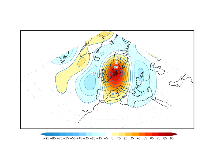
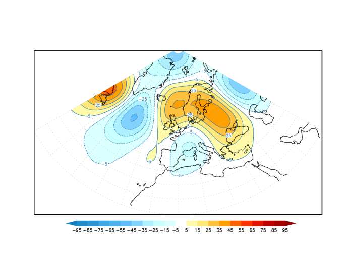
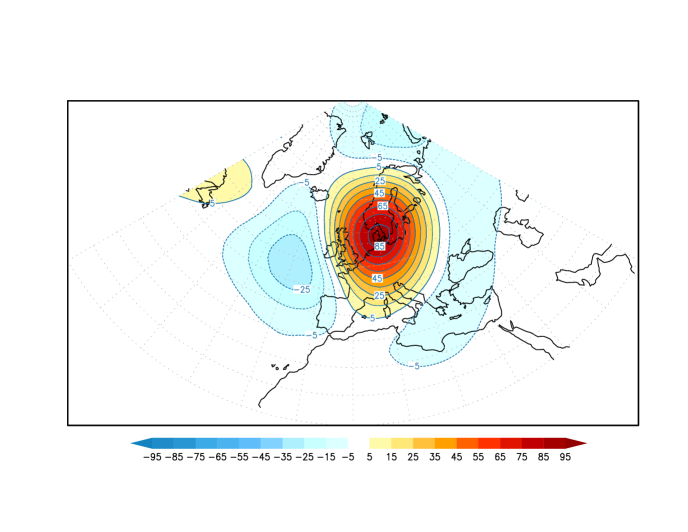
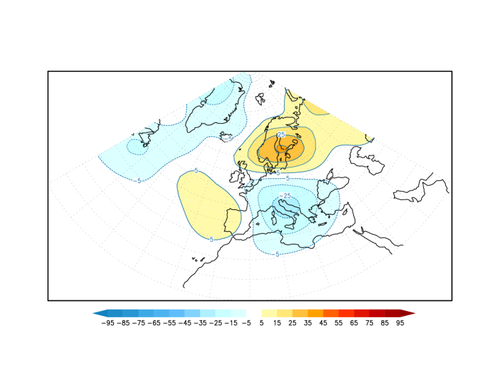
Abbildung 5: The leading two Z500 daily anomaly patterns (EAFs) that are associated with warm July and August daily temperatures in the Netherlands: EAFs orthogonal in space, corresponding to $L_{c}=12$ (top panel); EAF amplitudes uncorrelated in time, corresponding to $L_{c}=50$ (bottom panel). The first EAFs are shown on the left, and the second EAFs are shown on the right. All patterns have been multiplied by one standard deviation of the corresponding amplitude time-series (in meters).

The procedure to determine $L_{c}$ for the daily summer (July and August) temperature in the Netherlands [represented by T2m at ($52.5^{\circ}$N,$5^{\circ}$E)] and Z500 daily anomaly field over the region $20^{\circ}$N-$90^{\circ}$N and $60^{\circ}$W-$60^{\circ}$E for 43 years (1958-2000) is as follows. As can be expected, both $r^{(L)}_{1}$ and $r^{(L)}_{2}$ are increasing functions with $L$ [Fig. 4(left)] and the variance associated with the corresponding EAFs tends to decrease with increasing $L$ (not shown here). For option (a), both $r^{(L)}_{1}$ and $r^{(L)}_{2}$ improve significantly when including EOF12 in the linear combination; at the same time the variance of EAF1 decreases and the variance of EAF2 increases. Also the corresponding patterns change markedly. Between $L=12$ and $L=15$ the patterns, $r$-values and variances remain relatively unchanged. Beyond $L=15$ the $r$-values steadily increase, the variance decreases and the patterns become “noisier”. Simultaneously, the temporal correlation between the dominant two EAF patterns steadily increases with $L$. For large $L$, as Fig. 4(left) shows, both $r_{1}^{(L)}$ and $r_{2}^{(L)}$ values saturate to values very close to each other, and the solution tends to become degenerate. Our interpretation of this is that the information that is contained in the $Z500$ anomaly fields about the local temperatures in the Netherlands is shared among increasingly more patterns, which is an undesirable characteristic. For example, for $L=12$, the temporal correlation between EAF1 and EAF2 is $0.58$, for $L=50$ it is $0.93$. Based on these findings, we consider $L_{c}$ to be equal to $12$.

A similar graph for EAFs calculated following option (b) are also displayed in Fig. 4(right). By construction, the value of $r^{(L)}_{1}$ is the same. In this case, the variance decreases as well with increasing $L$, but much less so. The corresponding patterns are quite stable beyond $L=19$. It is only beyond $L=200$ or so that the second EAF more and more resembles the first EAF; for $L=19$ the spatial correlation between EAF1 and EAF2 is only 0.2 (they are almost orthogonal), for $L=200$ it is 0.4 and for $L=500$ it is 0.8. By construction, the temporal correlation between EAF1 and EAF2 remains zero. In this case, the choice of $L$ is not so critical and we simply choose $L_{c}=50$.

The results for the spatially orthogonal EAFs corresponding to $L_{c}=12$ and that for EAFs uncorrelated in time corresponding to $L_{c}=50$ are shown in Fig. 5. The first EAFs obtained from options (a) and (b) are very similar; the differences in the second are bigger. The first corresponds to a high pressure system, leading to clear skies over the Netherlands, an abundance of sunshine and a warm southeasterly flow. In addition to this circulation anomaly, the method finds another pattern that occurs less often; EAF2 corresponds to an easterly flow regime bringing warm dry continental air masses to the Netherlands. Option (b) gives a more localized $Z500$ anomaly pattern, with a warm, easterly flow into the Netherlands. Option (a) also captures the warm, easterly flow, but is less localized and is less well defined as a function of $L$. The $r^{(L)}_{2}$ value is larger for option (a), but it is temporally correlated to the first EAF. This implies that part of the information about the local warm temperatures in the Netherlands that is contained in the amplitude timeseries of EAF2 is already captured by EAF1; they are not independent. The $r^{(L)}_{2}$ value is smaller for option (b), but at least the information it contains about the local warm temperatures in the Netherlands is independent from EAF1. Given these considerations, we conclude option (b), constructing EAFs that are temporally uncorrelated is the best option.

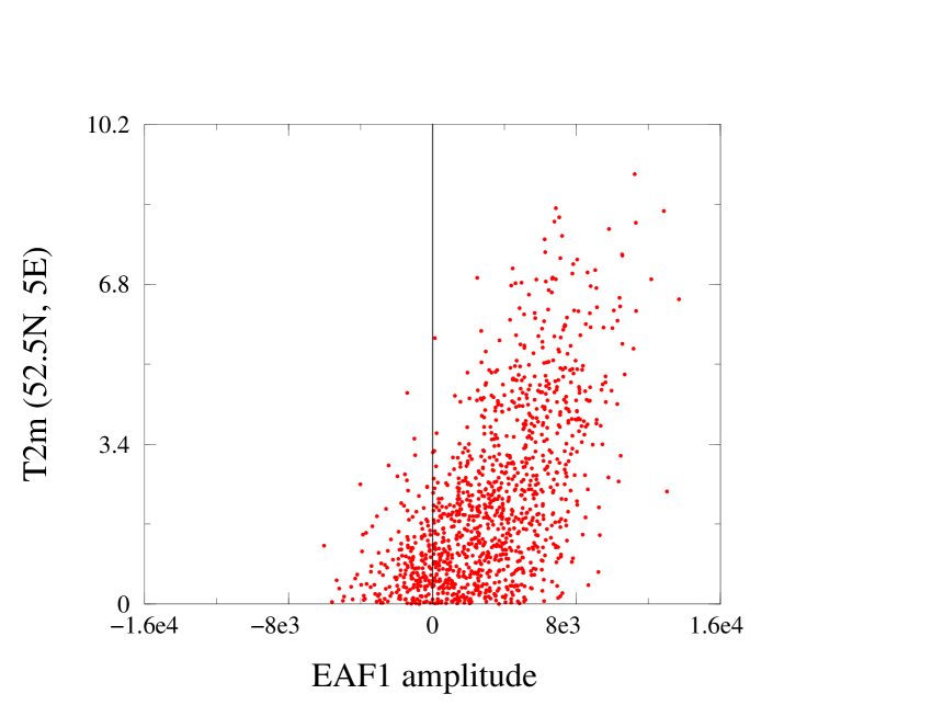
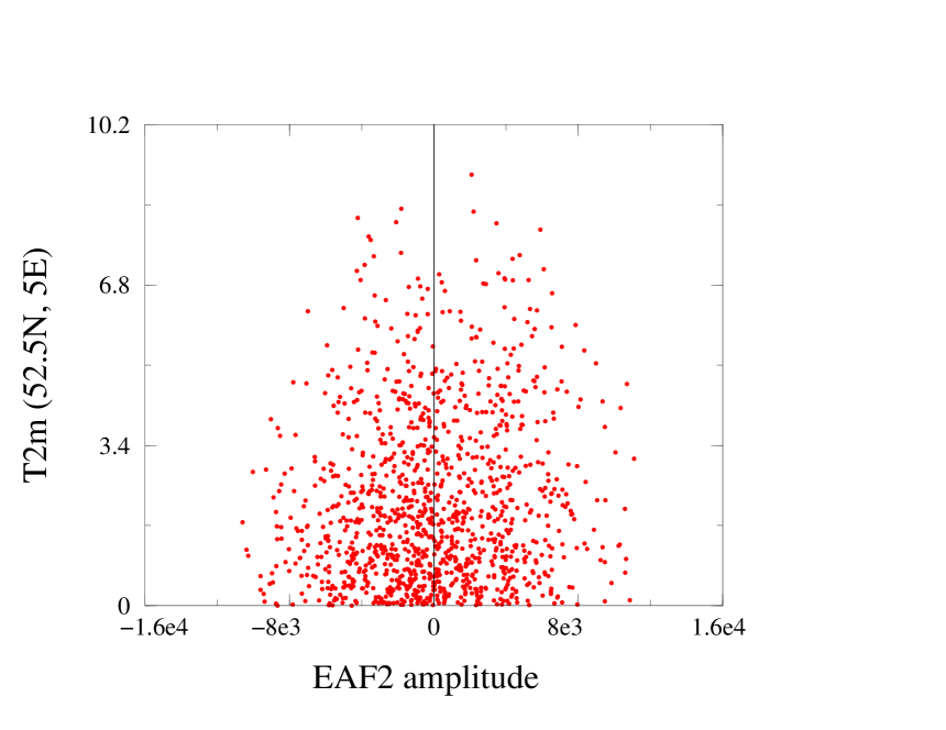
Abbildung 6: Scatter plots for the amplitudes of EAF1 (left) and EAF2 (right) that are uncorrelated in time, corresponding to $L_{c}=50$, against the daily mean two meter temperature in the Netherlands.

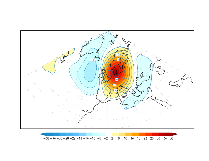
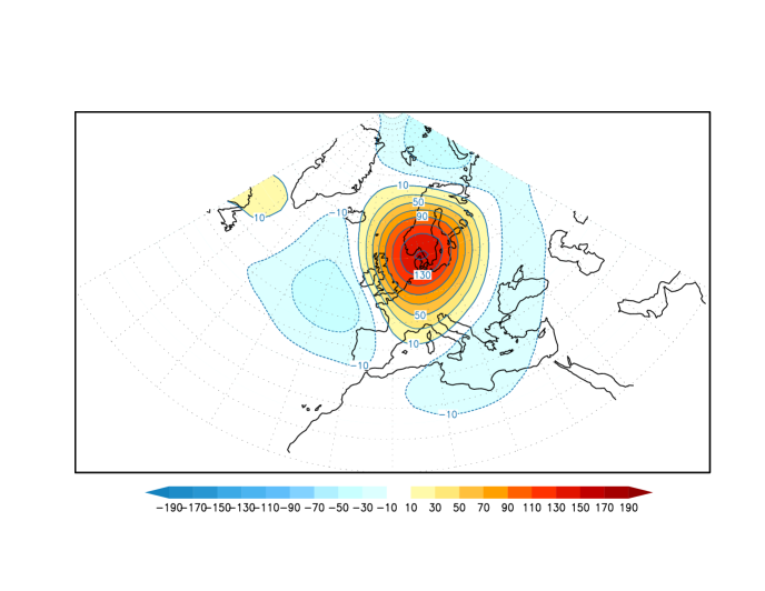
Abbildung 7: Daily Z500 anomaly field regressed on daily mean temperatures in The Netherlands in July and August in meters/Kelvin (left). Composite Z500 daily anomaly field for 5 warmest days in July and August in the Netherlands over the period 1958-2000 in meters.

The scatterplots of $b^{(L_{c}=50)}_{1}$ and $b^{(L_{c}=50)}_{2}$ against the positive temperature anomalies in the Netherlands for EAF1 and EAF2 that are uncorrelated in time are shown in Fig. 6. Compared to the EOF with the largest $r$ value (EOF1, see Fig. 3), the relationship of $b^{(L_{c}=50)}_{1}$ to temperature is much stronger. The $r$ value of the first EAF is almost a factor of 2 larger. The main contribution to the first EAF is from the first EOF, but also EOFs 3,4 and 6 contribute substantially. Only two EAFs are found with a clear connection (i.e., a tilt in the scatterplot) to warm extremes in the Netherlands. This information was spread mainly between EOFs 1, 3, 4 and 6. Regressing Z500 anomalies upon the temperature time-series in the Bilt gives a pattern that resembles EAF1 (Fig. 7). Also a simple compositing (averaging the 5 percent hottest days) yields a pattern very similar to EAF1 (Fig. 7). In addition to this, the EAF method is able to identify another, less dominant, flow configuration that leads to warm weather in the Netherlands through advection of warm airmasses from eastern Europe. Comparing EAF1 to the clusters of summer Z500 anomalies published in Cassou et al., (2005), we note that EAF1 is a combination of their ‘blocking’ and ‘Atlantic low’ regimes that favour warm conditions in all of France and Belgium (temperatures in the Netherlands were not analyzed). The easterly flow regime is not present in their clusters.

In order to check that this method to identify the relevant large-scale atmospheric circulation patterns for warm days in the Netherlands is robust, we have also performed the same analysis for the first 21 years (1958-1978) of daily summertime data and the last 21 years (1980-2000). In both cases we found very similar EAF1 patterns and corresponding scatter plots as for the full period. EAF2 however is only recovered in the second period. One interpretation of this is that EAF2 is less frequently present in the first period. As argued by Liu and Opsteegh, (1995) this variation could be entirely due to the chaotic nature of the atmospheric circulation and need not be caused by a factor external to the atmosphere (as for instance increasing levels of greenhouse gases, changes in sea surface temperatures or solar activity to name a few).

Instead of taking all positive temperature anomalies, a threshold could be introduced to Analise only the more extreme warm days. However, limiting the analysis to the 30% warmest positive temperature anomalies did not qualitatively change the first two EAFs. Also varying the value of the power applied to the temperature anomaly from 1 to 3, only quantitatively modified the resulting EAFs, but not qualitatively. A final test of robustness was that we limited the analysis to a smaller domain. Again we found the same two EAF patterns on a much smaller domain from 20 degrees east to 32.5 degrees west and 35 to 70 degrees north. The method thus produces robust patterns.

[Discussion: Applicability of the Extreme Associated Functions]

The Extreme Associated Function method developed in this study to establish the connection between local weather extremes and large-scale atmospheric circulation structures has several potentially useful applications.

First of all, since this method proved to satisfy several tests of rigor and robustness for the temperature extremes in the Netherlands, it can be applied for local temperature extremes at any other place, or for that matter for other forms of extreme local weather conditions as well, like precipitation or wind. In this sense the method is quite general.

EAFs can be used to evaluate the performance of climate models with respect to the occurrence of local weather extremes. The EAF method helps to answer the question whether the climate model is able to generate the same patterns that are found in nature to be responsible for local weather extremes with a similar probability of occurrence in an objective manner. In addition, to evaluate the impact of climate change on local weather extremes, the EAF method helps to answer the question whether the probability of certain local weather extremes changes in future scenario simulations due to a change in the probability of occurrence of the EAFs.

It might be found that some climate models are able to simulate the EAFs, but do not reproduce the local extremes well. Lenderink et al., (2007) for instance found that regional climate models forced with the right large-scale circulation structures at the domain boundaries nevertheless tended to overestimate the summer temperature variability in Europe due to deficiencies in the description of the hydrological cycle. The EAFs can be used to correct the model output for this discrepancy by applying the observed statistical relationship between the EAFs and the local extremes to the model generated EAFs.

By choosing the particular form of $r$ in Eq. (5) as the quantity to be optimized, the EAF method turns out to be equivalent to multiple linear regression. Other measures to describe the statistical relationship between circulation and temperature present in the scatterplot of Fig. 3 could be designed that would make the EAF method different from a multiple linear regression technique. In this sense, the EAF method is more general and potentially can be improved by designing a more apt measure.

Calculation of the EAFs by a repetitive maximization procedure

Since the entire appendix describes the procedure to calculate $b^{(L)}_{k}$, i.e., the $b_{k}$-values for a given $L$, we drop all superscripts involving $L$ for the sake of notational simplicity.

A.1. Calculation of the first EAF

To calculate which set of coefficients $c_{j1}$ maximize the value of $r_{1}^{2}$ as expressed in Eq. (8) we take the variation of $r_{1}^{2}$ w.r.t. variations $\delta c_{j1}$, and using Eq. (6), obtain

$$\delta r_{1}^{2}\,=\,2\times$$ (A.1.1)

$$\frac{\displaystyle{\sum_{l=1}^{L}\!\!\left\{\!\langle\tilde{T}(t)a_{k}(t)\rangle_{\mbox{\scriptsize p}}\langle\tilde{T}(t)a_{l}(t)\rangle_{\mbox{\scriptsize p}}\!-\![r_{1}^{\mbox{\scriptsize max}}]^{2}\!\langle a_{k}(t)a_{l}(t)\rangle_{\mbox{\scriptsize p}}\!\right\}\!c_{l1}\delta c_{k1}}}{\langle[b(t)]^{2}\rangle_{\mbox{\scriptsize p}}}$$

$$\hskip 76.82234pt\quad\mbox{for}\,\,k=1,\ldots,L\,.$$

This means that with the l.h.s. of Eq. (A.1.1) set to zero at the maximum of $r_{1}^{2}$ for any choice of $\delta c_{k1}$, we obtain a generalized eigenvalue equation: if we denote $\langle\tilde{T}(t)a_{k}(t)\rangle_{\mbox{\scriptsize p}}\langle\tilde{T}(t)a_{l}(t)\rangle_{\mbox{\scriptsize p}}$ by $\tilde{a}_{k}\,\tilde{a}_{l}$, and $\left[\langle a_{k}(t)a_{l}(t)\rangle_{\mbox{\scriptsize p}}\right]$ by $v^{2}_{kl}$ then Eq. (A.1.1) leads to

$$\sum_{l=1}^{L}\left\{\tilde{a}_{k}\,\tilde{a}_{l}\,-\,[r_{1}^{\mbox{\scriptsize max}}]^{2}\,v^{2}_{kl}\right\}\,c_{l1}\,=\,0\,.$$ (A.1.2)

Equation (A.1.2) can be written as a matrix equation

$$\mathbf{\tilde{A}}\,\mathbf{c}_{1}\,=[r_{1}^{\mbox{\scriptsize max}}]^{2}\,\mathbf{V}^{2}\,\mathbf{c}_{1},$$ (A.1.3)

where the $(k,l)$-th element of matrices $\mathbf{\tilde{A}}$ and $\mathbf{V}^{2}$ are given by $\tilde{a}_{k}\,\tilde{a}_{l}$ and $v^{2}_{kl}$ respectively, and the $l$-th element of the column vector $\mathbf{c}_{1}$ is given by $c_{l1}$. Note that in Eq. (A.1.2) $v^{2}_{kl}\not\propto\delta_{kl}$, since the time-average is defined only over the days for which T2m$(t)\geq 0$. Since matrix $\mathbf{\tilde{A}}$ is a tensor product of two column vectors $\mathbf{\tilde{A}}=\mathbf{\tilde{a}}\mathbf{\tilde{a}}^{\mbox{\scriptsize T}}$, where the superscript ‘T’ indicates transpose, the matrix equation (A.1.3) has only one eigenvector with non-zero eigenvalue, given by

$$\mathbf{c}_{1}\propto\mathbf{V}^{-2}\mathbf{a}.$$ (A.1.4)

or equivalently

$$c_{j1}\propto\sum_{i=1}^{L}\langle a_{i}(t)a_{j}(t)\rangle_{\mbox{\scriptsize p}}^{-1}\,\langle\tilde{T}_{\mbox{\scriptsize p}}(t)\,a_{i}(t)\rangle_{\mbox{\scriptsize p}}.$$ (A.1.5)

The corresponding optimized value $r_{1}$ is determined from Eq. (A.1.3).

The equivalence between the maximization of $r_{1}^{2}$ and the multiple linear regression of $\tilde{T}_{\mbox{\scriptsize p}}(t)$ on the timeseries of the EOF amplitudes $a_{k}(t)$’s [see Eq. (9)] is apparent by noticing that the above solution for $\mathbf{c}_{1}$ is the same as the solution of the multiple linear regression problem given in Eq. (10).

How the EAFs are determined from the coefficients $c_{jk}$ is shown in the next section in which we explain the calculation of the remaining $(L-1)$ EAFs.

A.2. Calculation of the remaining $(L-1)$ EAFs

As explained in the text, the calculation of the remaining $(L-1)$ linear combinations requires a choice between two options. (a) The patterns are orthogonal in space, or, (b) the amplitude timeseries are uncorrelated in time. We will show the implementation of both options.

We first discuss option (a).

Combining the expansion of $\mathbf{Z500}(t)$ into EOFs as in Eq. (2) and into EAFs as in Eq. (11) gives the following relation between the EOFs and EAFs

$$\mathbf{e}_{i}=\sum_{k=1}^{L}c_{ik}\,\mathbf{f}_{k}\,\,\,\,\,\mbox{for}\,\,i=1,\ldots,L$$ (A.2.1)

Option (a) demands the EAFs to be orthonormal in space which leads to the following condition for the corresponding coefficients $c_{jk}$ where we start from the orthonormality condition of the EOFs

$$\mathbf{e}_{i}\cdot\mathbf{e}_{j}=\sum_{k,l=1}^{L}c_{ik}\,c_{jl}\,\mathbf{f}_{k}\cdot\mathbf{f}_{l}=\sum_{k=1}^{L}c_{ik}\,c_{jk}=\delta_{ij}.$$ (A.2.2)

Additionally, it can be easily shown that

$$\sum_{i=1}^{L}c_{ik}\,c_{il}=\delta_{kl}.$$ (A.2.3)

Using Eq. (A.2.3), it is now straightforward to show from Eq. (A.2.1) that the EAFs can be calculated from the EOFs as

$$\mathbf{f}_{k}=\sum_{i=1}^{L}c_{ik}\,\mathbf{e}_{i}\,\,\,\,\mbox{for}\,\,k=1,\ldots,L.$$ (A.2.4)

Using this definition for the EAFs, the corresponding amplitudes $b_{k}(t)$ are found by

$$b_{k}(t)=\mathbf{f}_{k}\cdot\mathbf{Z500}(t).$$ (A.2.5)

We now discuss option (b).

For option (b), Eqs. (11) and (A.2.5) cannot hold simultaneously. To obtain the coefficients $c_{ij}$ for this option, we start with Eqs. (11) and define

$$b_{k}(t)=\sum_{i=1}^{L}c_{ik}\,a_{i}(t)=\sum_{i=1}^{L}c_{ik}\,\mathbf{e}_{k}\cdot\mathbf{Z500}(t)$$ (A.2.6)

$$\equiv\mathbf{g}_{k}\cdot\mathbf{Z500}(t)$$

Then the conditions that $b_{k}(t)$ and $b_{l}(t)$ are uncorrelated in time, i.e.,

$$\langle b_{k}(t)\,b_{l}(t)\rangle=\delta_{kl}$$ (A.2.7)

yields, using the fact that the EOF amplitudes are uncorrelated in time,

$$\sum_{i,j}^{L}c_{ik}\langle a_{i}(t)\,a_{j}(t)\rangle c_{jl}=\sum_{i}^{L}c_{ik}\,\sigma^{2}_{i}\,c_{il}=\delta_{kl}.$$ (A.2.8)

We then define

$$\mathbf{f}_{k}=\sum_{i=1}^{L}c_{ik}\,\sigma_{i}^{2}\,\mathbf{e}_{i}\,\,\,\,\mbox{for}\,\,k=1,\ldots,L$$ (A.2.9)

in terms of which Eq. (A.2.7) can be re-expressed as

$$\mathbf{f}_{k}\cdot\mathbf{g}_{l}=\delta_{kl}.$$ (A.2.10)

Note here that for option (a) the patterns $\mathbf{f}_{k}$ are automatically normalized to unity. For option (b), the patterns $\mathbf{f}_{k}$ can be normalized to one, but the normalization of $\mathbf{g}_{k}$ should be adjusted as well in order for Eq. (A.2.10) to remain valid.

To obtain the rest of the $(L-1)$ EAFs, the procedure described in Appendix A.1 needs to be repeated $L-1$ times, but certain care needs to be taken because of the orthonormality condition imposed by the definition of the set of EAFs. When these subtle issues are taken into account, the procedure becomes a repetition of the following three steps.

• Construct $\mathbf{Z500}^{\prime}(t)$, the Z500 daily anomaly field that lies within the vector subspace of the first $L$ EOFs but orthogonal to the first EAF. This is achieved in the following manner.

  First define

  $$\mathbf{e}^{\prime}_{j}=\mathbf{e}_{j}-(\mathbf{e}_{j}\cdot\mathbf{f}_{1})\,\mathbf{f}_{1}=\mathbf{e}_{j}-c_{j1}\,\mathbf{f}_{1}$$ (A.2.11)

  for $j=2,\ldots,L$. The dot product of both sides of Eq. (A.2.11) with $\mathbf{Z500}(t)$ then yields

  $$a^{\prime}_{j}(t)=a_{j}(t)-c_{j1}\,b_{1}(t)\quad\mbox{for}\,\,j=2,\ldots,L$$ (A.2.12)

  for option (a). For option (b), the corresponding expression is

  $$a^{\prime}_{j}(t)\!=a_{j}(t)-c_{j1}\,\sigma_{j}^{2}\,b_{1}(t)\,\mbox{for}\,\,j=2,\ldots,L.$$ (A.2.13)

• Calculate the coefficients $c^{\prime}_{j2}$ for $j=2,\ldots,L$ that maximize $r_{2}$.

  $$r_{2}c^{\prime}_{j2}=\sum_{i=1}^{L}\langle a^{\prime}_{i}(t)a^{\prime}_{j}(t)\rangle_{\mbox{\scriptsize p}}^{-1}\,\langle\tilde{T}_{\mbox{\scriptsize p}}(t)\,a^{\prime}_{i}(t)\rangle_{\mbox{\scriptsize p}}$$ (A.2.14)

  with

  $$b_{2}(t)=\sum_{j=2}^{L}c^{\prime}_{j2}\,a^{\prime}_{j}(t)\equiv\sum_{j=1}^{L}c_{j2}\,a_{2}(t).$$ (A.2.15)

• Next the coefficients $c_{j2}$ are calculated from the coefficients $c^{\prime}_{j2}$. For option (a) substitution of Eq. (A.2.12) into Eq. (A.2.15) leads to

  $$c_{j2}=c^{\prime}_{j2}-c_{j1}\,\sum_{i=1}^{L}\,c^{\prime}_{i2}\,c_{i1}\,\mbox{for}\,\,j=2,\ldots,L,$$ (A.2.16)

  with the convention that $c^{\prime}_{12}=0$. For option (b) substitution of Eq. (A.2.13) into Eq. (A.2.15) leads to

  $$c_{j2}\!=c^{\prime}_{j2}-c_{j1}\sum_{i=1}^{L}\!c^{\prime}_{i2}\,\sigma_{i}^{2}\,c_{i1}\,\mbox{for}\,\,j=2,\ldots,L,$$ (A.2.17)

  with the convention that $c^{\prime}_{12}=0$.

  These steps are to be repeated until all $L$ coefficient vectors have been determined. For option (a) the EAFs are then determined from Eq. (A.2.4), for option (b) from Eq. (A.2.9).