Crossover behavior in fluids with Coulomb interactions

Abstract

According to extensive experimental findings, the Ginzburg temperature $t_{G}$ for ionic fluids differs substantially from that of nonionic fluids [Schröer W., Weigärtner H. 2004 Pure Appl. Chem. 76 19]. A theoretical investigation of this outcome is proposed here by a mean field analysis of the interplay of short and long range interactions on the value of $t_{G}$. We consider a quite general continuous charge-asymmetric model made of charged hard spheres with additional short-range interactions (without electrostatic interactions the model belongs to the same universality class as the $3D$ Ising model). The effective Landau-Ginzburg Hamiltonian of the full system near its gas-liquid critical point is derived from which the Ginzburg temperature is calculated as a function of the ionicity. The results obtained in this way for $t_{G}$ are in good qualitative and sufficient quantitative agreement with available experimental data.

I Introduction

It is known that electrostatic forces determine the properties of various systems: physical as well as chemical or biological. In particular, the Coulomb interactions are of great importance when dealing with ionic fluids i.e., fluids consisting of dissociated cations and ions. In most cases the Coulomb interaction is the dominant interaction and due to its long-range character can substantially affect the critical properties and the phase behavior of ionic systems. Thus, the investigations concerning these issues are of great fundamental interest and practical importance.

Over the last ten years, both the phase diagrams and the critical behavior of ionic solutions have been intensively studied using both experimental and theoretical methods. These studies were stimulated by controversial experimental results, demonstrating the three types of the critical behavior in electrolytes solutions: (i) classical (or mean-field) and (ii) Ising-like behavior as well as (iii) crossover between the two singh_pitzer ; levelt1 ; pitzer ; gutkowski ; Schroer-04 ; Schroer:review . In accordance with these peculiarities, ionic solutions were conventionally divided into two classes, namely: “solvophobic” systems with Ising-like critical behavior in which Coulomb forces are not supposed to play a major role (the solvent is generally characterized by high dielectric constant) and “Coulombic” systems in which the phase separation is primarily driven by Coulomb interactions (the solvent is characterized by low dielectric constant). Hence the criticality of the Coulombic systems became a challenge for theory and experiment. A theoretical model which demonstrates the phase separation driven exclusively by Coulombic forces is a restricted primitive model (RPM) fisher1 ; stell1 . In this model the ionic fluid is described as an electroneutral binary mixture of charged hard spheres of equal diameter immersed in a structureless dielectric continuum. Early studies stillinger ; vorontsov ; stellwularsen established that the model has a gas-liquid phase transition. A reasonable theoretical description of the critical point in the RPM was accomplished at a mean-field (MF) level using integral equation methods stell1 ; stell3 and Debye-Hückel theory levinfisher . Due to controversial experimental findings, the critical behavior of the RPM has been under active debates fisher3 ; schroer ; Carvalho-Evans ; caillol1 ; valleau ; camp ; luijten1 ; caillol_mc ; patsahan_rpm ; Patsahan-Mryglod-Caillol-05 and strong evidence for an Ising universal class has been found by recent simulations caillol_mc ; luijten ; kim:04:0 and theoretical ciach:00:0 ; patsahan:04:1 ; ciach:05:0 ; ciach:06:1 studies.

In spite of significant progress in this field, the criticality of ionic systems are far from being completely understood. The investigation of more complex models is very important in understanding the nature of critical behavior of real ionic fluids demonstrating both the charge and size asymmetry as well as other complexities such as short-range attraction. A description of a crossover region when the critical point is approached is of particular interest for such models. Based on the experimental findings one can suggest that in ionic fluids the temperature interval of crossover regime, characterized by the Ginzburg temperature, is much smaller than observed in nonionic systems Schroer-04 . In particular, a sharp crossover was reported for the systems ${\rm Na-NH_{3}}$ Chieux-Sienko (see also Narayanan-Pitzer1 ; Narayanan-Pitzer2 ; Anisimov ). The analysis of experimental data for various ionic solutions confirmed that such systems generally exhibit crossover or, at least a tendency to crossover from the Ising behavior asymptotically close to the critical point, to the mean-field behavior upon increasing distance from the critical point Gutkowskii-Anisimov . Moreover, the systematic experimental investigations of the ionic systems such as tetra-$n$-butylammonium picrate, ${\rm Bu_{4}NPic}$, (for tetra-$n$-butylammonium picrate we will follow the notations from Schroer-04 ; Schroer:review ) in long chain $n$-alkanols with dielectric constant ranging from $3.6$ for $1$-tetradecanol to $16.8$ for $2$-propanol suggest an increasing tendency for crossover to the mean-field behavior when the Coulomb contribution becomes essential Schroer-04 ; Schroer:review ; Kleemeier . They also indicate that the ”Coulomb limit” reduced temperature of the RPM $T_{c}\simeq 0.05$ is valid for the almost non-polar long chain alkanols Schroer:review ; Kleemeier . It has been stressed Kleemeier that for solutions of ${\rm Bu_{4}NPic}$ in $1$-alkanols, the upper critical solution points are found to increase linearly with the chain length of the alcohols (that corresponds to the decrease of dielectric constant of the solvent). The experimental data for the critical points and the dielectric permittivities for solutions of ${\rm Bu_{4}NPic}$ in $1$-alkanols are given in Table 1 Kleemeier .

Table 1: The experimental parameters of the critical points (critical temperature $T_{c}$, critical mass fraction $w_{c}$) and the corresponding dielectric constants $\epsilon$ for solutions of ${\rm Bu_{4}NPic}$ in $1$-alkanols Kleemeier .

Solvent	$\epsilon(T_{c})$	$T_{c}/K$	$w_{c}$
$1$-oktanol	$9.5$	$298.55$	$0.336$
$1$-nonanol	$7.9$	$308.64$	$0.325$
$1$-decanol	$6.4$	$318.29$	$0.3152$
$1$-undecanol	$5.4$	$326.98$	$0.303$
$1$-dodecanol	$4.7$	$335.91$	$0.2951$
$1$-tridecanol	$4.3$	$342.35$	$0.284$
$1$-tetradecanol	$3.6$	$351.09$	$0.2721$

Theoretically the crossover behavior in ionic systems was firstly studied for the RPM fisher3 ; schroer ; Carvalho-Evans . The results obtained for the Ginzburg temperature were similar to those found for simple fluids in comparable fashion that is in variance to what is expected from the experiments Schroer-04 ; Schroer:review . Nearly at the same time in moreira-degama-fisher the crossover behavior of the lattice version of a fluid exhibiting the Ising behavior was studied as additional symmetrical electrostatic interactions were turned on. Based on the microscopic ground, the effective Hamiltonian in terms of the fluctuating field conjugate to the number density was derived in this work. Then, the crossover between the mean-field and Ising-like behavior was estimated using the Ginzburg criterion. The resulting crossover temperature calculated as function of the ionicity ${\cal I}$, which defines the strength of the Coulomb interaction relative to the short-range interaction, indicates its weak dependence but with the trends correlating with those observed experimentally.

In this paper we are also interested in the critical behavior of ionic fluids. In particular, we study the effect of the interplay of short-range and long-range interactions on the crossover behavior in such systems. We consider a continuous version of the charge-asymmetric ionic fluid in which both the long-range Coulomb and short-range van-der Waals-like interactions are included. Following moreira-degama-fisher we introduce the ionicity

$${\cal I}=\frac{1}{\beta^{*}}=\frac{|q_{1}q_{2}|}{k_{B}T\epsilon\sigma},$$ (1)

where $q_{i}$ is the charge on ion $i$, $k_{B}$ is the Boltzmann constant, $T$ is the temperature, $\sigma$ is collision diameter and $\epsilon$ is the dielectric constant. Then we derive the effective Hamiltonian of the charge-asymmetric model in the vicinity of the gas-liquid critical point. As in moreira-degama-fisher , the coefficients obtained for the effective Hamiltoninan have the forms of expansions in the ionicity but with new terms that appear in this case. Based on this Hamiltonian we estimate the Ginzburg temperatures as functions of the ionicity.

The layout of the paper is as follows. In Section 2 we introduce a continuous charge-asymmetric model with additional short-range attractive interactions included. We derive here the functional representation of the grand partition function of the model in terms of the fluctuating fields $\varphi_{\mathbf{k}}^{S}$ and $\varphi_{\mathbf{k}}^{D}$ conjugate to the total density and charge density, respectively. Section 3 is devoted to the derivation of the effective GLW Hamiltonian in the vicinity of the critical point. In Section 4 we calculate the Ginzburg temperature as a function of the ionicity for different values of the range of the attractive potential. We conclude in Section 5.

II Background

II.1 Model

Let us start with a general case of a classical charge-asymmetric two-component system consisting of $N$ particles among which there are $N_{1}$ particles of species $1$ and $N_{2}$ particles of species $2$. The pair interaction potential is assumed to be of the following form:

$$U_{\alpha\beta}(r)=\phi_{\alpha\beta}^{HS}(r)+\phi_{\alpha\beta}^{SR}(r)+\phi_{\alpha\beta}^{C}(r),$$ (2)

where $\phi_{\alpha\beta}^{HS}(r)$ is the interaction potential between the two additive hard spheres of diameters $\sigma_{\alpha}$ and $\sigma_{\beta}$. We call the two-component hard sphere system a reference system. Thermodynamic and structural properties of the reference system are assumed to be known. $\phi_{\alpha\beta}^{SR}(r)$ is the potential of the short-range (van-der-Waals-like ) attraction. $\phi_{\alpha\beta}^{C}(r)$ is the Coulomb potential: $\phi_{\alpha\beta}^{C}(r)=q_{\alpha}q_{\beta}\phi^{C}(r)/\epsilon$, where $\phi^{C}(r)=1/r$ and $\epsilon$ is the dielectric constant. The solution is made of both positive and negative ions so that the electroneutrality condition is satisfied,i.e. $\sum_{\alpha=1}^{2}q_{\alpha}c_{\alpha}=0$, where $c_{\alpha}$ is the concentration of the species $\alpha$, $c_{\alpha}=N_{\alpha}/N$. The ions of the species $\alpha=1$ are characterized by their hard sphere diameter $\sigma_{1}$ and their electrostatic charge $+q_{0}$ and those of species $\alpha=2$, characterized by diameter $\sigma_{2}$, bear opposite charge $-zq_{0}$ ($q_{0}$ is elementary charge and $z$ is the parameter of charge asymmetry). In general, the two-component system of hard spheres interacting via the potential $\phi_{\alpha\beta}^{SR}(r)$ can exhibit both the gas-liquid and demixion critical points which belong to the $3D$ Ising model universal class.

We consider the grand partition function (GPF) of the system which can be written as follows:

$$\Xi[\nu_{\alpha}]=\sum_{N_{1}\geq 0}\sum_{N_{2}\geq 0}\prod_{\alpha=1,2}\frac{\exp(\nu_{\alpha}N_{\alpha})}{N_{\alpha}!}\int({\rm d}\Gamma)\exp\left[-\frac{\beta}{2}\sum_{\alpha\beta}\sum_{ij}U_{\alpha\beta}(r_{ij})\right].$$ (3)

Here the following notations are used: $\nu_{\alpha}$ is the dimensionless chemical potential, $\nu_{\alpha}=\beta\mu_{\alpha}-3\ln\Lambda$, $\mu_{\alpha}$ is the chemical potential of the $\alpha$th species, $\beta$ is the reciprocal temperature, $\Lambda^{-1}=(2\pi m_{\alpha}\beta^{-1}/h^{2})^{1/2}$ is the inverse de Broglie thermal wavelength; $(\rm d\Gamma)$ is the element of configurational space of the particles: $(\rm d\Gamma)=\prod_{\alpha}\rm d\Gamma_{\alpha}$, $\rm d\Gamma_{\alpha}={\rm d}{\mathbf{r}}_{1}^{\alpha}{\rm d}{\mathbf{r}}_{2}^{\alpha}\ldots{\rm d}{\mathbf{r}}_{N_{\alpha}}^{\alpha}$.

Let us introduce the operators $\hat{\rho}_{{\mathbf{k}}}^{S}$ and $\hat{\rho}_{{\mathbf{k}}}^{D}$

$$\hat{\rho}_{{\mathbf{k}}}^{S}=\sum_{\alpha}\hat{\rho}_{{\mathbf{k}},\alpha}\qquad\hat{\rho}_{{\mathbf{k}}}^{D}=\sum_{\alpha}q_{\alpha}\hat{\rho}_{{\mathbf{k}},\alpha},$$

which are combinations of the Fourier transforms of the microscopic number density of the species $\alpha$: $\hat{\rho}_{{\mathbf{k}},\alpha}=\sum_{i}\exp(-{\rm i}{\mathbf{k}}{\mathbf{r}}_{i}^{\alpha})$. In this case the part of the Boltzmann factor entering eq. (3) which does not include hard sphere interactions can be presented as follows:

$$\exp\left[-\frac{\beta}{2}\sum_{\alpha\beta}\sum_{i,j}(U_{\alpha\beta}(r_{ij})-\phi_{\alpha\beta}^{HS}(r_{ij}))\right]=\exp\left[-\frac{\beta}{2V}\sum_{{\bf k}}(\tilde{\phi}_{SS}(k)\hat{\rho}_{{\mathbf{k}}}^{S}\hat{\rho}_{{\mathbf{-}k}}^{S}\right.$$

$$\left.+\tilde{\phi}_{DD}(k)\hat{\rho}_{{\mathbf{k}}}^{D}\hat{\rho}_{{\mathbf{-}k}}^{D}+2\tilde{\phi}_{SD}(k)\hat{\rho}_{{\mathbf{k}}}^{S}\hat{\rho}_{{\mathbf{-}k}}^{D})+\frac{\beta}{2V}\sum_{\alpha}N_{\alpha}\sum_{{\mathbf{k}}}(\tilde{\phi}_{\alpha\alpha}^{SR}(k)+q_{\alpha}^{2}\tilde{\phi}^{C}(k))\right],$$ (4)

where

$$\tilde{\phi}_{SS}(k) = \frac{1}{(1+z)^{2}}\left[z^{2}\tilde{\phi}_{11}^{SR}(k)+2z\tilde{\phi}_{12}^{SR}(k)+\tilde{\phi}_{22}^{SR}(k)\right]$$

$$\tilde{\phi}_{DD}(k) = \frac{1}{(1+z)^{2}}\left[\tilde{\phi}_{11}^{SR}(k)-2\tilde{\phi}_{12}^{SR}(k)+\tilde{\phi}_{22}^{SR}(k)\right]+\tilde{\phi}^{C}(k)$$

$$\tilde{\phi}_{SD}(k) = \frac{1}{(1+z)^{2}}\left[z\tilde{\phi}_{11}^{SR}(k)+(1-z)\tilde{\phi}_{12}^{SR}(k)-\tilde{\phi}_{22}^{SR}(k)\right]$$ (5)

with $\tilde{\phi}_{\alpha\beta}^{X\ldots}(k)$ being a Fourier transform of the corresponding interaction potential defined by

$$\tilde{\phi}_{\alpha\beta}^{X\ldots}(k)=\int_{V}\;{\rm d}{\mathbf{r}}{\phi}_{\alpha\beta}^{X\ldots}(r)\exp(-{\rm i}{\mathbf{k}}{\mathbf{r}}),\quad{\phi}_{\alpha\beta}^{X\ldots}(r)=\frac{1}{V}\sum_{\mathbf{k}}\tilde{\phi}_{\alpha\beta}^{X\ldots}(k)\exp({\rm i}{\mathbf{k}}{\mathbf{r}}).$$

Now we simplify our model assuming that

• The hard spheres will all be of the same diameter $\sigma_{\alpha}=\sigma$.

• $\widetilde{\phi}_{++}^{SR}(k)=\widetilde{\phi}_{--}^{SR}(k)=\widetilde{\phi}_{+-}^{SR}(k)=\widetilde{\phi}^{SR}(k)$.

With these restrictions the uncharged system can only exhibit a gas-liquid critical point and a possible demixion is ruled out.

Taking into account the assumptions mentioned above we thus have

$$\tilde{\phi}_{SS}(k)=\tilde{\phi}^{SR}(k)<0,\quad\tilde{\phi}_{DD}(k)=\tilde{\phi}^{C}(k)>0,\quad\tilde{\phi}_{SD}(k)\equiv 0.$$

Finally it will be convenient to introduce the effective range $b_{SR}$ of short-range interactions through the relations

$$\widetilde{\phi}^{SR}(k)=\widetilde{\phi}^{SR}(0)\left(1-\left(b_{SR}\;k\right)^{2}\right)+\mathcal{O}(k^{4})\;.$$ (6)

II.2 Functional representation of the grand partition function of an ionic model

Let us take advantage of the properties of Gaussian functional integrals to rewrite

$$\exp\left(\frac{1}{2}\sum_{\mathbf{k}}\widetilde{w}_{S}(k)\hat{\rho}_{{\mathbf{k}}}^{S}\hat{\rho}_{{\mathbf{-}k}}^{S}\right) = \frac{1}{{\cal N}_{w_{S}}}\int({\rm d}\varphi^{S})\exp\left(-\frac{1}{2}\sum_{\mathbf{k}}\left[\widetilde{w}_{S}(k)\right]^{-1}\varphi_{{\mathbf{k}}}^{S}\varphi_{{\mathbf{-}k}}^{S}\right.$$

$$\left.+\sum_{\mathbf{k}}\hat{\rho}_{{\mathbf{k}}}^{S}\varphi_{{\mathbf{k}}}^{S}\right),$$

$$\exp\left(-\frac{1}{2}\sum_{\mathbf{k}}\widetilde{w}_{C}(k)\hat{\rho}_{{\mathbf{k}}}^{D}\hat{\rho}_{{\mathbf{-}k}}^{D}\right) = \frac{1}{{\cal N}_{w_{C}}}\int({\rm d}\varphi^{D})\exp\left(-\frac{1}{2}\sum_{\mathbf{k}}\left[\widetilde{w}_{C}(k)\right]^{-1}\varphi_{{\mathbf{k}}}^{D}\varphi_{{\mathbf{-}k}}^{D}\right.$$

$$\left.+{\rm i}\sum_{\mathbf{k}}\hat{\rho}_{{\mathbf{k}}}^{D}\varphi_{{\mathbf{k}}}^{D}\right),$$

with

$${\cal N}_{w_{S}}=\int({\rm d}\varphi^{S})\exp\left(-\frac{1}{2}\sum_{\mathbf{k}}\left[\widetilde{w}_{S}(k)\right]^{-1}\varphi_{{\mathbf{k}}}^{S}\varphi_{{\mathbf{-}k}}^{S}\right)$$

$${\cal N}_{w_{C}}=\int({\rm d}\varphi^{D})\exp\left(-\frac{1}{2}\sum_{\mathbf{k}}\left[\widetilde{w}_{C}(k)\right]^{-1}\varphi_{{\mathbf{k}}}^{D}\varphi_{{\mathbf{-}k}}^{D}\right).$$

and

$$({\rm d}\varphi^{A})=\prod_{{\mathbf{k}}}^{\prime}{\rm d}\varphi_{{\mathbf{k}}}^{A}=\prod_{{\mathbf{k}}}^{\prime}{\rm d}(\Re\varphi_{{\mathbf{k}}}^{A}){\rm d}(\Im\varphi_{{\mathbf{k}}}^{A}),\qquad A=S,D.$$

In the above equations we also introduced the notations $\widetilde{w}_{S}(k)=-\beta\widetilde{\phi}_{SS}(k)/V$ and $\widetilde{w}_{C}(k)=\widetilde{\phi}^{C}(k)/V$.

As a result, we can rewrite $\Xi[\nu_{\alpha}]$ in the form of a functional integral

$$\Xi[\nu_{\alpha}]=\frac{1}{{\cal N}_{w_{S}}}\frac{1}{{\cal N}_{w_{C}}}\int({\rm d}\varphi^{S})({\rm d}\varphi^{D})\exp\left(-{\cal H}[\nu_{\alpha},\varphi^{S},\varphi^{D}]\right),$$ (7)

where the action ${\cal H}$ reads as

$${\cal H}[\nu_{\alpha},\varphi^{S},\varphi^{D}] = \frac{1}{2}\sum_{\mathbf{k}}\left[\widetilde{w}_{S}(k)\right]^{-1}\varphi_{{\mathbf{k}}}^{S}\varphi_{-{\mathbf{k}}}^{S}+\frac{1}{2}\sum_{\mathbf{k}}\left[\widetilde{w}_{C}(k)\right]^{-1}\varphi_{{\mathbf{k}}}^{D}\varphi_{-{\mathbf{k}}}^{D}$$ (8)

$$-\ln\Xi_{HS}[\overline{\nu}_{S}+\varphi^{S},\overline{\nu}_{D}+{\rm i}\beta^{1/2}\varphi^{D}],$$

$$\overline{\nu}_{S}=\frac{z}{1+z}\bar{\nu}_{1}+\frac{1}{1+z}\bar{\nu}_{2},\qquad\bar{\nu}_{D}=\frac{1}{q_{0}(1+z)}(\bar{\nu}_{1}-\bar{\nu}_{2}).$$ (9)

where the ”renormalized” chemical potentials $\overline{\nu}_{\alpha}$ are defined as

$$\overline{\nu_{\alpha}}=\nu_{\alpha}+\frac{1}{2}\sum_{\mathbf{k}}\left(-\widetilde{w}_{S}(k)+\beta q_{\alpha}^{2}\widetilde{w}_{C}(k)\right),\qquad\alpha=1,2.$$ (10)

Let us define $\Delta\nu^{S}=\overline{\nu}_{S}-\varphi_{0}^{S}$ and $\widetilde{\varphi}_{\mathbf{k}}^{S}=\Delta\nu^{S}+\varphi_{\mathbf{k}}^{S}$ with $\varphi_{0}^{S}$ chosen as the chemical potential of the hard spheres. This leads to the relation

$$\overline{\nu}_{S}+\varphi^{S}=\varphi_{0}^{S}+\widetilde{\varphi}^{S}.$$ (11)

Now we present $\ln\Xi_{HS}[\ldots]$ in the form of a cumulant expansion

$$\ln\Xi_{HS}[\ldots] = \sum_{n\geq 0}\frac{1}{n!}\sum_{i_{n}\geq 1}\sum_{{\mathbf{k}}_{1},\ldots,{\mathbf{k}}_{n}}{\mathfrak{M}}_{n}^{(i_{n})}[\varphi_{0}^{S},\overline{\nu}_{D};k_{1},\ldots,k_{n}]\widetilde{\varphi}_{{\bf{k}}_{1}}^{D}\ldots\widetilde{\varphi}_{{\bf{k}}_{i_{n}}}^{D}$$ (12)

$$\widetilde{\varphi}_{{\bf{k}}_{i_{n+1}}}^{S}\ldots\widetilde{\varphi}_{{\bf{k}}_{n}}^{S}\delta_{{\bf{k}}_{1}+\ldots+{\bf{k}}_{n}},$$

where ${\mathfrak{M}}_{n}^{(i_{n})}[\varphi_{0}^{S},\overline{\nu}_{D};k_{1},\ldots,k_{n}]$ is the $n$th cumulant (or the $n$th order truncated correlation function) defined by

$${\mathfrak{M}}_{n}^{(i_{n})}[\varphi_{0}^{S},\overline{\nu}_{D};k_{1},\ldots,k_{n}]=\frac{\partial^{n}\ln\Xi_{HS}[\ldots]}{\partial\widetilde{\varphi}_{{\bf{k}}_{1}}^{D}\ldots\partial\widetilde{\varphi}_{{\bf{k}}_{i_{n}}}^{D}\partial\widetilde{\varphi}_{{\bf{k}}_{i_{n+1}}}^{S}\ldots\partial\widetilde{\varphi}_{{\bf{k}}_{n}}^{S}}|_{\varphi_{0}^{S},\overline{\nu}_{D}}.$$ (13)

In particular it follows from (13) that

$${\mathfrak{M}}_{0}^{(0)}=\ln\Xi_{HS}[\varphi_{0}^{S},\overline{\nu}_{D}].$$ (14)

The expressions for the cumulants of higher order (for $i_{n}\leq 4$) are given in Appendix A. It should be noted that, contrary to moreira-degama-fisher , (12) includes all powers (even and odd) of the field $\varphi_{{\mathbf{k}}}^{S}$ conjugate to the total number density. It should be clear that the coefficients in the cumulant expansion (12) depend on the chemical potential (or, equivalently, on the density).

III Effective Hamiltonian in the vicinity of the critical point

Taking into account (12) we can rewrite (7)-(8) as follows

$$\Xi[\nu_{\alpha}] = \frac{1}{{\cal N}_{w_{S}}}\exp\left(-\overline{\cal H}\right)\int({\rm d}\widetilde{\varphi}^{S})\exp\left(-\frac{1}{2}\sum_{\mathbf{k}}\left[\widetilde{w}_{S}(k)\right]^{-1}\widetilde{\varphi}_{{\mathbf{k}}}^{S}\widetilde{\varphi}_{-{\mathbf{k}}}^{S}\right.$$ (15)

$$\left.+\left[\widetilde{w}_{S}(0)\right]^{-1}\Delta\nu^{S}\widetilde{\varphi}_{0}^{S}+\sum_{n\geq 1}\frac{1}{n!}\sum_{{\mathbf{k}}_{1},\ldots,{\mathbf{k}}_{n}}{\mathfrak{M}}_{n}^{(0)}[\varphi_{0}^{S},\overline{\nu}_{D}]\widetilde{\varphi}_{{\bf{k}}_{1}}^{S}\ldots\widetilde{\varphi}_{{\bf{k}}_{n}}^{S}\right.$$

$$\left.\times\delta_{{\bf{k}}_{1}+\ldots+{\bf{k}}_{n}}\right){\cal V}[\widetilde{\varphi}_{{\bf{k}}}^{S}],$$

where

$$\overline{\cal H}=\frac{1}{2}\left[\widetilde{w}_{S}(0)\right]^{-1}(\Delta\nu^{S})^{2}-\ln\Xi_{HS}[\varphi_{0}^{S}],$$

$${\cal V}[\widetilde{\varphi}_{{\bf{k}}}^{S}] = \frac{1}{{\cal N}_{w_{C}}}\int({\rm d}\widetilde{\varphi}^{D})\exp\left(-\frac{1}{2}\sum_{\mathbf{k}}\left[\widetilde{w}_{C}(k)\right]^{-1}\widetilde{\varphi}_{{\mathbf{k}}}^{D}\widetilde{\varphi}_{-{\mathbf{k}}}^{D}+\frac{1}{2}\sum_{\mathbf{k}}{\mathfrak{M}}_{2}^{(2)}\widetilde{\varphi}_{{\mathbf{k}}}^{D}\widetilde{\varphi}_{-{\mathbf{k}}}^{D}\right.$$ (16)

$$\left.+\frac{1}{2}\sum_{\mathbf{k}_{1},\mathbf{k}_{2},\mathbf{k}_{3}}{\mathfrak{M}}_{3}^{(2)}\widetilde{\varphi}_{{\mathbf{k}}_{1}}^{D}\widetilde{\varphi}_{{\mathbf{k}}_{2}}^{D}\widetilde{\varphi}_{{\mathbf{k}}_{3}}^{S}\delta_{{\bf{k}}_{1}+{\bf{k}}_{2}+{\bf{k}}_{3}}+\frac{1}{4}\sum_{\mathbf{k}_{1},\ldots,\mathbf{k}_{4}}{\mathfrak{M}}_{4}^{(2)}\widetilde{\varphi}_{{\mathbf{k}}_{1}}^{D}\widetilde{\varphi}_{{\mathbf{k}}_{2}}^{D}\widetilde{\varphi}_{{\mathbf{k}}_{3}}^{S}\right.$$

$$\left.\times\widetilde{\varphi}_{{\mathbf{k}}_{4}}^{S}\delta_{{\bf{k}}_{1}+\ldots+{\bf{k}}_{4}}+\frac{1}{6}\sum_{\mathbf{k}_{1},\ldots,\mathbf{k}_{4}}{\mathfrak{M}}_{4}^{(3)}\widetilde{\varphi}_{{\mathbf{k}}_{1}}^{D}\widetilde{\varphi}_{{\mathbf{k}}_{2}}^{D}\widetilde{\varphi}_{{\mathbf{k}}_{3}}^{D}\widetilde{\varphi}_{{\mathbf{k}}_{4}}^{S}\delta_{{\bf{k}}_{1}+\ldots+{\bf{k}}_{4}}+\ldots\right).$$

It is worth noting here that unlike to the case considered in moreira-degama-fisher we obtain in (16) terms proportional to $\left(\widetilde{\varphi}^{S}\right)^{2}\left(\widetilde{\varphi}^{D}\right)^{2}$ and $\widetilde{\varphi}^{S}\left(\widetilde{\varphi}^{D}\right)^{3}$. While the former is connected with an absence of a lattice symmetry, the the latter stems from charge asymmetry.

Our aim now is to derive the effective Landau-Ginzburg (LG) Hamiltonian. Since we are interested in the gas-liquid critical point, this Hamiltonian should be written in terms of fields $\widetilde{\varphi}_{{\bf{k}}}^{S}$ conjugate to the fluctuation modes of the total number density.

To this end we integrate out $\widetilde{\varphi}_{{\bf{k}}}^{D}$ in (16) using a Gaussian measure. As a result, we can present ${\cal V}[\widetilde{\varphi}_{{\bf{k}}}^{S}]$ as follows:

$${\cal V}[\delta\widetilde{\varphi}_{{\bf{k}}}^{S}] = \frac{{\cal N}_{W_{C}}}{{\cal N}_{w_{C}}}\left[1+\langle{\cal A}\rangle_{G}+\frac{1}{2!}\langle{\cal A}^{2}\rangle_{G}+\frac{1}{3!}\langle{\cal A}^{3}\rangle_{G}+\ldots\right],$$ (17)

where $\langle\ldots\rangle_{G}$ means

$$\langle\ldots\rangle_{G}=\frac{1}{{\cal N}_{W_{C}}}\int({\rm d}\varphi^{D})\;\ldots\exp\left(-\frac{1}{2}\sum_{\mathbf{k}}\widetilde{W}_{C}(k)\varphi_{{\mathbf{k}}}^{D}\varphi_{-{\mathbf{k}}}^{D}\right)$$

with $\widetilde{W}_{C}(k)$ given by

$$\widetilde{W}_{C}(k)=\left[\widetilde{w}_{C}(k)\right]^{-1}+y^{2}{\widetilde{G}}_{1}$$ (18)

and $y^{2}$ being the ionicity introduced by (1): $y^{2}={\cal I}$

Taking into account (1) and the recurrence formulas of Appendix A ${\cal A}$ may be written as a formal expansion in terms of $y^{2}$

$${\cal A} = -\frac{y^{2}}{2}\sum_{\mathbf{k}_{1},\mathbf{k}_{2},\mathbf{k}_{3}}{\widetilde{G}}_{2}(k_{1},k_{2}+k_{3})\varphi_{{\mathbf{k}}_{1}}^{D}\varphi_{{\mathbf{k}}_{2}}^{D}\varphi_{{\mathbf{k}}_{3}}^{S}\delta_{{\bf{k}}_{1}+{\bf{k}}_{2}+{\bf{k}}_{3}}-\frac{y^{2}}{4}\sum_{\mathbf{k}_{1},\ldots,\mathbf{k}_{4}}{\widetilde{G}}_{3}(k_{1},k_{2},k_{3}+k_{4})$$ (19)

$$\times\varphi_{{\mathbf{k}}_{1}}^{D}\varphi_{{\mathbf{k}}_{2}}^{D}\varphi_{{\mathbf{k}}_{3}}^{S}\varphi_{{\mathbf{k}}_{4}}^{S}\delta_{{\bf{k}}_{1}+\ldots+{\bf{k}}_{4}}-\frac{{\rm i}y^{3}}{6}\frac{(1-z)}{\sqrt{z}}\sum_{\mathbf{k}_{1},\ldots,\mathbf{k}_{4}}{\widetilde{G}}_{2}(k_{1},k_{2}+k_{3}+k_{4})$$

$$\times\varphi_{{\mathbf{k}}_{1}}^{D}\varphi_{{\mathbf{k}}_{2}}^{D}\varphi_{{\mathbf{k}}_{3}}^{D}\varphi_{{\mathbf{k}}_{4}}^{S}\delta_{{\bf{k}}_{1}+\ldots+{\bf{k}}_{4}}+\ldots.$$

In (18)-(19) the “tilde” over $\varphi_{{\mathbf{k}}}^{D(S)}$ was omitted for the sake of simplicity.

It should be mentioned that the dependence of ${\widetilde{G}}_{n}(k_{1},k_{2},\ldots,k_{n})$ on the $k_{i}$ is very complicated. Since we consider here the behavior of the system near the critical point the limiting case of $k_{i}=0$ is of particular interest. Therefore, we substitute in (17)

$${\widetilde{G}}_{n}(k_{1},k_{2},\ldots,k_{n})\equiv{\widetilde{G}}_{n}(0,\ldots)\qquad n\geq 3$$

and

$${\widetilde{G}}_{2}(k)={\widetilde{G}}_{2}(0)(1+g^{2}k^{2}),$$ (20)

with

$$g^{2}=\frac{\widetilde{G}_{22}(0)}{2\widetilde{G}_{2}(0)},\qquad\widetilde{G}_{22}(0)=\frac{\partial^{2}\widetilde{G}_{2}(k)}{\partial k^{2}}|_{k=0}.$$ (21)

Having integrated out eq. (17) $\Xi[\nu_{\alpha}]$ takes the form:

$$\Xi[\nu_{\alpha}]=\frac{1}{{\cal N}_{w_{S}}}\prod_{{\mathbf{k}}}\left(1+y^{2}\langle N\rangle_{HS}\widetilde{w}_{C}(k)\right)^{-1}\int\;({\rm d}\varphi^{S})\exp\left(-{\cal H}^{eff}[\varphi^{S}]\right),$$

$${\cal H}^{eff}[\varphi^{S}]=-\sum_{n\geq 0}\frac{1}{n!}\sum_{{\mathbf{k}}_{1},\ldots,{\mathbf{k}}_{n}}a_{n}\widetilde{\varphi}_{{\bf{k}}_{1}}^{S}\ldots\widetilde{\varphi}_{{\bf{k}}_{n}}^{S}\delta_{{\bf{k}}_{1}+\ldots+{\bf{k}}_{n}},$$ (22)

where we have for the coefficients $a_{n}$

$$a_{0} = -\overline{\cal H},$$ (23)

$$a_{1} = \langle N\rangle_{HS}+[\widetilde{w}_{S}(0)]^{-1}\Delta\nu^{S}-\frac{y^{2}}{2}\widetilde{G}_{2}(0)\sum_{{\mathbf{q}}}\widetilde{\Delta}(q)+\frac{y^{4}}{8}\left(3\widetilde{G}_{3}(0)+\frac{(1-z)^{2}-2z}{z}\right.$$ (24)

$$\left.\times\widetilde{G}_{2}(0)\right)\left[\sum_{{\mathbf{q}}}\widetilde{\Delta}(q)\right]^{2},$$

$$a_{2} = -[\widetilde{w}_{S}(k)]^{-1}+\widetilde{G}_{2}(k)-\frac{y^{2}}{2}\widetilde{G}_{3}(0)\sum_{{\mathbf{q}}}\widetilde{\Delta}(q)+\frac{y^{4}}{2}[\widetilde{G}_{2}(0)]^{2}\sum_{{\mathbf{q}}}\widetilde{\Delta}(q)\widetilde{\Delta}(\mid{\mathbf{k}}+{\mathbf{q}}\mid),$$ (25)

$$a_{3} = \widetilde{G}_{3}(0)-\frac{y^{2}}{2}\widetilde{G}_{4}(0)\sum_{{\mathbf{q}}}\widetilde{\Delta}(q)+\frac{3}{2}y^{4}\widetilde{G}_{2}(0)\widetilde{G}_{3}(0)\sum_{{\mathbf{q}}}\widetilde{\Delta}^{2}(q),$$ (26)

$$a_{4} = \widetilde{G}_{4}(0)-\frac{y^{2}}{2}\widetilde{G}_{5}(0)\sum_{{\mathbf{q}}}\widetilde{\Delta}(q)+\frac{1}{2}y^{4}\left(3[\widetilde{G}_{3}(0)]^{2}+4\widetilde{G}_{2}(0)\widetilde{G}_{4}(0)\right)\sum_{{\mathbf{q}}}\widetilde{\Delta}^{2}(q),$$ (27)

and the propagator $\widetilde{\Delta}(q)$ is written as

$$\widetilde{\Delta}(q)=\widetilde{\Delta}(q;y^{2})=[\widetilde{W}_{C}(q)]^{-1}=\frac{\widetilde{w}_{C}(q)}{1+y^{2}\langle N\rangle_{HS}\widetilde{w}_{C}(q)}.$$ (28)

Coefficients (23)-(27) have the form of a formal expansion in terms of the ionicity ${\cal I}=y^{2}$. In our study all terms which do not exceed the fourth order of $y$ are kept. The ionicity is small enough for large values of the dielectric constant and increases with its decrease. From this point of view we can consider the expansions in (23)-(27) for large values of $y^{2}$ only as formal ones. It should be also noted that $\widetilde{\Delta}(q)\sim 1/y^{2}$ (see (28)) for large values of $y^{2}$.

Let us introduce

$$r_{SR}=[\widetilde{G}_{2}(0)\widetilde{w}_{S}(0)]^{-1}-1=\frac{T-T_{c,0}}{T_{c,0}},$$ (29)

where $T_{c,0}=T_{c}({\cal I}=0)$ is the mean-field critical temperature of the uncharged system.

Taking into account (29) we can rewrite $-{\cal H}^{eff}$ as follows:

$$-{\cal H}^{eff}[\overline{\varphi}^{S}] = -\frac{1}{2}\left[\widetilde{w}_{S}(0)\right]^{-1}(\Delta\nu^{S})^{2}+\ln\Xi_{HS}[\varphi_{0}^{S}]-\frac{1}{2}\sum_{\mathbf{k}}\left(r_{0}+\tau_{0}^{2}k^{2}\right)\overline{\varphi}_{{\mathbf{k}}}^{S}\overline{\varphi}_{-{\mathbf{k}}}^{S}$$ (30)

$$-\frac{v_{0}}{3!}\sum_{\mathbf{k}_{1},\mathbf{k}_{2},\mathbf{k}_{3}}\overline{\varphi}_{{\mathbf{k}}_{1}}^{S}\overline{\varphi}_{{\mathbf{k}}_{2}}^{S}\overline{\varphi}_{{\mathbf{k}}_{3}}^{S}\delta_{{\bf{k}}_{1}+{\bf{k}}_{2}+{\bf{k}}_{3}}-\frac{u_{0}}{4!}\sum_{\mathbf{k}_{1},\mathbf{k}_{2},\mathbf{k}_{3},\mathbf{k}_{4}}\overline{\varphi}_{{\mathbf{k}}_{1}}^{S}\overline{\varphi}_{{\mathbf{k}}_{2}}^{S}\overline{\varphi}_{{\mathbf{k}}_{3}}^{S}\overline{\varphi}_{{\mathbf{k}}_{4}}^{S}$$

$$\times\delta_{{\bf{k}}_{1}+{\bf{k}}_{2}+{\bf{k}}_{3}+{\bf{k}}_{4}}-h_{0}\overline{\varphi}_{0}^{S},$$

where $\overline{\varphi}_{{\mathbf{k}}}^{S}=\sqrt{\widetilde{G}_{2}(0)}\varphi_{{\mathbf{k}}}^{S}$ and the following notations were introduced:

$$r_{0} = r_{SR}+\frac{y^{2}}{2}\frac{\widetilde{G}_{3}(0)}{\widetilde{G}_{2}(0)}\sum_{{\mathbf{q}}}\widetilde{\Delta}(q)-\frac{y^{4}}{2}\widetilde{G}_{2}(0)\sum_{{\mathbf{q}}}\widetilde{\Delta}^{2}(q)$$ (31)

$$\tau_{0}^{2} = \tau_{SR}^{2}-\frac{y^{4}}{4}{\widetilde{G}_{2}(0)}\sum_{{\mathbf{q}}}\widetilde{\Delta}(q)\widetilde{\Delta}^{(2)}(q)$$ (32)

$$v_{0} = -\frac{1}{[{\widetilde{G}_{2}}]^{1/2}}\left(\frac{\widetilde{G}_{3}(0)}{\widetilde{G}_{2}(0)}-\frac{y^{2}}{2}\frac{\widetilde{G}_{4}(0)}{\widetilde{G}_{2}(0)}\sum_{{\mathbf{q}}}\widetilde{\Delta}(q)+\frac{3y^{4}}{2}\widetilde{G}_{3}(0)\sum_{{\mathbf{q}}}\widetilde{\Delta}^{2}(q)\right),$$ (33)

$$u_{0} = -\frac{1}{{\widetilde{G}_{2}}}\left(\frac{\widetilde{G}_{4}(0)}{\widetilde{G}_{2}(0)}-\frac{y^{2}}{2}\frac{\widetilde{G}_{5}(0)}{\widetilde{G}_{2}(0)}\sum_{{\mathbf{q}}}\widetilde{\Delta}(q)+\frac{y^{4}}{2}\sum_{{\mathbf{q}}}\widetilde{\Delta}^{2}(q)\frac{1}{\widetilde{G}_{2}(0)}\right.$$ (34)

$$\left.\times\left[3[{\widetilde{G}_{3}(0)}]^{2}+4{\widetilde{G}_{2}(0)}{\widetilde{G}_{4}(0)}\right]\right),$$

$$h_{0} = -[\widetilde{G}_{2}(0)]^{1/2}\left(\frac{\langle N\rangle_{HS}+[\widetilde{w}_{S}(0)]^{-1}\Delta\nu^{S}}{\widetilde{G}_{2}(0)}-\frac{y^{2}}{2}\sum_{{\mathbf{q}}}\widetilde{\Delta}(q)+\frac{y^{4}}{8}\left[3\frac{\widetilde{G}_{3}(0)}{\widetilde{G}_{2}(0)}\right.\right.$$ (35)

$$\left.\left.+\frac{(1-z)^{2}-2z}{z}\right]\left[\sum_{{\mathbf{q}}}\widetilde{\Delta}(q)\right]^{2}\right),$$

where

$$-\tau_{SR}^{2}=g^{2}+\frac{\bar{b}_{SR}^{2}}{\widetilde{G}_{2}(0)\left[\widetilde{w}_{S}(0)\right]^{2}}$$ (36)

with $\bar{b}_{SR}^{2}=b_{SR}^{2}\widetilde{w}_{S}(0)$ and $\widetilde{\Delta}^{(2)}(q)=\partial^{2}\widetilde{\Delta}(\mid{\mathbf{k}}+{\mathbf{q}}\mid)/\partial k^{2}|_{k=0}$.

Finally, we present (30) as follows:

$$-{\cal H}^{eff}[\overline{\varphi}^{S}] = -\frac{1}{2}\left[\widetilde{w}_{S}(0)\right]^{-1}(\Delta\nu^{S})^{2}+\ln\Xi_{HS}[\varphi_{0}^{S}]-\frac{1}{2}\sum_{\mathbf{k}}\left(r+\tau^{2}k^{2}\right)\overline{\varphi}_{{\mathbf{k}}}^{S}\overline{\varphi}_{-{\mathbf{k}}}^{S}$$ (37)

$$-\frac{v}{\langle N\rangle_{HS}^{1/2}}\sum_{\mathbf{k}_{1},\mathbf{k}_{2},\mathbf{k}_{3}}\overline{\varphi}_{{\mathbf{k}}_{1}}^{S}\overline{\varphi}_{{\mathbf{k}}_{2}}^{S}\overline{\varphi}_{{\mathbf{k}}_{3}}^{S}\delta_{{\bf{k}}_{1}+{\bf{k}}_{2}+{\bf{k}}_{3}}-\frac{u}{\langle N\rangle_{HS}}\sum_{\mathbf{k}_{1},\ldots,\mathbf{k}_{4}}\overline{\varphi}_{{\mathbf{k}}_{1}}^{S}\overline{\varphi}_{{\mathbf{k}}_{2}}^{S}\overline{\varphi}_{{\mathbf{k}}_{3}}^{S}\overline{\varphi}_{{\mathbf{k}}_{4}}^{S}$$

$$\times\delta_{{\bf{k}}_{1}+{\bf{k}}_{2}+{\bf{k}}_{3}+{\bf{k}}_{4}}-h\langle N\rangle_{HS}^{1/2}\overline{\varphi}_{0}^{S},$$

with

$$r=r_{0},\qquad\tau^{2}=\tau_{0}^{2},\qquad v=\frac{v_{0}}{3!}\langle N\rangle_{HS}^{1/2}\qquad u=\frac{u_{0}}{4!}\langle N\rangle_{HS},\qquad h=h_{0}\langle N\rangle_{HS}^{-1/2}.$$

At the critical point the following equalities hold

$$r=0,\qquad v=0,\qquad h=0,$$

which give the equations for the critical parameters i.e., the temperature, the density and the chemical potential at the critical point.

Equation (37) gives the effective GLW Hamiltonian of the system (2) in the vicinity of the critical point. We are now in position to extract from eq. (37) the Ginzburg temperature as a function of the ionicity.

Now let us specify the short-range attraction, $\phi^{SR}(r)$, in the form of the square-well potential

$$\phi^{SR}(r)=\left\{\begin{array}[]{cc}0,&~{}~{}~{}~{}~{}~{}0\leq r<\sigma\\ -\varepsilon,&~{}~{}~{}~{}~{}~{}~{}\sigma\leq r<\lambda\sigma\\ 0,&~{}~{}~{}r\geq\lambda\sigma\end{array}\right..~{}~{}~{}~{}~{}$$

It is worth noting here that the system of hard spheres interacting through the potential $\phi^{SR}(r)$ with $\lambda=1.4-1.7$ reasonably models most simple fluids McQuarrie . The Fourier transform of $\phi^{SR}(r)$ for the case of the Weeks-Chandler-Andersen (WCA) regularization inside the hard core wcha has the form:

$$\widetilde{\phi}^{SR}(k)=\widetilde{\phi}^{SR}(0)\frac{3}{(\lambda x)^{3}}[-\lambda x~{}\cos(\lambda x)+\sin(\lambda x)],$$ (38)

where $x=k\sigma$ and $\widetilde{\phi}^{SR}(0)=-\varepsilon\sigma^{3}\frac{4\pi}{3}\lambda^{3}$.

To be consistent we also use the WCA regularization scheme for the Coulomb potential which yields

$$\widetilde{\phi}^{C}(x)=4\pi\sin(x)/x^{3}.$$ (39)

IV Ginzburg temperature

Following moreira-degama-fisher we can present the Ginzburg temperature by

$$t_{G}[\eta_{c}(y),y]\simeq\frac{18}{\pi^{2}}\frac{u^{2}(y)}{[1+t_{0}(y)]\tau^{6}(y)},$$ (40)

but in our case all quantities $u$, $t_{0}$ and $\tau^{2}$ should be estimated at critical density $\eta_{c}(y)$:

$$u(y)=u(\eta_{c}(y),y),\qquad t_{0}(y)=t_{0}(\eta_{c}(y),y),\qquad\tau^{2}(y)=\tau^{2}(\eta_{c}(y),y).$$

The density $\eta$ enters the expressions for $u$, $t_{0}$ and $\tau^{2}$ through the structure factors $\widetilde{S}_{n}$. A well-known criterium by Ginzburg predicts that the mean-field theory is valid only when $t_{G}<<\mid t\mid$ where $t=\frac{T-T_{c}(y)}{T_{c}(y)}$ and $T_{c}(y)$ are the mean-field reduced temperature and the mean-field critical temperature of the charged system at $\eta=\eta_{c}(y)$, respectively.

In (40) $t_{0}(y)$ measures the increase of the mean-field temperature of the charged system in respect to the uncharged system

$$t_{0}(y)=\frac{T_{c}(y)}{T_{c,0}}-1$$ (41)

which, for the model under consideration has the form:

$$t_{0}(y)=-\frac{y^{2}}{2}\frac{\widetilde{G}_{3}(0)}{\widetilde{G}_{2}(0)}\sum_{{\mathbf{q}}}\widetilde{\Delta}(q)+\frac{y^{4}}{2}\widetilde{G}_{2}(0)\sum_{{\mathbf{q}}}\widetilde{\Delta}^{2}(q).$$ (42)

Taking into account that

$$\left[\widetilde{G}_{2}(0)\widetilde{w}_{C}(0)\right]^{-1}=\frac{T}{T_{c,0}},$$

and equation (41), we can rewrite (36) as follows:

$$-\tau_{SR}^{2}=g^{2}+\frac{b_{SR}^{2}}{\widetilde{w}_{C}(0)}(1+t_{0}(y)).$$ (43)

For the uncharged model the Ginzburg temperature reduces to

$$t_{G}({\cal I}=0))=\frac{1}{32\pi^{2}}\frac{\widetilde{S}_{4}^{2}}{\widetilde{S}_{2}^{4}[\tau_{SR}({\cal I}=0)]^{6}},$$

where $\widetilde{S}_{n}$ is given by (45) and $\tau_{SR}({\cal I}=0)=\tau_{SR}(t_{0}=0)$.

First we calculate the critical density from the equation $v=0$. To this end we take into account (33), (39) and the formulas of Appendix D. As a result, we obtain the dependence of the dimensionless critical density $\eta_{c}$ ($\eta=\pi\rho\sigma^{3}/6$) on the ionicity ${\cal I}=y^{2}$ (see Fig. 1).

Figure 1: Critical density as a function of ${\cal I}$.

In order to calculate the chemical potential at the critical point we introduce $\Delta\nu=\Delta\nu^{S}-\nu_{MF}^{S}$, where

$$\nu_{MF}^{S}=-\langle N\rangle_{HS}\widetilde{w}_{S}(0)$$

is the mean-field value of the chemical potential $\overline{\nu}_{S}(0)$. $\Delta\nu_{c}$ is obtained from the condition $h=0$; taking into account (35) it yields :

$$\Delta\nu_{c}=\frac{y^{2}}{2}\widetilde{S}_{2}\sum_{{\mathbf{q}}}\widetilde{\Delta}(q)-\frac{y^{4}}{8}\left[3\widetilde{S}_{3}+\frac{(1-z)^{2}-2z}{z}\widetilde{S}_{2}\right]\left[\sum_{{\mathbf{q}}}\widetilde{\Delta}(q)\right]^{2},$$ (44)

where

$$\widetilde{S}_{n}(\eta_{c};0)=\widetilde{G}_{n}/\langle N\rangle_{HS}$$ (45)

is the $n$th particle structure factor at the critical density $\eta_{c}({\cal I})$ when $k_{i}=0$. In Fig. 2 $\Delta\nu_{c}$ is displayed as a function of the ionicity for different values of the parameter $z$.

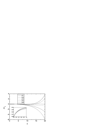
Figure 2: $\Delta\nu_{c}$ as a function of ${\cal I}$ calculated from (44) for different values of $z$ ($\eta=\eta_{c}$). The inset depicts the behavior of $\Delta\nu_{c}$ close to the origin.

Now we calculate $\tau^{2}$, $u$, $t_{0}$ and $t_{G}$ at $\eta=\eta_{c}$ using (32), (34), (38)-(39), (42) and formulas from Appendices B-D.

The dependence of $\tau^{2}$ on ${\cal I}$ at different values of the parameter $\lambda$ is plotted in Fig. 3. The explicit formula for $\tau_{SR}^{2}$ is given in Appendix C.

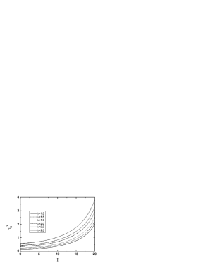
Figure 3: The dependence of $\tau^{2}$ on the ionicity for different $\lambda$ ($\eta=\eta_{c}$).

The coefficient $u$ and the shift in the mean-field critical temperature, $t_{0}$, as functions of ${\cal I}$ are plotted in Figs. 4 and 5. As is seen, quantities $\tau^{2}$, $t_{0}$ and $u$ are increasing functions of ${\cal I}$ in the whole region under consideration and their dependencies of ${\cal I}$ are at variance with those obtained in moreira-degama-fisher for the lattice model. Despite this fact, the behavior of the Ginzburg temperature as a function of ${\cal I}$ calculated in this work is qualitatively similar to that found in moreira-degama-fisher (see Figs. 6-8). Moreover, as in moreira-degama-fisher , the behavior of $t_{G}({\cal I})$ becomes nonmonotonic starting with some value of the attraction potential range ($\lambda$ in our case). One can see in Fig. 7 that, for $\lambda=2$, $t_{G}$ first drop off (at very small values of the ionicity) then increases slightly and at ${\cal I}\simeq 1.23$ again starts to decrease. In Fig. 8 the ratio of reduced Ginzburg temperatures, $t_{G}({\cal I})/t_{G}(0)$, is shown at different values of $\lambda$. It is worth noting that the non-monotonic behavior of $t_{G}({\cal I})$ becomes more pronounced as $\lambda$ increases.

Figure 4: The dependence of $u$ on the ionicity ${\cal I}$ ($\eta=\eta_{c}$).

Figure 5: The reduced shift of the mean-field critical temperature, $t_{0}$, as a function of ${\cal I}$ at $\eta=\eta_{c}$.

Figure 6: The reduced Ginzburg temperature, $t_{G}$, as a function of ${\cal I}$ at $\lambda=1.5$ ($\eta=\eta_{c}$). The inset depicts the behavior of $t_{G}({\cal I})$ close to the origin.

Figure 7: The same as in Fig. 6 but at $\lambda=2$.

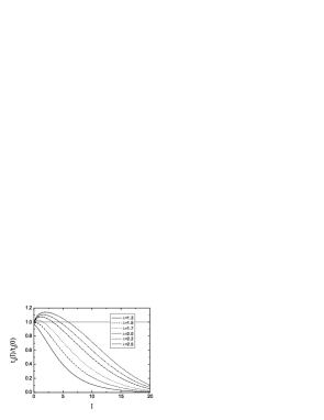
Figure 8: The ratio $t_{G}(I)/t_{G}(0)$ as a function of the ionicity at different values of $\lambda$ ($\eta=\eta_{c}$).

In Table 2 we compare our results for the ionicity dependence of the Ginzburg temperature (at $\lambda=1.5$) with the results obtained in moreira-degama-fisher for the lattice model as well as with experimental data for the crossover temperatures $t_{\times}$ (data for ${\cal I}$ and $t_{\times}$ are taken from moreira-degama-fisher ). The systems (b)-(d) correspond to the same ionic species ${\rm Bu_{4}NPic}$ within solvents of different dielectric constant. As is seen, in this case our results are in good agreement (qualitative and quantitative) with the experimental findings. The system (d) is ${\rm Na}$ in ${\rm NH_{3}}$ and, of course, might be described by the potential $\phi^{SR}(r)$ with the different attraction range $\lambda$. For instance, for $\lambda=2$ we obtain $t_{G}({\cal I}=6.97)=0.8\times 10^{-2}$ (see Fig. 7) that correlates with the experimental value $t_{\times}=0.6\times 10^{-2}$

Table 2: Experimentally assessed crossover temperature, $t_{\times}$, taken from moreira-degama-fisher : (a) tetra-$n$-butylammonium picrate (${\rm Bu_{4}NPic}$) in 1-tridecanol; (b) ${\rm Bu_{4}NPic}$ in 1-dodecanol; (c) ${\rm Bu_{4}NPic}$ in $75\%$ 1-dodecanol plus $25\%$ 1,4-butanediol; (d) ${\rm Na}$ in ${\rm NH_{3}}$; (e) tetra-$n$-pentylammonium bromide in water and the reduced Ginzburg temperature, $t_{G}$, found theoretically in moreira-degama-fisher and in this work.

System	Ionicity,${\cal I}$	$t_{\times}$	$t_{G}$ (moreira-degama-fisher )	$t_{G}$ (this work)
uncharged fluid	$0$	${\cal O}({\cal I})$	$1$	$\sim 0.09$
(a)	$17.9$	$\sim 10^{-3}$	$\sim 0.712$	$2.7\times 10^{-3}$
(b)	$16.8$	$\sim 0.9\times 10^{-2}$	$\sim 0.717$	$0.38\times 10^{-2}$
(c)	$8.9$	$\sim 3\times 10^{-2}$	$\sim 0.777$	$2.5\times 10^{-2}$
(d)	$6.97$	$\sim 0.6\times 10^{-2}$	$\sim 0.807$	$3.7\times 10^{-2}$
(e)	$\sim 1.4$	${\cal O}({\cal I})$	$1$	$\sim 0.09$

V Summary

In this paper we study the reduced Ginzburg temperature as a function of the interplay between the short- and long-range interactions. The ionic fluid is modelled as a charge asymmetric continuous system that includes additional short-range attractions. The model without Coulomb interactions exhibits a gas-liquid critical point belonging to the Ising class of criticality. We derive an effective GLW Hamiltonian for the model whose coefficients have the form of an expansion in powers of the ionicity. Using these coefficients we calculate a Ginzburg temperature depending on the ionicity. To this end we introduce a specific model which consists of charged hard spheres of the same diameter interacting through the additional square-well potentials. To study the effect of the interplay between short- and long-range interactions we change, besides the ionicity, the range of the square-well potential.

As a result, we obtain the similar tendency for the reduced Ginzburg temperature as in moreira-degama-fisher when the region of the short-range attraction increases i.e., its nonmonotonic character but with different numerical characteristics. However, our results demonstrate a much faster decrease of the Ginzburg temperature when the ionicity increases. We found a good qualitative and sufficient quantitative agreement with the experimental findings for ${\rm Bu_{4}NPic}$ in $n$-alkanols. This confirms the experimental observations that an interplay between the solvophobic and Coulomb interactions alters the temperature region of the crossover regime i.e., the increase of the ionicity that can be related to the decrease of dielectric constant leads to the decrease of the crossover region. We suggest that the quantitative discrepancy of the results for $t_{G}$ obtained in moreira-degama-fisher and in this work could be due to the fact, besides the difference in the symmetry of the two models, that the chemical potential (or density) dependence of the Hamiltonian coefficients was taken into account explicitly in our case.

It should be noted that in the approximation considered in this paper only the critical chemical potential depends explicitly on the charge magnitude. In order to obtain the charge dependence of the other quantities terms of order higher than $y^{2}$ should be taken into account into the effective Hamiltonian. Finally, we emphasize that the functional representation (7)-(8) allows to consider more complicated models in particular models including charge and size asymmetry.

VI Appendices

VI.1 Recurrence formulas for the cumulants Fourier space.

$${\mathfrak{M}}_{n}^{(0)}(k_{1},k_{2},\ldots,k_{n}) = {\widetilde{G}}_{n}(k_{1},k_{2},\ldots,k_{n})$$

$${\mathfrak{M}}_{n}^{(1)}(k_{1},k_{2},\ldots,k_{n}) = 0$$

$${\mathfrak{M}}_{n}^{(2)}(k_{1},k_{2},\ldots,k_{n}) = \left({\rm i}\right)^{2}\beta q_{\alpha}^{2}c_{\alpha}{\widetilde{G}}_{n-1}(k_{1},k_{2},\ldots,|{\mathbf{k}}_{n-1}+{\mathbf{k}}_{n}|)$$

$${\mathfrak{M}}_{n}^{(3)}(k_{1},k_{2},\ldots,k_{n}) = \left({\rm i}\right)^{3}\beta^{3/2}q_{\alpha}^{3}c_{\alpha}{\widetilde{G}}_{n-2}(k_{1},k_{2},\ldots,|{\mathbf{k}}_{n-2}+{\mathbf{k}}_{n-1}+{\mathbf{k}}_{n}|)$$

$${\mathfrak{M}}_{n}^{(4)}(k_{1},k_{2},\ldots,k_{n}) = \left({\rm i}\right)^{4}\beta^{2}\left\{3\left[q_{\alpha}^{2}c_{\alpha}\right]^{2}{\widetilde{G}}_{n-2}(k_{1},k_{2},\ldots,|{\mathbf{k}}_{n-2}+{\mathbf{k}}_{n-1}+{\mathbf{k}}_{n}|)\right.$$

$$\left.+\left(q_{\alpha}^{4}c_{\alpha}-3\left[q_{\alpha}^{2}c_{\alpha}\right]^{2}\right){\widetilde{G}}_{n-3}(k_{1},k_{2},\ldots,|{\mathbf{k}}_{n-3}+\ldots+{\mathbf{k}}_{n}|)\right\},$$

where ${\widetilde{G}}_{n}(k_{1},k_{2},\ldots,k_{n})$ is the Fourier transform of the $n$-particle truncated correlation function stell of a one-component hard sphere system and summation over repeated indices is meant.

VI.2 The nth-particle structure factors of a one component hard sphere systems in the Percus-Yevick approximation

$$S_{2}(0) = \frac{(1-\eta)^{4}}{(1+2\eta)^{2}},$$ (46)

$$S_{3}(0) = \frac{(1-\eta)^{7}(1-7\eta-6\eta^{2})}{(1+2\eta)^{5}},$$ (47)

$$S_{4}(0) = \frac{(1-\eta)^{10}(1-30\eta+81\eta^{2}+140\eta^{3}+60\eta^{4})}{(1+2\eta)^{8}},$$ (48)

$$S_{5}(0) = \frac{(1-\eta)^{13}(1-85\eta+957\eta^{2}-1063\eta^{3}-3590\eta^{4}-2940\eta^{5}-840\eta^{6})}{(1+2\eta)^{11}}$$ (49)

VI.3 Explicit expression for $\tau_{SR}^{2}$

Let us write the Ornstein-Zernike equation in the Fourier space

$$\tilde{S}_{2}(k)=\frac{1}{1-\rho\widetilde{c}(k)},$$ (50)

where $\widetilde{c}(k)$ is the Fourier transform of the Ornstein-Zernike direct correlation function hansen_mcdonald We have for $\widetilde{c}(k)$ in the Percus-Yevick approximation ashcroft-1

$$\rho\widetilde{c}(k) = -24\eta\left(\alpha k^{3}(\sin(k)-k\cos(k))+\beta k^{2}(2k\sin(k)-(k^{2}-2)\cos(k)-2)\right.$$ (51)

$$\left.+\frac{1}{2}\eta\alpha((4k^{3}-24k)\sin(k)-(k^{4}-12k^{2}+24)\cos(k)+24)\right)/k^{6},$$

where

$$\alpha=\frac{(1+2\eta)^{2}}{(1-\eta)^{4}},\qquad\beta=-6\frac{\eta(1+\frac{1}{2}\eta)^{2}}{(1-\eta)^{4}}$$

From (50) and (51) we get for $g^{2}$

$$g^{2}=\frac{\widetilde{G}_{22}(0)}{2\widetilde{G}_{2}(0)}=0.05\eta\frac{(4\eta^{6}-27\eta^{5}+84\eta^{4}-146\eta^{3}+144\eta^{2}-75\eta+16)}{(1+2\eta)^{2}(1-\eta)^{4}}.$$

Taking into account (38) we have $b_{SR}^{2}/\widetilde{w}_{S}(0)=0.1\lambda^{2}$. As a result, $\tau_{SR}^{2}$ is as follows

$$\tau_{SR}^{2}=-0.05\left(\eta\frac{(4\eta^{6}-27\eta^{5}+84\eta^{4}-146\eta^{3}+144\eta^{2}-75\eta+16)}{(1+2\eta)^{2}(1-\eta)^{4}}+2\lambda^{2}(1+t_{0}(y))\right),$$ (52)

where $t_{0}(y)$ is given by (42).

VI.4 Explicit expressions for the integrals used in equations (31)-(35)

Using $\sum_{\mathbf{k}}=\frac{V}{(2\pi)^{3}}\int\,({\rm d}{\mathbf{k}})$ we can present

$$\sum_{{\mathbf{k}}}\widetilde{\Delta}(k) = \frac{2}{\pi}\int_{0}^{\infty}{\rm d}x\,x^{2}{\overline{\Delta}}(x),$$ (53)

$$\sum_{{\mathbf{k}}}\left(\widetilde{\Delta}(k)\right)^{2} = \frac{48\eta}{\pi\langle N\rangle_{HS}}\int_{0}^{\infty}{\rm d}x\,x^{2}\left({\overline{\Delta}}(x)\right)^{2},$$ (54)

$$\sum_{{\mathbf{k}}}\widetilde{\Delta}(k)\widetilde{\Delta}^{(2)}(k) = \frac{32\eta\sigma^{2}}{\pi\langle N\rangle_{HS}}\int_{0}^{\infty}{\rm d}x\,x{\overline{\Delta}}(x)\left(2f_{1}(x)+xf_{2}(x)\right),$$ (55)

where the following notations are introduced:

$${\overline{\Delta}}(x) = \sin\left(x\right)\left({x}^{3}+{\kappa^{*}}^{2}\,\sin\left(x\right)\right)^{-1},$$ (56)

$$f_{1}(x) = \left({x}^{2}\left(\cos\left(x\right)x-3\,\sin\left(x\right)\right)\right)\left({x}^{6}+2\,{\kappa^{*}}^{2}{x}^{3}\,\sin\left(x\right)+{{\kappa^{*}}}^{4}-{{\kappa^{*}}}^{4}\cos^{2}\left(x\right)\right)^{-1}$$ (57)

$$f_{2}(x) = -x\left({x}^{5}\sin\left(x\right)+{x}^{2}{\kappa^{*}}^{2}+{\kappa^{*}}^{2}{x}^{2}\,\cos^{2}\left(x\right)+6\,\cos\left(x\right){x}^{4}-6\,{\kappa^{*}}^{2}x\,\sin\left(x\right)\cos\left(x\right)\right.$$ (58)

$$\left.-12\,{x}^{3}\sin\left(x\right)+6\,{\kappa^{*}}^{2}-6\,{\kappa^{*}}^{2}\,\cos^{2}\left(x\right)\right)\left({x}^{9}+3\,{\kappa^{*}}^{2}{x}^{6}\,\sin\left(x\right)+3\,{{\kappa^{*}}}^{4}{x}^{3}\right.$$

$$\left.-3\,{{\kappa^{*}}}^{4}{x}^{3}\cos^{2}\left(x\right)+{{\kappa^{*}}}^{6}\sin\left(x\right)-{{\kappa^{*}}}^{6}\sin\left(x\right)\cos^{2}\left(x\right)\right)^{-1}$$

with $x=k\sigma$ and ${\kappa^{*}}=\kappa_{D}\sigma=\sqrt{24y^{2}\eta}$ being the reduced Debye number.

References

- (1) R.R. Singh and K.S. Pitzer, J. Phys. Chem. 92, 6775 (1990).
- (2) J.M.H. Levelt Sengers and J. A. Given, Mol. Phys. 80, 899 (1993).
- (3) K.S. Pitzer, J. Phys. Chem. 99, 13070 (1995).
- (4) K. Gutkowski, M.A. Anisimov and J.V. Sengers, J. Chem. Phys. 114 3133 (2001).
- (5) W. Schröer and H. Weigärtner, Pure Appl. Chem. 76, 19 (2004).
- (6) W. Schröer, in Ionic Soft Matter: Modern Trends and Applications, edited by D. Henderson et al (Dordrecht: NATO ASI Series II, Springer, 2005), p. 143.
- (7) M.E. Fisher, J. Stat. Phys. 75, 1 (1994).
- (8) G. Stell, J. Stat. Phys. 78, 197 (1995).
- (9) F.H. Stillinger and R. Lovett, J. Chem. Phys. 48, 3858 (1968).
- (10) P.H. Vorontsov-Veliaminov, A.M. El’yashevich, L.A. Morgenshtern and V.P. Chasovshikh, Teplofiz. Vysokikh Temp.8, 277 (1970).
- (11) G. Stell, K.C. Wu and B. Larsen, Phys. Rev. Lett. 37, 1369 (1976).
- (12) Y. Zhou, S. Yeh and G. Stell, J. Chem. Phys.102,5785 (1995).
- (13) Y. Levin and M.E. Fisher, Physica A 225, 164 (1996).
- (14) M.E. Fisher and B.P. Lee, Phys. Rev. Lett. 77, 3361 (1996).
- (15) W. Schröer and V.C. Weiss, J. Chem. Phys. 109, 8504 (1998).
- (16) R.J.F. Leote de Carvalho and R. Evans, J. Phys.: Condensed Matter 7, 575 (1995).
- (17) J.-M. Caillol, D. Levesque and J.-J. Weis, J. Chem. Phys. 107, 1565 (1997).
- (18) J. Valleau and G. Torrie, J. Chem. Phys. 108, 5169 (1998).
- (19) P.J. Camp and G.N. Patey, J. Chem. Phys. 114, 399 (2001).
- (20) E. Luijten, M.E. Fisher and A.Z. Panagiotopoulos, J. Chem. Phys. 114, 5468 (2001).
- (21) J.-M. Caillol, D. Levesque and J.-J. Weis, J. Chem. Phys. 116, 10794 (2002).
- (22) O.V. Patsahan, Condens. Matter Phys.7, 35 (2004).
- (23) O.V. Patsahan, I. Mryglod and J.-M. Caillol, J. Phys.: Condens. Matter 17, L251 (2005).
- (24) E. Luijten, M.E. Fisher and A.Z. Panagiotopoulos, Phys. Rev. Lett. 88, 185701 (2002).
- (25) Y.C. Kim and M.E. Fisher, Phys. Rev. Lett. 92, 185703 (2004).
- (26) A. Ciach and G. Stell, J. Mol. Liq. 87, 253 (2000).
- (27) A. Ciach and G. Stell, Int. J. Mod. Phys. B 21, 3309 (2005).
- (28) A. Ciach, Phys. Rev. E 73, 066110 (2006).
- (29) O. Patsahan and I. Mryglod, J. Phys.: Condens. Matter 16, L235 (2004).
- (30) P.Chieux, M.J. Sienko, J. Chem. Phys. 53, 566 (1970).
- (31) T.Narayanan and K.S. Pitzer, J. Phys. Chem. 98, 9170 (1994).
- (32) T.Narayanan and K.S. Pitzer, J. Chem. Phys. 102, 8118 (1995).
- (33) M.A. Anisimov, J.Jacob, A. Kumar, V.A. Agayan and J.V. Sengers, Phys. Rev. Lett. 85, 2336 (2000).
- (34) K. Gutkowskii, M.A. Anisimov and J.V. Sengers, J. Chem. Phys. 114, 3133 (2001).
- (35) M. Kleemeier, S. Wiegand, W. Schröer and H. Weigärtner, J. Chem. Phys. 110, 3085 (1999).
- (36) A.G. Moreira, M.M. Telo de Gama and M.E. Fisher, J. Chem. Phys. 110, 10058 (1999).
- (37) D.A. McQuarrie, Statistical Mechanics (Harper-Collins, New York, 1976).
- (38) J.D. Weeks, D. Chandler and H.C. Andersen, J. Chem. Phys. 54, 5237 (1971).
- (39) G. Stell, in Phase Transitionss and Critical Phenomena, 5b, edited by C. Domb and M.S. Green (Academic Press, New York, 1975).
- (40) J.P. Hansen and I.R. McDonald, Theory of simple liquids (Academic Press, 1986).
- (41) N.W. Ashcroft and J. Lekner, Phys. Rev. B 83, 5237 (1966).