The Faiss Library
Abstract
Vector databases manage large collections of embedding vectors. As AI applications are growing rapidly, so are the number of embeddings that need to be stored and indexed. The Faiss library is dedicated to vector similarity search, a core functionality of vector databases. Faiss is a toolkit of indexing methods and related primitives used to search, cluster, compress and transform vectors. This paper first describes the tradeoff space of vector search, then the design principles of Faiss in terms of structure, approach to optimization and interfacing. We benchmark key features of the library and discuss a few selected applications to highlight its broad applicability.
1 Introduction
The emergence of deep learning has induced a shift in how complex data is stored and searched, noticeably by the development of embeddings. Embeddings are vector representations, typically produced by a neural network, whose main objective is to map (embed) the input media item into a vector space, where the locality encodes the semantics of the input. Embeddings are extracted from various forms of media: words [Mikolov et al., 2013, Bojanowski et al., 2017], text [Devlin et al., 2018, Izacard et al., 2021], images [Caron et al., 2021, Pizzi et al., 2022], users and items for recommendation [Paterek, 2007]. They can even encode object relations, for instance multi-modal text-image or text-audio relations [Duquenne et al., 2023, Radford et al., 2021].
Embeddings are employed as an intermediate representation for further processing, e.g. self-supervised image embeddings can input to shallow supervised image classifiers [Caron et al., 2018, Caron et al., 2021]. They are also leveraged as a pretext task for self-supervision, e.g. in SimCLR [Chen et al., 2020]. The purpose that we consider in this paper is when embeddings are used directly to compare media items. The embedding extractor is designed such that the distance between embeddings reflects the similarity between their corresponding media. As a result, neighborhood search in this vector space offers a direct implementation of similarity search between media items.
Embeddings are popular in industrial setting for tasks where end-to-end learning would not be cost-efficient. For example, a k nearest-neighbor classifier is more efficient to upgrade than a classification deep neural net. In that case, embeddings are particularly useful as a compact intermediate representation that can be re-used for several purposes. This explains why industrial database management systems (DBMS) that offer a vector storage and search functionality have gained adoption in the last years. These DBMS are at the junction of traditional databases and Approximate Nearest Neighbor Search (ANNS) algorithms. Until recently, the latter were mostly considered for specific use-cases or in research.
From a practical point of view, there are multiple advantages to maintain a clear separation of roles between the embedding extraction and the vector search algorithm. Both are bound by an “embedding contract” on the embedding distance:
-
•
The embedding extractor, which is typically a neural network in modern systems, is trained so that distances between embeddings are aligned with the task to perform.
-
•
The vector index aims at performing neighbor search among the embedding vectors as accurately as possible w.r.t. exact search results given the agreed distance metric.
Faiss is an industrial-grade library for ANNS. It is designed to be used both from simple scripts and as a building block of a DBMS. In contrast with other libraries that focus on a single indexing method, Faiss is a toolbox that contains indexing methods that commonly involve a chain of components (preprocessing, compression, non-exhaustive search, etc.). This is necessary: depending on the usage constraints, the most efficient indexing methods are different.
Let us also summarize what Faiss is not: Faiss does not extract features – it only indexes embeddings that have been extracted by a different mechanism; Faiss is not a service – it only provides functions that are run as part of the calling process on the local machine; Faiss is not a database – it does not provide concurrent write access, load balancing, sharding, consistency. The scope of the library is intentionally limited to focus on carefully implemented algorithms.
The basic structure of Faiss is the index. An index can store a number of database vectors that are progressively added to it. At search time, a query vector is submitted to the index. The index returns the database vector that is closest to the query vector in terms of Euclidean distance. There are many variants of this basic functionality: instead of just the nearest neighbor, nearest neighbors can be returned; instead of a fixed number of neighbors, only the vectors within a certain range can be returned; several vectors can be searched in parallel, in a batch mode; metrics other than the Euclidean distance are supported; the accuracy of search can be traded for speed or memory. The search can use either CPUs or GPUs.
The objective of this paper is to expose the design principles of Faiss. A similarity search library has to strike a tradeoff between different constraints (Section 3), which is addressed in Faiss with two main tools: vector compression (Section 4) and non-exhaustive search (Section 5). Faiss is engineered to be flexible and usable from other tools (Section 7). We also review a few applications of Faiss for trillion-scale indexing, text retrieval, data mining, and content moderation (Section 8). Throughout, we will refer with a specific style to functions or classes in the Faiss codebase111https://github.com/facebookresearch/faiss and documentation222https://faiss.ai/.
2 Related work
Indexing methods.
In the last decade, there has been a steady stream of papers about indexing methods that were published together with their reference implementations. In Faiss, we consider in particular algorithms that cover a wide spectrum of use-cases.
One of the most popular approach in industry is to employ Locality Sensitive Hashing as a way to compress embeddings into compact codes. In particular, the Cosine sketch [Charikar, 2002] produces binary vectors such that, in the corresponding Hamming space, the Hamming distance is an estimator of the cosine similarity between the original embeddings. The compactness of these sketches enables storing and therefore searching very large databases of media content [Lv et al., 2004], without the requirement to store the original embeddings. We refer the reader the early survey by [Wang et al., 2015] for research on binary codes.
Since the work by [Jégou et al., 2010], ANN based on quantization has emerged as a powerful alternative to binary codes [Wang et al., 2017]. We refer the reader to the survey by [Matsui et al., 2018] that discusses numerous research works related to quantization-based compact codes.
LSH is also often referring to indexing with multiple partitions, such as E2LSH [Datar et al., 2004]. We do no consider them because they are not performing as well as learned partitions on real data [Paulevé et al., 2010]. Early data-aware methods that proved successful on large datasets include multiple partitions based on kd-tree or hierarchical k-means in [Muja and Lowe, 2014]. They are often combined with compressed-domain representation and are especially appropriate for very large-scale settings [Jegou et al., 2008, Jégou et al., 2010].
After the introduction of the NN-descent algorithm [Dong et al., 2011], ANN algorithms based on graphs have emerged as a viable alternative to methods based on space partitioning. In particular HNSW, which is the most popular current indexing method [Malkov and Yashunin, 2018] for medium-sized dataset is implemented in HNSWlib.
Software packages.
Most of the research works on vector search were open-sourced, and some of these evolved in relatively comprehensive software packages for vector search. FLANN includes several index types and a distributed implementation described extensively in the paper [Muja and Lowe, 2014]. The first implementation of product quantization relied on the Yael library [Douze and Jégou, 2014], that already had a few of the Faiss principles: optimized primitives for clustering methods (GMM and k-means), scripting language interface (Matlab and Python) and benchmarking operators. The NMSlib package, intended for text retrieval was the first package to include HNSW [Boytsov et al., 2016] and also offers several index types. The HNSWlib library later became the reference implementation of HNSW [Malkov and Yashunin, 2018]. Google’s SCANN library is mainly a thoroughly optimized implementation of IVFPQ [Jégou et al., 2010] on SIMD and includes several index variants for various database scales. SCANN was open-sourced together with the paper [Guo et al., 2020], which does not describe what makes the library so fast: its engineering optimization. Diskann [Subramanya et al., 2019] is Microsoft’s foundational graph-based vector search library, initially built to exploit hybrid RAM/flash memory, but that also offers a RAM-only version called Vamana. It was later extended to perform efficient updates [Singh et al., 2021], out-of-distribution searches [Jaiswal et al., 2022] and filtered searches [Gollapudi et al., 2023].
Faiss was open-sourced simultaneously with the release of the paper [Johnson et al., 2019] that describes the GPU implementation of several index types. The present paper complements this previous work by describing the library as a whole.
In parallel, numerous software libraries from the database world were extended or developed to do vector search. Milvus [Wang et al., 2021] uses its Knowhere library, which relies on Faiss as one of its core engines. Pinecone [Bruch et al., 2023] initially relied on Faiss. The engine has since been rewritten. Weaviate [van Luijt and Verhagen, 2020] is a composite retrieval engine that includes vector search.
Benchmarks and competitions.
The leading benchmark for million-scale datasets is ANN-benchmarks [Aumüller et al., 2020] that now compares about 50 implementations of ANNS. This benchmark was upgraded with the big-ANN [Simhadri et al., 2022a] challenge, that includes 6 datasets with 1 billion vectors each. Faiss was used as a baseline for the challenge and multiple submissions derived from Faiss. The 2023’s edition of the challenge is at a more modest scale (10M vectors) but the tasks are more elaborate. For instance there is a filtered track for which Faiss was a baseline method.
Datasets
The datasets used to evaluate vector search are typical for the tasks that vector search performs. Early datasets are based on keypoint features like SIFT [Lowe, 2004] used in image matching. We use BIGANN [Jégou et al., 2011b], a dataset of 128-dimensional SIFT features. Later, when global image descriptors produced by neural nets became popular, the Deep1B dataset was released [Babenko and Lempitsky, 2016], with 96-dimensional image features extracted with Google LeNet [Szegedy et al., 2015]. For this paper we introduce a dataset of 768-dimensional Contriever text embeddings [Izacard et al., 2021] that are compared with inner product similarity. The embeddings are computed on English Wikipedia passages. The higher dimension of these embeddings is typical for contemporary applications.
Each dataset has 10k query vectors, 20M to 350M training vectors. We indicate the size of the database explicitly, for example “Deep1M” means the database contains the 1M first vectors of deep1B. The training, database and query vectors are sampled randomly from the same distribution, we don’t address out-of-distribution data in this paper [Jaiswal et al., 2022, Baranchuk et al., 2023].
3 Performance axes of a vector search library
Vector search is a well-defined, unambiguous operation. In its simplest formulation, given a set of database vectors and a query vector , it computes
| (1) |
This can be computed with a direct algorithm by iterating over all database vectors: this is brute force search. A slightly more general and complex operation is to compute the nearest neighbors of :
| (2) |
This is what the search method of a Faiss index returns. A related operation is to find all the elements that are within some distance to the query:
| (3) |
which is computed with the range_search method.
Distance measures.
In the equations above, we leave the definition of the distance undefined. The most commonly used distances in Faiss are the L2 distance, the cosine similarity and the inner product similarity (for the latter two the should be replaced with an ). These simple measures have useful analytical properties: for example, they are invariant under -dimensional rotations.
There are many relationships between the measures. They can be made equivalent by preprocessing transformations on the query and/or the database vectors. Table 1 summarizes the preprocessing transformations that are applicable for various bridges. Some were already identified [Bachrach et al., 2014, Hong et al., 2019], others are new.
Note that vectors transformed in this way have a very anisotropic distribution [Morozov and Babenko, 2018] and can be “harder” to index. In particular, for product or scalar quantization, the additional dimension incurred for many transformations is not homogeneous with other dimensions. See Section 4.2 for mitigations.
| index metric | L2 | IP | cos |
| wanted metric | |||
| L2 | identity | ||
| IP | identity | ||
| cos | identity |
3.1 Brute force search
Implementing brute force search efficiently is not trivial [Chern et al., 2022, Johnson et al., 2019]. It requires (1) an efficient way of computing the distances and (2) for k-nearest neighbor search, an efficient way of keeping track of the smallest distances.
Computing distances in Faiss is performed either by direct distances computations, or, when query vectors are provided in large enough batches, using a matrix multiplication decomposition [Johnson et al., 2019, equation 2]. The Faiss functions are exposed in knn and knn_gpu for CPU and GPU respectively.
Collecting the top- smallest distances is usually done via a binary heap on CPU [Douze and Jégou, 2014, section 2.1] or a sorting network on GPU [Johnson et al., 2019, Ootomo et al., 2023]. For larger values of , it is more efficient to use a reservoir: an unordered result buffer of size that is resized to when it overflows.
Brute-force search gives accurate results. However, for large, high-dimensional datasets this approach becomes slow. In low dimensions, there are branch-and-bound methods that yield exact search results. However, in large dimensions they provide no speedup over brute force search [Weber et al., 1998].
In these cases, we have to resort to approximate nearest neighbor search (ANNS).
3.2 Metrics for Approximate Nearest Neighbor Search
With ANNS, the user accepts imperfect results, which opens the door to a new solution design space. The database may be preprocessed into an indexing structure, rather than just being stored as a plain matrix.
Accuracy metrics.
In ANNS the accuracy is measured as a difference with the exact search results. Note that this is an intermediate goal: the end-to-end accuracy depends on (1) how well the distance metric correlates with the item matching objective and (2) the quality of ANNS, which is what we measure here.
This accuracy metric is compared to the ground-truth results from Equation (1).
The accuracy for k-nearest neighbor search is generally evaluated as the “-recall@”, which is the fraction of the ground-truth nearest neighbors that are in the first search results. Most often or (in which case the measure is a.k.a. “intersection measure”). When = = , the recall measure and intersection are the same, and the recall is called “accuracy”. Note, in some publications [Jégou et al., 2010], recall@ means 1-recall@, while in others [Simhadri et al., 2022b] it corresponds to -recall@.
For range search, there are two thresholds: the ground-truth threshold of Equation 3 and a second threshold applied at search time. By sweeping from small to large, the result list increases. Comparing the search-time with the ground-truth yield a precision and recall, so the sweep produces a precision-recall curve. The area under the PR-curve is the mean average precision score of range search.
For vector codecs, the metric of choice is the mean squared error (MSE) between the original vector and the reconstructed vector. For an encoder and a decoder , the MSE is:
| (4) |
Resource metrics.
The other axes of the tradeoff are related to computing resources. During search, the search time and memory usage are the main constraints, the experiments in this paper operate mainly with these. The memory usage can be smaller than that of the original vectors, if compression is used.
The index may need to store training data, which incurs a constant memory overhead before any vector is added to the index. The index can also add per-vector memory overhead to the memory used to store each vector. This is the case for graph indexes, that need to store a graph for each node.
The index building time is also a resource constraint. It may be decomposed into a training time, a fixed cost that needs to be paid regardless of the number of vectors added to the index and the addition time per vector.
The memory usage is more complex to grasp for settings with hybrid storage, for example RAM + flash + disk or GPU memory + RAM. In that case, there is usually a small amount of fast memory and a larger amount of slower memory, so several access speeds need to be taken into account.
In distributed settings or flash-backed storage, the relevant metric is the number of I/O operations (IOPS). Every read operation fetches a whole page (of e.g. 4 kiB). Therefore, random accesses to scalar elements are particularly inefficient. It is better to organize the data layout to minimize the IOPs [Subramanya et al., 2019]. Another low-level metric is the amount of extra memory needed to pre-compute lookup tables used to speed up search, which can be a limiting factor.
3.3 Tradeoffs
Most often only a subset of metrics matter. For example, when a very large number of searches are performed on a fixed index, index building time does not matter. Or when the number of vectors is so small that the raw database fits in RAM multiple times, then memory usage does not matter. We call the metrics that we care about the active constraints. Note that accuracy is always an active constraint because it can be traded off against every single other constraint. In extreme cases where accuracy does not matter, an index that returns random results would be sufficient (and Faiss does actually provide an IndexRandom used in some benchmarking tasks).
In the following sections, we will most often consider that the active constraints are speed, memory usage and accuracy. This can be done, for example, by fixing a memory budget and measuring the speed and accuracy of several index types and hyperparameter settings.
3.4 Exploring search-time settings
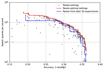
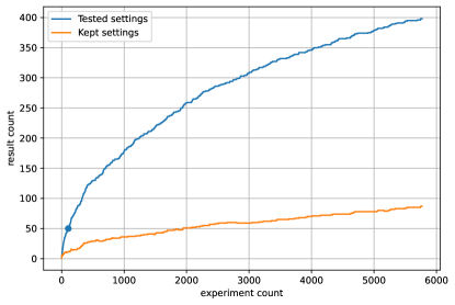
For a fixed index, there are often one or several search-time hyper-parameters that shift the tradeoff between speed and accuracy. This is for example the nprobe hyperparameter for an IndexIVF, see Section 5. In general, we define hyperparameters as scalar values such that when the value is higher, the speed decreases and the accuracy increases. We can then keep only the Pareto-optimal settings, defined as settings that are the fastest for a given accuracy, or equivalently that have the highest accuracy for a given time budget [Sun et al., 2023a].
Exploring the Pareto-optimal frontier when there is a single hyper-parameter consists in sweeping over its values and measuring the corresponding speed and accuracy. This exploration can be done with a certain level of granularity.
When there are several hyperparameters, the Pareto frontier can be recovered by exhaustively testing the Cartesian product of these parameters. However, the number of settings to test grows exponentially with the number of parameters.
Pruning the parameter space.
There is an interesting optimization in this case, which enables efficient pruning. We note a tuple of hyper-parameters , and a partial ordering on : . Let and be the speed and accuracy obtained with this tuple of parameters. is the set of Pareto-optimal settings:
| (5) |
Since the individual parameters have a predictable, monotonic effect on speed and accuracy, we have the following implication:
| (6) |
Thus, if a subset of settings is already evaluated, the following upper bounds hold for a new setting :
| (7) | |||||
| (8) |
If any previous evaluation Pareto-dominates these bounds, the setting does not need to be evaluated:
| (9) |
In practice, we evaluate settings from in a random order. The pruning becomes more and more effective throughout the process. It is also more effective when the number of parameters is larger. Figure 1 shows an example with combined parameter settings. The pruning from Eq. 9 reduces this to 398 experiments, out of which are optimal. The Faiss object OperatingPoints implements this logic.
3.5 Exploring the index space
| No encoding | PQ encoding | scalar quantizer | |
|---|---|---|---|
| Flat | IndexFlat | IndexPQ | IndexScalarQuantizer |
| IVF | IndexIVFFlat | IndexIVFPQ | IndexIVFScalarQuantizer |
| HNSW | IndexHSNWFlat | IndexHNSWPQ | IndexHNSWScalarQuantizer |
Faiss includes a benchmarking framework that explores the index design space to find the parameters that optimally trade off accuracy, memory usage and search time. The benchmark generates candidate index configurations to evaluate, sweeps both construction-time and search-time parameters, and measures these metrics. The accuracy metric is selected as applicable, n-recall@m for k-nearest neighbors, mean average precision for range search, and mean squared error for vector codecs, and it can be further customized.
Decoupling encoding and non-exhaustive search options.
Beyond a certain scale, search time is determined by the number of distance computations between the query vector and database vectors. The non-exhaustive search methods in Faiss are either based on a clustering, or on a graph exploration, see Section 5. Another limiting factor of vector search is the memory usage per vector (RAM or disk). In order to fit more vectors, they need to be compressed. Faiss implements a range of compression options, see Section 4.
Therefore, Faiss indexes are built as a combination of pruning method and a compression method, see Table 2. In the following sections, we explore the options in these two directions.
To evaluate a large number of index configurations efficiently, the benchmarking framework takes advantage of this compositional nature of Faiss indices during the index training and search. The training of vector transformations and k-means clustering for IVF coarse quantizers are factored out and reused during the training of compatible indices. Coarse quantizers and IVF indices are first trained and evaluated separately, the parameter space is pruned as described in the previous section, and only the combinations of Pareto-optimal components are benchmarked together. It is implemented in bench_fw.
3.6 Refining (IndexRefine)
It is possible to combine a fast and inaccurate indexing method with a slower and more accurate search [Jégou et al., 2011b, Subramanya et al., 2019, Guo et al., 2020]. This is done by querying the fast index to retrieve a shortlist of results. The more accurate search then computes more accurate search results only for the shortlist. This requires the accurate index to store the vectors in a way that allows efficient random access to possibly-compressed database vectors. Some implementations use a slower storage (e.g. flash) for the second index [Subramanya et al., 2019, Sun et al., 2023b].
For the first-level index, the relevant accuracy metric is the recall at the rank that will be used for re-ranking. The recall @ rank 1000 can thus sometimes be a relevant metric, even if the end application does not use the 1000th neighbor at all.
Several methods are also based on this refining principle but do not use two separate indexes. Instead, they use two ways of interpreting the same compressed vectors: a fast and inaccurate decoding and a slower but more accurate decoding [Douze et al., 2016, Douze et al., 2018, Morozov and Babenko, 2019, Amara et al., 2022] are based on this principle. The polysemous codes method [Douze et al., 2016] is implemented in Faiss’s IndexIVFPQ.
4 Compression levels
Faiss supports various vector codecs: these are methods to compress vectors so that they take up less memory. A compression method , a.k.a. a quantizer, converts a continuous multi-dimensional vector to an integer or equivalently a fixed size bit string. The length of the corresponding bit string is called the code size. The decoder reconstructs an approximation of the vector from the integer. Since the number of distinct integers of a certain size is finite, the decoder can only reconstruct a finite number of distinct vectors.
The search of Equation (1) becomes approximate:
| (10) |
Where the codes are precomputed and stored in the index. This is the asymmetric distance computation (ADC) [Jégou et al., 2010]. The symmetric distance computation (SDC) corresponds to the case when the query vector is also compressed:
| (11) |
Most Faiss indexes perform ADC as it is more accurate: there is no accuracy loss on the query vectors. SDC is useful when there is also a storage constraint on the queries or for indexing methods for which SDC is faster to compute than ADC.
4.1 The vector codecs
The k-means vector quantizer (Kmeans)
The ideal vector quantizer minimizes the MSE between the original and the decompressed vectors. This is formalized in the Lloyd necessary conditions for the optimality of a quantizer [Lloyd, 1982].
The k-means clustering algorithm can be seen as a quantizer that directly applies the Lloyd optimality conditions [Amara et al., 2022]. The centroids of k-means are an explicit enumeration of all possible vectors that can be reconstructed. Thus the size of the bit strings that the k-means quantizer produces is bits.
The k-means vector quantizer is very accurate but the memory usage and encoding complexity grow exponentially with the code size. Therefore, k-means is impractical to use beyond 3-byte codes, corresponding to 16M centroids.
Scalar quantizers
Scalar quantizers encode each dimension of a vector independently.
A very classical and simple scalar quantizer is LSH (IndexLSH), where each vector component is encoded in a single bit by comparing it to a threshold. The threshold can be set to 0 or trained. Faiss further supports efficient search of binary vectors via the IndexBinary objects, see Section 4.5.
The Faiss ScalarQuantizer also supports uniform quantizers that encode a vector component into 8, 6 or 4 bits – referred to as SQ8, SQ6, SQ4.
A per-component scale and offset determine which values are reconstructed.
They can be set separately for each dimension or uniformly on the whole vector.
The IndexRowwiseMinMax stores vectors with per-vector normalizing coefficients.
The ranges are trained beforehand on a set of representative vectors.
The lower-precision float16 representation is also considered as a scalar quantizer, SQfp16.
Multi-codebook quantizers.
Faiss contains several multi-codebook quantization options. They are built from vector quantizers that can reconstruct distinct values each. The codes produced by these methods are of the form , i.e. each code indexes one of the quantizers. The number of reconstructed vectors is and the code size is thus .
The product quantizer (ProductQuantizer, also noted PQ) is a simple multi-codebook quantizer that splits the input vector into sub-vectors and quantizes them separately [Jégou et al., 2010] with a k-means quantizer.
At reconstruction time, the individual reconstructions are concatenated to produce the final code.
In the following, we will use the notation PQ6x10 for a product quantizer with 6 sub-vectors each encoded in 10 bits (, ).
Additive quantizers are a family of multi-codebook quantizers where the reconstructions from sub-quantizers are summed up together. Finding the optimal encoding for a vector given the codebooks is NP-hard, so practical additive quantizers are heuristics to find near-optimal codes.
Faiss supports two types of additive quantizers.
The residual quantizer (ResidualQuantizer) proceeds sequentially, by encoding the difference (residual) of the vector to encode and the one that is reconstructed by the previous sub-quantizers [Chen et al., 2010].
The local search quantizer (LocalSearchQuantizer) starts from a sub-optimal encoding of the vector and locally explores neighbording codes in a simulated annealing process [Martinez et al., 2016, Martinez et al., 2018].
We use notations LSQ6x10 and RQ6x10 to refer to additive quantizers with 6 codebooks of size .
Faiss also supports a combination of PQ and residual quantizer, ProductResidualQuantizer. In that case, the vector is split in sub-vectors that are encoded independently with additive quantizers [Babenko and Lempitsky, 2015].
The codes from the sub-quantizers are concatenated.
We use the notation PRQ2x6x10 to indicate that vectors are split in 2 and encoded independently with RQ6x10, yielding a total of 12 codebooks of size .
Hierarchy of quantizers
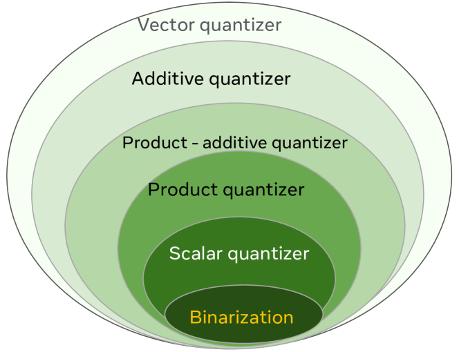
Although this is not by design, it turns out that there is a strict ordering between the quantizers described before. This means that quantizer can have the same set of reproduction values as quantizer : it is more flexible and more data adaptive. The hierarchy of quantizers is shown in Figure 2:
-
1.
the binary representation with bits +1 and -1 can be represented as a scalar quantizer with 1 bit per component;
-
2.
the scalar quantizer can be represented as a product quantizer with 1 dimension per sub-vector and uniform per-dimension quantizer;
-
3.
the product quantizer can be represented as a product-additive quantizer where the additive quantizer has a single level;
-
4.
the product additive quantizer is an additive quantizer where within each codebook all components outside one sub-vector are set to 0 [Babenko and Lempitsky, 2014];
-
5.
the additive quantizer (and any other quantizer) can be represented as a vector quantizer where the codebook entries are the explicit enumeration of all possible reconstructions.
The implications of this hierarchy are (1) the degrees of freedom for the reproduction values of quantizer are larger than for , so it is more accurate (2) quantizer has a higher capacity so it consumes more resources in terms of training time and storage overhead than . In practice, the product quantizer often offers a good tradeoff, which explains its adoption.
4.2 Vector preprocessing
To take advantage of some quantizers, it is beneficial to apply transformations to the input vectors prior to encoding them. Many of these transformations are -dimensional rotations, that do not change comparison metrics like cosine, L2 and inner product.
Scalar quantizers assign the same number of bits per vector component. However, for distance comparisons, if specific vector components have a higher variance, they have more impact on the distances. In other works, a variable number of bits are assigned per component [Sandhawalia and Jégou, 2010]. However, it is simpler to apply a random rotation to the input vectors, which in Faiss can be done with a RandomRotationMatrix. The random rotation spreads the variance over all the dimensions without changing the measured distances.
An important transform is the Principal Component Analysis (PCA), that reduces the number of dimensions of the input vectors to a user-specified . This operation (PCAMatrix) is the orthogonal linear mapping that best preserves the variance of the input distribution. It is often beneficial to apply a PCA to large input vectors before quantizing them as k-means quantizers are more likely to “fall” in local minima in high-dimensional spaces [Liu et al., 2015, Jégou et al., 2011a].
The OPQ transformation [Ge et al., 2013] is a rotation of the input space that decorrelates the distribution of each sub-vector of a product quantizer333In Faiss terms, OPQ and ITQ are preprocessing transformations. The actual quantization is performed by a subsequent product quantizer or binarization step.. This makes PQ more accurate in the case where the variance of the data is concentrated on a few components. The Faiss implementation OPQMatrix combines OPQ with a dimensionality reduction.
The ITQ transformation [Gong et al., 2012] similarly rotates the input space prior to binarization (ITQMatrix).
4.3 Faiss additive quantization options
We look in more detail into the additive quantizer variants: the residual quantizer and local search quantizer. They are more complex than most quantizers because the index building time has to be considered, since the accuracy of a fixed-size encoding can always be increased at the cost of an increased encoding time.
Additive quantizers rely on codebooks of size in dimension . The decoding of code is
| (12) |
Thus, decoding is unambiguous. However, there is no practical way to do exact encoding, let alone training the codebooks. Enumerating all possible encodings is of exponential complexity in .
| Deep1M | Contriever1M |
|---|---|
 |
 |
The residual quantizer (RQ).
RQ encoding is sequential. At stage of the encoding of , RQ picks the entry that best reconstructs the residual of w.r.t. the previous encoding steps:
| (13) |
This greedy approach tends to get trapped in local minima. As a mitigation, the encoder maintains a beam of max_beam_size of possible codes and picks the best code at stage . This parameter adjusts the tradeoff between encoding time and accuracy.
To speed up the encoding, the norm of Equation (13) can optionally be decomposed into the sum of:
-
•
is precomputed and stored;
-
•
is the encoding error of the previous step ;
-
•
is computed on entry to the encoding (it is the only component whose computation complexity depends on );
-
•
is also precomputed.
This decomposition is used when use_beam_LUT is set. It is interesting only if is large and when is small because the storage and compute requirements of the last term grow quadratically with .
The local search quantizer (LSQ).
At encoding time, LSQ starts from a suboptimal encoding of the vector and proceeds with a simulated annealing optimization to refine the codes. In each iteration of the optimization step, LSQ adds perturbations to the codes and then uses Iterated Conditional Mode (ICM) to optimize the new encoding. The number of optimization steps is set with encode_ils_iters. The LSQ codebooks are trained via an expectation-maximization procedure (similar to k-means).
Compressed-domain search
consists in computing distances without decompressing the stored vectors. It is acceptable to perform pre-computations on the query vector because it is assumed that the cost of these pre-computations will be amortized over many query-to-code distance comparisons.
Additive quantizer inner products can be computed in the compressed domain:
| (14) |
The lookup tables are computed when a query vector comes in, similar to product quantizer search [Jégou et al., 2010].
In contrast with the product quantizer, this decomposition does not work to compute L2 distances when the codebooks are not orthgonal. As a workaround, Faiss uses the decomposition [Babenko and Lempitsky, 2014]
| (15) |
Thus, the term must be available at search time. Depending on the setting of AdditiveQuantizer.search_type it can be appended in the stored code (ST_norm_float32), possibly compressed (ST_norm_qint8, ST_norm_qint4,…). It cal also be computed on-the-fly (ST_norm_from_LUT) with
| (16) |
Where the norms and dot products are stored in the same lookup tables as the one used for beam search. Therefore, it is a tradeoff between memory overhead to store codes and search time overhead.
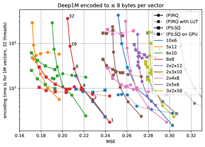
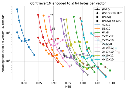
Figure 3 shows the tradeoff between encoding time and MSE. For a given code size, it is more accurate to use a smaller number of sub-quantizers and a higher . GPU encoding for LSQ does not help systematically. The LUT-based encoding of RQ is interesing for RQ/PRQ quantization when the beam size is larger. For the 64-byte regime, we observe that LSQ is not competitive with RQ. PLSQ and PRQ progressively become more competitive for larger memory budgets. They are also faster, since they operate on smaller vectors.
4.4 Vector compression benchmark
Figure 4 shows the tradeoff between code size and accuracy for many variants of the codecs. Additive quantizers are the best options for small code sizes. For larger code sizes it is beneficial to independently encode several sub-vectors with product-additive quantizers. LSQ is more accurate than RQ for small codes, but does not scale well to longer codes. Note that product quantizers are a bits less accurate than the additive quantizers but given how efficient they are this remains an attractive option. The scalar quantizers perform well for very long codes and are even faster. The 2-level PQ options are what an IVFPQ index uses as encoding: a first-level coarse quantizer and a second level refinement of the residual (more about this in Section 5.1).
4.5 Binary indexes
Binary quantization with symmetric distance computations is a pattern that has been commonly used [Wang et al., 2015, Cao et al., 2017]. In this setup, distances are computed in the compressed domain as Hamming distances. Equation (11) reduces to:
| (17) |
where . Although binary quantizers are crude approximations for continuous domain distances, the Hamming distances are integers in , that are fast to compute, do not require any specific context, and are easy to calibrate in practice.
The Faiss IndexBinary indexes support addition and search directly from binary vectors. They offer a compact representation and leverage optimized instructions for distance computations.
The simplest IndexBinaryFlat index performs exhaustive search. Three options are offered for non-exhaustive search:
-
•
IndexBinaryIVF is a binary counterpart for the inverted-list IndexIVF index described in 5.1.
-
•
IndexBinaryHNSW is a binary counterpart for the hierarchical graph-based IndexHNSW index described in 5.2.
-
•
IndexBinaryHash uses prefix vectors as hashes to cluster the database (rather than spheroids as with inverted lists), and searches only the clusters with closests prefixes.
Finally, a convenience IndexBinaryFromFloat index is provided that simply wraps an arbitrary index and offers a binary vector interface for its operations.
5 Non-exhaustive search
Non-exhaustive search is the cornerstone of fast search implementations for medium-sized datasets. In that case, the aim of the indexing method is to quickly focus on a subset of database vectors that are most likely to contain the search results.
An early method to do this is Locality Sensitive Hashing (LSH). It amounts to projecting the vectors on a random direction [Datar et al., 2004]. The offsets on that direction are then discretized into buckets where the database vectors are stored. At search time, the buckets nearest to the query vector’s projection are visited. In practice, several projection directions are needed to make it accurate, at the cost of search time. A fundamental drawback of this method is that it is not data-adaptive, although some improvements are possible [Paulevé et al., 2010].
An alternative way of pruning the search space is to use tree-based indexing. In that case, the dataset is stored in the leaves of a tree [Muja and Lowe, 2014]. When querying a vector, the search starts at the root node. At each internal node, the search descends into one of the child nodes depending on a decision rule. The decision rule depends on how the tree was built: for a KD-tree it is the position w.r.t. a hyperplane, for a hierarchical k-means, it is the proximity to a centroid.
Both in the case of LSH and tree-based methods, the hope is to extend classical database search structures to vector search, because they have a favorable complexity (constant or logarithmic in ). However, it turns out that these methods do not scale well for dimensions above 10.
Faiss implements two non-exhaustive search approaches that operate at different memory vs. speed tradeoffs: inverted file and graph-based.
5.1 Inverted files
IVF indexing is a technique that clusters the database vectors at indexing time. This clustering uses a vector quantizer (the coarse quantizer) that outputs distinct indices (Faiss’s nlist parameter). The coarse quantizer’s reproduction values are called centroids. The vectors of each cluster (possibly compressed) are stored contiguously into inverted lists, forming an inverted file (IVF). At search time, only a subset of clusters are visited (a.k.a. nprobe). The subset is formed by searching the nearest centroids, as in Equation (2).
Setting the number of lists.
The parameter is central. In the simplest case, when is fixed, the coarse quantizer is exhaustive, the inverted lists contain uncompressed vectors, and the inverted lists are all the same size, then the number of distance computations is
| (18) |
which reaches a minimum when . This yields the usual recommendation to set proportional to .
In practice, this is just a rough approximation because (1) the has to increase with the number of lists in order to keep a fixed accuracy (2) often the coarse quantizer is not exhaustive itself, so the quantization uses fewer than distance computations, for example it is common to use a non-exhaustive HNSW index to perform the coarse quantization.
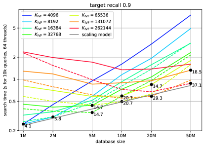
Figure 5 shows the optimal settings of for various database sizes. For a small , the coarse quantization runtime is negligible and the search time increases linearly with the database size. For larger datasets it is beneficial to increase the . As in equation (18), the ratio is roughly 15 to 20. Note that this ratio depends on the data distribution and the target accuracy. Interestingly, in a regime where is larger than the optimal setting for (e.g. and 5M), the needed to reach the target accuracy decreases with the dataset size, and so does the search time. This is because when is fixed and increases, for a given query vector, the nearest database vector is either the same or a new one that is closer, so it is more likely to be found in a quantization cluster nearer to the query.
With a faster non-exhaustive coarse quantizer (e.g. HNSW) it is even more useful to increase for larger databases, as the coarse quantization becomes relatively cheap. At the limit, when , then all the work is done by the coarse quantizer. However, in that case the limiting factor becomes the memory overhead of the coarse quantizer.
By fitting a model of the form to the timings of the fastest index in Figure 5, we can derive a scaling rule for the IVF indexes:
| target recall@1 | 0.5 | 0.75 | 0.9 | 0.99 |
|---|---|---|---|---|
| power | 0.29 | 0.30 | 0.34 | 0.45 |
Thus, with this model, the search time increases faster for higher accuracy targets, but , so the runtime dependence on the database size is below .
Encoding residuals.
In general, it is more accurate to compress the residuals of the database vectors w.r.t. the centroids [Jégou et al., 2010, Equation (28)]. This is because the norm of the residuals is lower than that of the original vectors, or because residual encoding is a way to take into account a-priori information from the coarse quantizer. In Faiss, this is controlled via the IndexIVF.by_residual flag, which is set to true by default.
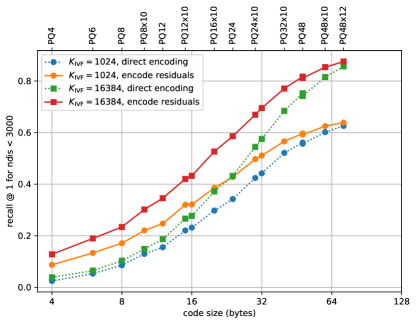
Figure 6 shows that encoding residuals is beneficial for shorter codes. For larger codes, the contribution of the residual is less important. Indeed, as the original data is 96-dimensional, it can be compressed to 64 bytes relatively accurately. Note that using higher also improves the accuracy of the quantizer with residual encoding. From a pure encoding point of view, the additional bits of information brought by the coarse quantizer ( or ) improve the accuracy more when used in this residual encoding than if they would added to increase the size of a PQ.
Spherical clustering for inner product search
Efficient indexing for maximum inner product search (MIPS) faces multiple issues: the distribution of query vectors is often different from the database vector distribution, most notably in recommendation systems [Paterek, 2007]; the MIPS datasets are diverse, an algorithm that obtains a good performance on some dataset will perform badly on another. Besides, [Morozov and Babenko, 2018] show that using the preprocessing formulas in Section 3 is a suboptimal way of indexing for MIPS.
Several specialized clustering and indexing methods were developed for MIPS [Guo et al., 2020, Morozov and Babenko, 2018]. Instead, Faiss implements a simple modification of k-means clustering, spherical k-means [Dhillon and Modha, 2001], that normalizes the k-means centroids at each iteration.
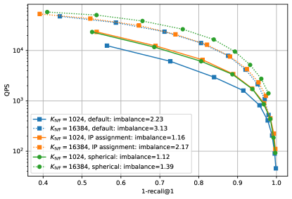
The MIPS issues appear strongly when vectors are of very different norms (when the database vectors are normalized, MIPS becomes equivalent to L2 search). For IVF, this manifests itself with a high imbalance factor, which is the relative variance of inverted list sizes [Tavenard et al., 2011]. At search time, if the inverted lists are perfectly balanced (i.e. all have the same length), this factor is 1. If they are unbalanced, the number of distances computed for a given increases with the imbalance factor.
The imbalance is mainly due to high-norm centroids that attract the database vectors in their clusters. To avoid this, we can normalize the centroids at each iteration.
Figure 7 shows that for the contriever MIPS dataset, the imbalance factor is quite high. It can be reduced by using IP assignment instead of L2, and even more by L2-normalizing the centroids at each k-means iteration (spherical is set to true).
Big batch search
A common use case for ANNS is search with very large query batches. This appears for applications such as large-scale data deduplication. In this case, rather than loading an entire index in memory and processing queries one small batch at a time, it can be more memory-efficient to load only the quantizer, quantize the queries, and then iterate over the index by loading it one chunk at a time. Big-batch search is implemented in the module contrib.big_batch_search.
5.2 Graph based
Graph-based indexing consists in building a directed graph whose nodes are the vectors to index. At search time, the graph is explored by following the edges towards the nodes that are closest to the query vector. In practice, the search is not greedy but maintains a priority queue with the most promising edges to explore. Thus, the tradeoff at search time is given by the number of exploration steps: higher is more accurate but slower.
A graph-based algorithm is a general framework in fact. Tree-based search or IVF can be seen as special cases of graphs. Graphs can be seen as a way to precompute neighbors for the database vectors, then match the query to one of the vertices and follow the neighbors from there. However, they can also be built to handle out-of-distribution queries [Jaiswal et al., 2022].
Given the search algorithm, taking a pure k-nearest neighbor graph is not optimal because the greedy search is prone to finding local minima. Therefore, the graph building heuristic consists in balancing edges to nearest neighbors and edges that reach more distant nodes. Most graph methods fix the number of outgoing edges per node, which adjusts the tradeoff between search speed and memory usage. The memory usage per vector breaks down into (1) the possibly compressed vector and (2) the outgoing edges for that vector [Douze et al., 2018].
Faiss implements two graph-based algorithms: HNSW and NSG, in the IndexHNSW and IndexNSG classes, respectively.
HNSW
The hierarchical navigable small world graph [Malkov and Yashunin, 2018] is an elegant search structure where some vertices (nodes), selected randomly, are promoted to be hubs that are explored first. One of the attractive properties of HNSW is that it is built incrementally. As a consequence, vectors can be added to it on-the-fly.
NSG
The Navigating Spreading-out Graph [Fu et al., 2017] is built from a k-nearest neighbor graph that must be provided on input. At building time, some short-range edges are replaced with longer-range edges. The input k-nn graph can be built with a brute force algorithm or with a specialized method such as NN-descent [Dong et al., 2011] (NNDescent). Unlike HNSW, NSG does not rely on multi-layer graph structures, but uses long connections to achieve fast navigation. In addition, NSG starts from a fixed center point when searching.
Discussion
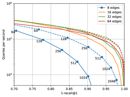
Figure 8 compares the speed vs. accuracy for the NSG and HNSW indexes. The main build-time hyper-parameter of the two methods is the number of edges per node, so we tested several settings (for HNSW this is the number of edges on the base level of the hierachical graph). The main search-time parameter is the number of graph traversal steps during search (parameter efSearch for HNSW and search_L for NSG), which we vary to plot each curve. Increasing the number of edges improves the results only to some extent: beyond 64 edges it degrades. NSG obtains better tradeoffs in general, at the cost of a longer build time. Building the input k-NN graph with NN-descent for 1M vectors takes 37 s, and about the same time with brute force search on a GPU (but in that case the k-NN graph is exact). The NSG graph is frozen after the first batch of vectors is added, there is no easy way to add more vectors afterwards.
IVF vs. graph-based.
An IVF index can be seen as a special case of graph-based index, especially if a small graph-based index is used as coarse quantizer. In Faiss, graph-based indices are a good option for indexes where there is no constraint on memory usage, typically for indexes below 1M vectors. Beyond 10M vectors, the construction time typically becomes the limiting factor. For larger indexes, where compression is required to even fit the database vectors in memory, IVF indexes are the only option. However, as shown in Section 5.1, the optimal number of centroids is so large that a graph-based index should be used to perform the coarse quantization, and much of the search time is spent in the coarse quantization.
6 Database operations
In all the experiments above, the indexes are built in one go with all the vectors, while search operations are performed with one batch containing all query vectors. In real settings, the index evolves over time, vectors may be dynamically added or removed, searches may have to take into account metadata, etc. In this section we show how Faiss supports these operations to some extent, mainly on IVF indexes. When more fine-grained control is required, there are specific APIs to interface with external storage (Section 7.4).
6.1 Identifier-based operations
Faiss indexes support two types of identifiers: sequential ids are based on the order of additions in the index. On the other hand, the user can provide arbitrary 63-bit integer ids along with each vector. The corresponding addition methods for the index are add and add_with_ids. In addition, Faiss supports removing vectors (remove_ids) and updating vector them (update_vectors) by passing the corresponding ids.
Unlike e.g. Usearch [Vardanian, 2022], Faiss does not store arbitrary metadata with the vectors, only 63-bit integer ids can be used (the sign bit is reserved for invalid results).
Flat indexes.
Sequential indexes (IndexFlatCodes) store vectors as a flat array.
They support only sequential ids.
When arbitrary ids are needed, the index can be embedded in a IndexIDMap, that translates sequence numbers to arbitrary ids using a int64 array.
This enables add_with_ids and returns the arbitrary ids at search time.
To also perform id-based operations, a more powerful wrapper class, IndexIDMap2, uses a hash table that maps arbitrary ids back to the sequential ids.
Since graph indexes rely on an embedded IndexFlatCodes to store the actual vectors, they should also be wrapped with the mapping classes. Note however that HNSW does not support suppression and mutation, and that NSG does not even support adding vectors incrementally. Supporting this requires heuristics to re-build the graph when it is mutated, which are implemented in HNSWlib and [Singh et al., 2021] but could be suboptimal indexing-wise.
IVF indexes.
The IVF indexing structure does supports user-provided ids natively at addition and search time. However, id-based access may require a sequential scan, since the entries are stored in an arbitrary order in the inverted lists. Therefore, the IVF index can optionally maintain a DirectMap, that maps user-visible ids to the inverted list and the offset they are stored in. The map can be an array, which is appropriate for sequential ids, or a hash table, for arbitrary 63-bit ids. Obviously, the direct map incurs a memory overhead and an add-time computation overhead, therefore it is disabled by default. When the direct map is enabled, lookup, removal and update are supported.
6.2 Filtered search
Vector filtering consists in returning only database vectors based on some search-time criterion, other vectors are ignored. Faiss has basic support for vector filtering: the user can provide a predicate (IDSelector callback), and if the predicate returns false on the vector id, the vector is ignored.
Therefore, if metadata is needed to filter the vectors, the callback function needs to do an indirection to the metadata table, which is inefficient. Another approach is to exploit the unused bits of the identifier. If documents are indexed with sequential ids, bits are unused.
This is sufficient to store enumerated types (e.g. . country codes, music genres, license types, etc.), dates (as days since some origin), version numbers, etc. However, it is insufficient for more complex metadata. In the example use case below, we use the available bits to implement a more complex filtering method.
Filtering with bag-of-word vectors.
444This example is from the the BigANN’23 challenge, https://big-ann-benchmarks.com/neurips23.html.Each query and database vector has is associated with a few terms from a fixed vocabulary of size (for the queries there are only 1 or 2 words). The filtering consists in considering only the database vectors that include all the query terms. This metadata is given as a sparse matrix .
The basic implementation of the filter uses query vector and the associated words . Before computing a distance to a vector with id , it fetches row of to verify that and are in it. This predicate is relatively slow because (1) it requires to access , which causes cache misses and (2) it performs an iterative binary search. Since the callback is called in the tightest inner loop of the search function, and since the IVF search tends to perform many vector comparisons, this has non negligible performance impact.
To speed up this test, we can use a nifty piece of bit manipulation. In this example, , so we use only bits of the ids, leaving bits that are always 0. We associate to each word a 39-bit signature , and the to each set of words the binary “or” of these signatures. The query is represented by . Database entry with words is represented by . Then we have the following implication: if then all 1 bits of are also set to 1 in :
| (19) |
which is equivalent to:
| (20) |
This binary test is very cheap to perform: a few machine instructions on data that is already in machine registers. It can thus be used as a pre-filter to apply the full membership test on candidates.
The remaining degree of freedom is how to choose the binary signatures, because this rule is always valid, but its filtering ability depends on the choice of the signatures . We experimented with iid Bernouilli bits with varying .
| = probability of 1 | 0.05 | 0.1 | 0.2 | 0.5 |
|---|---|---|---|---|
| Filter hit rate | 75.4% | 82.1% | 76.4% | 42.0% |
i.e. the best setting avoids to do the full check more than 4/5th of the times.
Pre- or post-filtering.
There are two possible approaches to filtered search: post-filtering, which is described above, and pre-filtering, where only vectors with appropriate metadata are considered in vector search. The pre-filtering generates a subset of vectors to compare with.
Therefore, the decision to use pre- or post-filtering depends on whether the subset of vectors is large or not. This can be estimated prior to the search depending on the filtering ability of the query metadata.
In the bag-of-words example, pre-filtering can exploit a term-based inverted file, which is the represented in compressed sparse column format. The product of the frequencies of and is an estimate of what fraction of vectors pre-filtering will perform.
7 Faiss engineering
Faiss started in a research environment. As a consequence, it grew organically, one index at a time, as indexing research was making progress. In the following, we briefly mention the guiding principles that kept the library coherent, how optimization is performed and an example of how Faiss internals are exposed so that it can be embedded in a vector database.
7.1 Code structure
The core of Faiss is implemented in C++. The guiding principles are (1) the code should be as open as possible, so that users can access all the implementation details of the indexes; (2) Faiss should be easy to embed from external libraries; (3) the core library focuses on vector search only.
Therefore, all fields of the classes are public (C++ struct).
Faiss is a late adopter for C++ standards, so that it can be used with relatively old compilers (currently C++17).
Faiss’s basic data types are concrete (not templates): vectors are always represented as 32-bit floats that are portable and provide a good tradeoff between size and accuracy. Similarly, all vector ids are represented with 64-bit integers. This is often larger than necessary for sequential numbering but is widely used for database identifiers.
7.2 High-level interface
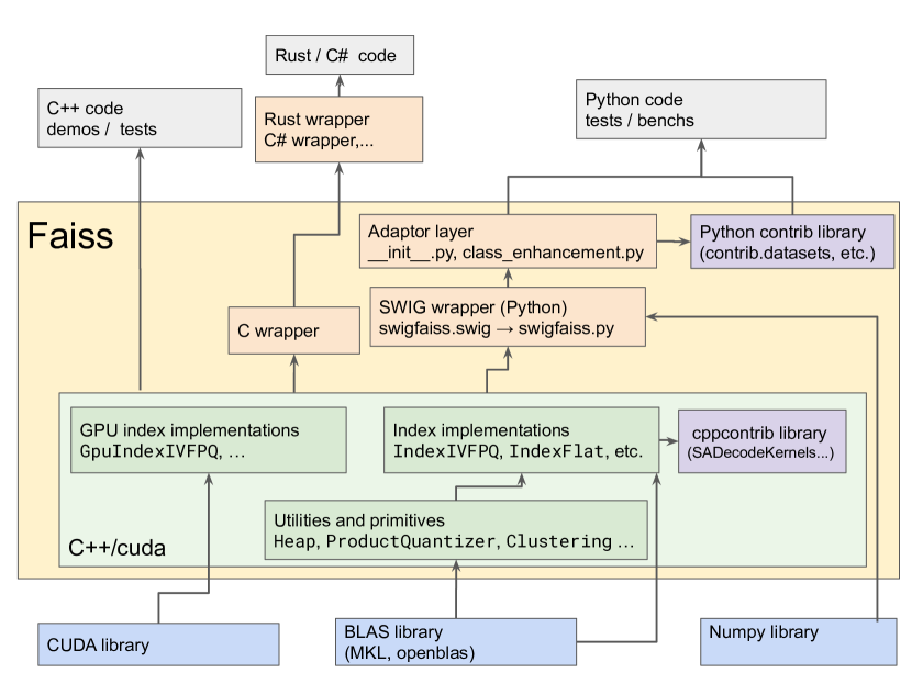
Figure 9 shows the structure of the library. The C++ core library and the GPU add-on have as few dependencies as possible: only a BLAS implementation and CUDA itself.
In order to facilitate experimentation, the whole library is wrapped for scripting languages such as Python with numpy. To this end, SWIG555https://www.swig.org/ exhaustively generates wrappers for all C++ classes, methods and variables. The associated Python layer also contains benchmarking code, dataset definitions, driver code. More and more functionality is embedded in the contrib package of Faiss. Faiss also provides a pure C API, which is useful for producing bindings for programming languages such as Rust or Java.
The Index is presented to the end user as a monolithic object, even when it embeds other indexes as quantizers, refinement indexes or sharded sub-indexes. Therefore, an index can be duplicated with clone_index and serialized into as a single byte stream using a single function, write_index. It also contains the necessary headers so that it can be read by a generic function, read_index.
Index objects can be instantiated explicitly in C++ or Python, but it is more common to build them with the index_factory function.
This function takes a string that describes the index structure and its main parameters.
For example, the string PCA160,IVF20000_HNSW,PQ20x10,RFlat instantiates an IVF index with , where the coarse quantizer is a HNSW index; then the vectors are represented with a PQ20x10 product quantizer. The data is preprocessed with a PCA to 160 dimensions, and the search results are re-ranked with a refinement index that performs exact distance computations.
All the index parameters are set to reasonable defaults, e.g. the PQ encodes the residual of the vectors w.r.t. the coarse quantization centroids.
Faiss provides dedicated standalone vector codec functions sa_encode, sa_decode and sa_code_size as a part of Index API.
7.3 Optimization
Approach to optimization.
Faiss aims at being feature complete first. A non-optimal version of all indexes is implemented first. Code is optimized only when it appears that runtime is important for a certain index. The non-optimized setting is used to control the correctness of the optimized version.
Often, only a subset of data sizes are optimized. For example, for PQ indexes, only and and are fully optimized. For IndexLSH search, only code sizes 4, 8, 16, 20 are optimized. Fixing these sizes allows to write “kernels”, sequences of instructions without explicit loops or tests, that aim to maximize arithmetic throughput.
When generic scalar CPU optimizations are exhausted, Faiss also optimizes specifically for some hardware platforms.
CPU vectorization.
Modern CPUs support Single Instruction, Multiple Data (SIMD) operations, specifically AVX/AVX2 for x86 and NEON for ARM. Faiss exploits those at three levels.
When operations are simple enough (e.g. elementwise vector sum), the code is written in a way that the compiler can vectorize the code by itself, which often boils down to adding restrict keywords to signal that arrays are not overlapping.
The second level leverages SIMD variables and instructions through C++ compiler extensions. Faiss includes simdlib, a collection of classes intended as a layer above the AVX and NEON instruction sets. However, much of the SIMD is done specifically for one instruction set – most often AVX – because it is more efficient.
The third level of optimization is to adapt the data layout and algorithms in order to speed up their SIMD implementation. The 4-bit product and additive quantizer implementations are implemented in this way, inspired by the SCANN library [Guo et al., 2020]: the layout of the PQ codes for several consecutive vectors is interleaved in memory so that a vector permutation can be used to perform the LUT lookups of Equation (14) in parallel. This is implemented in the FastScan variants of PQ and AQ indexes (IndexPQFastScan, IndexIVFResidualQuantizerFastScan, etc.).
GPU Faiss.
Porting Faiss to the GPU is an involved undertaking due to substantial architectural specificities. The implementation of GPU Faiss is detailed in [Johnson et al., 2019], we summarize the GPU implementation challenges therein.
Modern multi-core CPUs are highly latency optimized: they employ an extensive cache hierarchy, branch prediction, speculative execution and out-of-order code execution to improve serial program execution. In contrast, GPUs have a limited cache hierarchy and omit many of these latency optimizations. They instead possess a larger number of concurrent threads of execution (Nvidia’s A100 GPU allows for up to 6,912 warps, each roughly equivalent to a 32-wide vector SIMD CPU thread of execution), a large number of floating-point and integer arithmetic functional units (A100 has up to 19.5 teraflops per second of fp32 fused-multiply add throughput), and a massive register set to allow for a high number of long latency pending instructions in flight (A100 has 27 MiB of register memory). They are thus largely throughput-optimized machines.
The algorithmic techniques used in vector search can be grouped into three broad categories: distance computation of floating-point or binary vectors (which may have been produced via dequantization from a compressed form), table lookups (as seen in PQ distance computations) or scanning (as seen when traversing IVF lists), and irregular, sequential computations such as linked-list traversal (as used in graph-based indices) or ranking the closest vectors.
Distance computation is easy on GPUs and readily exceeds CPU performance, as GPUs are optimized for matrix-matrix multiplication such as that seen in IndexFlat or IVFFlat. Table lookups and list scanning can also be made performant on GPUs, as it is possible to stage small tables (as seen in product quantization) in shared memory (roughly a user-controlled L1 cache) or register memory and perform lookups in parallel across all warps.
Sequential table scanning in IVF indices requires loading data from main (global) memory. While latencies to access main memory are high, for table scanning we know in advance what data we wish to access, so the data movement from main memory into registers can be pipelined or use double buffering, so we can achieve close to peak possible performance.
Selecting the closest vectors to a query vector by ranking distances on the CPU is best implemented with a min- or max-heap. On the GPU, the sequential operations involved in heap operations would similarly force the GPU into a latency-bound regime. This is the largest challenge for GPU implementation of vector search, as the time needed for the heap implementation an order of magnitude greater than all other arithmetic. To handle this, we developed an efficient GPU -selection algorithm [Johnson et al., 2019] that allows for ranking candidate vectors in a single pass, operating at a substantial fraction of peak possible performance per memory bandwidth limits. It relies upon heavy usage of the high-speed, large register memory on GPUs, and small-set bitonic sorting via warp shuffles with buffering techniques.
Irregular computations such as walking graph structures for graph-based indices like HNSW tend to remain in the latency-bound (due to the sequential traversal) rather than arithmetic throughput or memory bandwidth-bound regimes. Here, GPUs are at a disadvantage as compared to CPUs, and emerging techniques such as CAGRA [Ootomo et al., 2023] are required to parallelize otherwise sequential operations with graph traversal.
GPU Faiss implements brute-force GpuIndexFlat as well as the IVF indices GpuIndexIVFFlat, GpuIndexIVFScalarQuantizer and GpuIndexIVFPQ, which are the most useful for large-scale indexing. The coarse quantizer for the IVF indices can be on either CPU or GPU. The GPU index objects have the same interface as their CPU counterparts and the functions index_cpu_to_gpu / index_gpu_to_cpu convert between them. Multiple GPUs are also supported. GPU indexes can take inputs and outputs in GPU or CPU memory as input and output, and Python interface can handle Pytorch tensors.
Advanced options for Faiss components and indices
Many Faiss components expose internal parameters to fine-tune the tradeoff between metrics: number of iterations of k-means, batch sizes for brute-force distance computations, etc. Default parameter values were chosen to work reasonably well in most cases.
Multi-threading
Faiss relies on OpenMP to handle multi-threading. By default, Faiss switches to multi-threading processing if it is beneficial, for example, at training and batch addition time. Faiss multi-threading behavior may be controlled with standard OpenMP environment variables and functions, such as omp_set_num_threads.
When searching a single vector, Faiss does not spawn multiple threads. However, when batched queries are provided, Faiss processes them in parallel, exploiting the effectiveness of the CPU cache and batched linear algebra operations. This is faster than calling search from multiple threads. Therefore, queries should be submitted by batches if possible.
7.4 Interfacing with external storage
Faiss indexes are based on simple storage classes, mainly std::vector to make copy-construction easier.
The default implementation of IndexIVF is based on this storage.
However, to give vector database developers more control over the storage of inverted lists, Faiss provides two lower-level APIs.
Arbitrary inverted lists.
The IVF index uses an abstract InvertedLists object as its storage. The object exposes routines to read one inverted list, add entries to it and remove entries. The default ArrayInvertedLists uses in-memory storage. Alternatively, OnDiskInvertedLists provides memory-mapped storage.
More complex implementations can access a key-value storage either by storing the entire inverted list as a value, or by utilizing key prefix scan operations like the one supported by RocksDB to treat multiple keys prefixed by the same identifier as one inverted list. To this end, the InvertedLists implementation exposes an InvertedListsIterator and fetches the codes and ids from the underlying key-value store, which usually exposes a similar iterable interface. Adding, updating and removing codes can be delegated to the underlying key-value store. We provide an implementation for RocksDB in rocksdb_ivf.
Scanner objects.
With the abstraction above, the scanning loop is still controlled by Faiss. If the calling code needs to control the looping code, then the Faiss IVF index provides an InvertedListScanner object. The scanner’s state includes the current query vector and current inverted list. It provides a distance_to_code method that, given a code, computes the distance from the query to the decompressed vector. At a slightly higher level, it loops over a set of codes and updates a provided result buffer.
This abstraction is useful when the inverted lists are not stored sequentially or fragmented into sub-lists because of metadata filtering [Huang et al., 2020]. Faiss is used only to perform the coarse quantization and the vector encoding.
8 Faiss applications
Faiss is used in many configurations. Hundreds of vector search applications rely on it, both within Meta and externally. Below we present a few use cases that showcase either an extreme scale or an application with particular impact.
8.1 Trillion scale index
For this example, Faiss is used to index 1.5 trillion vectors in 144 dimensions.
The indexing needs to be accurate, therefore the compression of the vectors is limited to 54 bytes with a PCA to 72 dimensions and 6-bit scalar quantizer (PCAR72,SQ6).
A HNSW coarse quantizer with 10M centroids is used for the IndexIVFScalarQuantizer, trained with a simple distributed GPU k-means (implemented in faiss.clustering).
After the training is finished, the index is built in 3 phases:
-
1.
shard over ids: add the input vectors in 2000 shards independently, producing 2000 indexes (that fit in RAM);
-
2.
shard over lists: build the 100 indexes corresponding each to a subset of 100k inverted lists. This is done on 100 different machines, each accessing the 2000 sharded indices, and writing the results directly to a shared disk partition;
-
3.
load the shards: memory-map all 100 indices on a central machine as 100 OnDiskInvertedLists (a memory map of 83TiB).
The central machine that processes queries performs the coarse quantization and loads the inverted lists from the distributed disk partition.
The limiting factor is the network bandwidth of the central machine. Therefore, it is more efficient to distribute the search on 20 intermediate servers to spread the load. This brings the search time down to roughly 1 s per query.
This index is built on vanilla Faiss in pure Python, on commodity CPU servers with hard disk drives and a regular IP network.
8.2 Text retrieval
Faiss is commonly used for natural language processing tasks. In particular, ANNS is relevant for information retrieval [Thakur et al., 2021, Petroni et al., 2021], with applications such as fact checking, entity linking, slot filling or open-domain question answering: these often rely on retrieving relevant content across a large-scale corpus. To that end, embedding models have been optimized for text retrieval [Izacard et al., 2021, Lin et al., 2023a].
Finally, [Izacard et al., 2023], [Lin et al., 2023b], [Shi et al., 2023b] and [Khandelwal et al., 2020] consist of language models that have been trained to integrate textual retrieval in order to improve their accuracy, factuality or compute efficiency.
8.3 Data mining
Another recurrent application of ANNS and Faiss is in the mining and curation of large datasets. In particular, Faiss has been used to mine bilingual texts across very large text datasets retrieved from the web [Schwenk and Douze, 2017, Barrault et al., 2023], or to organize a language model’s training corpus in order to group together series of documents covering similar topics [Shi et al., 2023a].
In the image domain, [Oquab et al., 2023] leverages Faiss to remove duplicates from a dataset containing 1.3B images. It then relies on efficient indexing in order to mine a curated dataset whose distribution matches the distribution of a target dataset.
8.4 Content Moderation
One of the major applications of Faiss is the detection and remediation of harmful content at scale. Human labelled examples of policy violating images and videos are embedded with models such as SSCD [Pizzi et al., 2022] and stored in a Faiss index. To decide if a new image or video would violate some policies, a multi-stage classification pipeline first embeds the content and searches the Faiss index for similar labelled examples, typically utilizing range queries. The results are aggregated and processed through additional machine classification or human verification. Since the impact of mistakes is high, good representations should discriminate perceptually similar and different content, and accurate similarity search is required even at billions to trillion-scale. The former problem motivated the Image and Video Similarity Challenges [Douze et al., 2021, Pizzi et al., 2023].
9 Conclusion
In this work, we presented the task of efficient approximate nearest-neighbor vector search, and exposed how Faiss addresses the most common practitioners’ problems in that space. Indeed, Faiss contains a wide set of methods that, once combined, achieve varying tradeoffs in terms of training time, throughput, memory usage and accuracy. Most of the use cases and experiments mentioned in this paper are presented in more detail and with corresponding code in Faiss’ wiki pages.
References
- [Amara et al., 2022] Amara, K., Douze, M., Sablayrolles, A., and Jégou, H. (2022). Nearest neighbor search with compact codes: A decoder perspective. In ICMR.
- [Aumüller et al., 2020] Aumüller, M., Bernhardsson, E., and Faithfull, A. (2020). Ann-benchmarks: A benchmarking tool for approximate nearest neighbor algorithms. Information Systems, 87:101374.
- [Babenko and Lempitsky, 2014] Babenko, A. and Lempitsky, V. (2014). Additive quantization for extreme vector compression. In Conference on Computer Vision and Pattern Recognition.
- [Babenko and Lempitsky, 2015] Babenko, A. and Lempitsky, V. (2015). Tree quantization for large-scale similarity search and classification. In Proceedings of the IEEE Conference on Computer Vision and Pattern Recognition, pages 4240–4248.
- [Babenko and Lempitsky, 2016] Babenko, A. and Lempitsky, V. (2016). Efficient indexing of billion-scale datasets of deep descriptors. In Conference on Computer Vision and Pattern Recognition.
- [Bachrach et al., 2014] Bachrach, Y., Finkelstein, Y., Gilad-Bachrach, R., Katzir, L., Koenigstein, N., Nice, N., and Paquet, U. (2014). Speeding up the xbox recommender system using a euclidean transformation for inner-product spaces. In Proceedings of the 8th ACM Conference on Recommender systems, pages 257–264.
- [Baranchuk et al., 2023] Baranchuk, D., Douze, M., Upadhyay, Y., and Yalniz, I. Z. (2023). Dedrift: Robust similarity search under content drift. In Proceedings of the IEEE/CVF International Conference on Computer Vision, pages 11026–11035.
- [Barrault et al., 2023] Barrault, L., Chung, Y.-A., Meglioli, M. C., Dale, D., Dong, N., Duquenne, P.-A., Elsahar, H., Gong, H., Heffernan, K., Hoffman, J., et al. (2023). Seamlessm4t-massively multilingual & multimodal machine translation. arXiv preprint arXiv:2308.11596.
- [Bojanowski et al., 2017] Bojanowski, P., Grave, E., Joulin, A., and Mikolov, T. (2017). Enriching word vectors with subword information. Transactions of the association for computational linguistics, 5:135–146.
- [Boytsov et al., 2016] Boytsov, L., Novak, D., Malkov, Y., and Nyberg, E. (2016). Off the beaten path: Let’s replace term-based retrieval with k-nn search. In Proceedings of the 25th ACM international on conference on information and knowledge management, pages 1099–1108.
- [Bruch et al., 2023] Bruch, S., Nardini, F. M., Ingber, A., and Liberty, E. (2023). An approximate algorithm for maximum inner product search over streaming sparse vectors. arXiv preprint arXiv:2301.10622.
- [Cao et al., 2017] Cao, Z., Long, M., Wang, J., and Yu, P. S. (2017). Hashnet: Deep learning to hash by continuation. In Proceedings of the IEEE International Conference on Computer Vision (ICCV).
- [Caron et al., 2018] Caron, M., Bojanowski, P., Joulin, A., and Douze, M. (2018). Deep clustering for unsupervised learning of visual features. In Proceedings of the European conference on computer vision (ECCV), pages 132–149.
- [Caron et al., 2021] Caron, M., Touvron, H., Misra, I., Jégou, H., Mairal, J., Bojanowski, P., and Joulin, A. (2021). Emerging properties in self-supervised vision transformers. In Proceedings of the IEEE/CVF international conference on computer vision, pages 9650–9660.
- [Charikar, 2002] Charikar, M. (2002). Similarity estimation techniques from rounding algorithms. In Proc. ACM symp. Theory of computing.
- [Chen et al., 2020] Chen, T., Kornblith, S., Norouzi, M., and Hinton, G. (2020). A simple framework for contrastive learning of visual representations. In Proceedings of the 37th International Conference on Machine Learning, Proceedings of Machine Learning Research, pages 1597–1607. PMLR.
- [Chen et al., 2010] Chen, Y., Guan, T., and Wang, C. (2010). Approximate nearest neighbor search by residual vector quantization. Sensors, 10(12):11259–11273.
- [Chern et al., 2022] Chern, F., Hechtman, B., Davis, A., Guo, R., Majnemer, D., and Kumar, S. (2022). Tpu-knn: K nearest neighbor search at peak flop/s. Advances in Neural Information Processing Systems, 35:15489–15501.
- [Datar et al., 2004] Datar, M., Immorlica, N., Indyk, P., and Mirrokni, V. S. (2004). Locality-sensitive hashing scheme based on p-stable distributions. In Proceedings of the twentieth annual symposium on Computational geometry, pages 253–262.
- [Devlin et al., 2018] Devlin, J., Chang, M.-W., Lee, K., and Toutanova, K. (2018). Bert: Pre-training of deep bidirectional transformers for language understanding. arXiv preprint arXiv:1810.04805.
- [Dhillon and Modha, 2001] Dhillon, I. S. and Modha, D. S. (2001). Concept decompositions for large sparse text data using clustering. Machine learning, 42:143–175.
- [Dong et al., 2011] Dong, W., Moses, C., and Li, K. (2011). Efficient k-nearest neighbor graph construction for generic similarity measures. In Proceedings of the 20th international conference on World wide web, pages 577–586.
- [Douze and Jégou, 2014] Douze, M. and Jégou, H. (2014). The yael library. In Proceedings of the 22nd ACM international conference on Multimedia, pages 687–690.
- [Douze et al., 2016] Douze, M., Jégou, H., and Perronnin, F. (2016). Polysemous codes. In European Conference on Computer Vision.
- [Douze et al., 2018] Douze, M., Sablayrolles, A., and Jégou, H. (2018). Link and code: Fast indexing with graphs and compact regression codes. In Proceedings of the IEEE conference on computer vision and pattern recognition, pages 3646–3654.
- [Douze et al., 2021] Douze, M., Tolias, G., Pizzi, E., Papakipos, Z., Chanussot, L., Radenovic, F., Jenicek, T., Maximov, M., Leal-Taixé, L., Elezi, I., et al. (2021). The 2021 image similarity dataset and challenge. arXiv preprint arXiv:2106.09672.
- [Duquenne et al., 2023] Duquenne, P.-A., Schwenk, H., and Sagot, B. (2023). Sentence-level multimodal and language-agnostic representations. arXiv preprint arXiv:2308.11466.
- [Fu et al., 2017] Fu, C., Xiang, C., Wang, C., and Cai, D. (2017). Fast approximate nearest neighbor search with the navigating spreading-out graph. arXiv preprint arXiv:1707.00143.
- [Ge et al., 2013] Ge, T., He, K., Ke, Q., and Sun, J. (2013). Optimized product quantization for approximate nearest neighbor search. In Conference on Computer Vision and Pattern Recognition.
- [Gollapudi et al., 2023] Gollapudi, S., Karia, N., Sivashankar, V., Krishnaswamy, R., Begwani, N., Raz, S., Lin, Y., Zhang, Y., Mahapatro, N., Srinivasan, P., Singh, A., and Simhadri, H. V. (2023). Filtered-diskann: Graph algorithms for approximate nearest neighbor search with filters. In Proceedings of the ACM Web Conference 2023.
- [Gong et al., 2012] Gong, Y., Lazebnik, S., Gordo, A., and Perronnin, F. (2012). Iterative quantization: A procrustean approach to learning binary codes for large-scale image retrieval. IEEE Trans. Pattern Analysis and Machine Intelligence.
- [Guo et al., 2020] Guo, R., Sun, P., Lindgren, E., Geng, Q., Simcha, D., Chern, F., and Kumar, S. (2020). Accelerating large-scale inference with anisotropic vector quantization. In International Conference on Machine Learning. PMLR.
- [Hong et al., 2019] Hong, W., Tang, X., Meng, J., and Yuan, J. (2019). Asymmetric mapping quantization for nearest neighbor search. IEEE Transactions on Pattern Analysis and Machine Intelligence, 42(7):1783–1790.
- [Huang et al., 2020] Huang, J.-T., Sharma, A., Sun, S., Xia, L., Zhang, D., Pronin, P., Padmanabhan, J., Ottaviano, G., and Yang, L. (2020). Embedding-based retrieval in facebook search. In Proceedings of the 26th ACM SIGKDD International Conference on Knowledge Discovery & Data Mining, pages 2553–2561.
- [Izacard et al., 2021] Izacard, G., Caron, M., Hosseini, L., Riedel, S., Bojanowski, P., Joulin, A., and Grave, E. (2021). Unsupervised dense information retrieval with contrastive learning.
- [Izacard et al., 2023] Izacard, G., Lewis, P., Lomeli, M., Hosseini, L., Petroni, F., Schick, T., Dwivedi-Yu, J., Joulin, A., Riedel, S., and Grave, E. (2023). Atlas: Few-shot learning with retrieval augmented language models. Journal of Machine Learning Research, 24(251):1–43.
- [Jaiswal et al., 2022] Jaiswal, S., Krishnaswamy, R., Garg, A., Simhadri, H. V., and Agrawal, S. (2022). Ood-diskann: Efficient and scalable graph anns for out-of-distribution queries.
- [Jegou et al., 2008] Jegou, H., Douze, M., and Schmid, C. (2008). Hamming embedding and weak geometric consistency for large scale image search. In Computer Vision–ECCV 2008: 10th European Conference on Computer Vision, Marseille, France, October 12-18, 2008, Proceedings, Part I 10, pages 304–317. Springer.
- [Jégou et al., 2010] Jégou, H., Douze, M., and Schmid, C. (2010). Product quantization for nearest neighbor search. IEEE Trans. Pattern Analysis and Machine Intelligence.
- [Jégou et al., 2011a] Jégou, H., Perronnin, F., Douze, M., Sánchez, J., Pérez, P., and Schmid, C. (2011a). Aggregating local image descriptors into compact codes. IEEE transactions on pattern analysis and machine intelligence, 34(9):1704–1716.
- [Jégou et al., 2011b] Jégou, H., Tavenard, R., Douze, M., and Amsaleg, L. (2011b). Searching in one billion vectors: re-rank with source coding. In International Conference on Acoustics, Speech, and Signal Processing.
- [Johnson et al., 2019] Johnson, J., Douze, M., and Jégou, H. (2019). Billion-scale similarity search with GPUs. IEEE Trans. on Big Data.
- [Khandelwal et al., 2020] Khandelwal, U., Levy, O., Jurafsky, D., Zettlemoyer, L., and Lewis, M. (2020). Generalization through memorization: Nearest neighbor language models.
- [Lin et al., 2023a] Lin, S.-C., Asai, A., Li, M., Oguz, B., Lin, J., Mehdad, Y., tau Yih, W., and Chen, X. (2023a). How to train your dragon: Diverse augmentation towards generalizable dense retrieval.
- [Lin et al., 2023b] Lin, X. V., Chen, X., Chen, M., Shi, W., Lomeli, M., James, R., Rodriguez, P., Kahn, J., Szilvasy, G., Lewis, M., Zettlemoyer, L., and Yih, S. (2023b). Ra-dit: Retrieval-augmented dual instruction tuning. ArXiv, abs/2310.01352.
- [Liu et al., 2015] Liu, S., Lu, H., and Shao, J. (2015). Improved residual vector quantization for high-dimensional approximate nearest neighbor search. arXiv preprint arXiv:1509.05195.
- [Lloyd, 1982] Lloyd, S. (1982). Least squares quantization in PCM. IEEE Transactions on Information Theory.
- [Lowe, 2004] Lowe, D. G. (2004). Distinctive image features from scale-invariant keypoints. International Journal of Computer Vision, 60(2).
- [Lv et al., 2004] Lv, Q., Charikar, M., and Li, K. (2004). Image similarity search with compact data structures. In Proceedings of the thirteenth ACM international conference on Information and knowledge management, pages 208–217.
- [Malkov and Yashunin, 2018] Malkov, Y. A. and Yashunin, D. A. (2018). Efficient and robust approximate nearest neighbor search using hierarchical navigable small world graphs. IEEE transactions on pattern analysis and machine intelligence, 42(4):824–836.
- [Martinez et al., 2016] Martinez, J., Clement, J., Hoos, H. H., and Little, J. J. (2016). Revisiting additive quantization. In European Conference on Computer Vision.
- [Martinez et al., 2018] Martinez, J., Zakhmi, S., Hoos, H. H., and Little, J. J. (2018). LSQ++: lower running time and higher recall in multi-codebook quantization. In European Conference on Computer Vision.
- [Matsui et al., 2018] Matsui, Y., Uchida, Y., Jégou, H., and Satoh, S. (2018). A survey of product quantization. ITE Transactions on Media Technology and Applications.
- [Mikolov et al., 2013] Mikolov, T., Chen, K., Corrado, G., and Dean, J. (2013). Efficient estimation of word representations in vector space. arXiv preprint arXiv:1301.3781.
- [Morozov and Babenko, 2018] Morozov, S. and Babenko, A. (2018). Non-metric similarity graphs for maximum inner product search. Advances in Neural Information Processing Systems, 31.
- [Morozov and Babenko, 2019] Morozov, S. and Babenko, A. (2019). Unsupervised neural quantization for compressed-domain similarity search. In International Conference on Computer Vision.
- [Muja and Lowe, 2014] Muja, M. and Lowe, D. G. (2014). Scalable nearest neighbor algorithms for high dimensional data. IEEE transactions on pattern analysis and machine intelligence, 36(11):2227–2240.
- [Ootomo et al., 2023] Ootomo, H., Naruse, A., Nolet, C., Wang, R., Feher, T., and Wang, Y. (2023). Cagra: Highly parallel graph construction and approximate nearest neighbor search for gpus.
- [Oquab et al., 2023] Oquab, M., Darcet, T., Moutakanni, T., Vo, H. V., Szafraniec, M., Khalidov, V., Fernandez, P., Haziza, D., Massa, F., El-Nouby, A., Howes, R., Huang, P.-Y., Xu, H., Sharma, V., Li, S.-W., Galuba, W., Rabbat, M., Assran, M., Ballas, N., Synnaeve, G., Misra, I., Jegou, H., Mairal, J., Labatut, P., Joulin, A., and Bojanowski, P. (2023). DINOv2: Learning robust visual features without supervision.
- [Paterek, 2007] Paterek, A. (2007). Improving regularized singular value decomposition for collaborative filtering. In Proceedings of KDD cup and workshop.
- [Paulevé et al., 2010] Paulevé, L., Jégou, H., and Amsaleg, L. (2010). Locality sensitive hashing: A comparison of hash function types and querying mechanisms. Pattern recognition letters, 31(11):1348–1358.
- [Petroni et al., 2021] Petroni, F., Piktus, A., Fan, A., Lewis, P., Yazdani, M., De Cao, N., Thorne, J., Jernite, Y., Karpukhin, V., Maillard, J., Plachouras, V., Rocktäschel, T., and Riedel, S. (2021). KILT: a benchmark for knowledge intensive language tasks. In Proceedings of the 2021 Conference of the North American Chapter of the Association for Computational Linguistics: Human Language Technologies, Online. Association for Computational Linguistics.
- [Pizzi et al., 2023] Pizzi, E., Kordopatis-Zilos, G., Patel, H., Postelnicu, G., Ravindra, S. N., Gupta, A., Papadopoulos, S., Tolias, G., and Douze, M. (2023). The 2023 video similarity dataset and challenge. arXiv preprint arXiv:2306.09489.
- [Pizzi et al., 2022] Pizzi, E., Roy, S. D., Ravindra, S. N., Goyal, P., and Douze, M. (2022). A self-supervised descriptor for image copy detection. In Proceedings of the IEEE/CVF Conference on Computer Vision and Pattern Recognition, pages 14532–14542.
- [Radford et al., 2021] Radford, A., Kim, J. W., Hallacy, C., Ramesh, A., Goh, G., Agarwal, S., Sastry, G., Askell, A., Mishkin, P., Clark, J., et al. (2021). Learning transferable visual models from natural language supervision. In International conference on machine learning, pages 8748–8763. PMLR.
- [Sandhawalia and Jégou, 2010] Sandhawalia, H. and Jégou, H. (2010). Searching with expectations. In International Conference on Acoustics, Speech, and Signal Processing.
- [Schwenk and Douze, 2017] Schwenk, H. and Douze, M. (2017). Learning joint multilingual sentence representations with neural machine translation. In Proceedings of the 2nd Workshop on Representation Learning for NLP, pages 157–167, Vancouver, Canada. Association for Computational Linguistics.
- [Shi et al., 2023a] Shi, W., Min, S., Lomeli, M., Zhou, C., Li, M., Lin, V., Smith, N. A., Zettlemoyer, L., Yih, S., and Lewis, M. (2023a). In-context pretraining: Language modeling beyond document boundaries. ArXiv, abs/2310.10638.
- [Shi et al., 2023b] Shi, W., Min, S., Yasunaga, M., Seo, M., James, R., Lewis, M., Zettlemoyer, L., and tau Yih, W. (2023b). Replug: Retrieval-augmented black-box language models.
- [Simhadri et al., 2022a] Simhadri, H. V., Williams, G., Aumüller, M., Douze, M., Babenko, A., Baranchuk, D., Chen, Q., Hosseini, L., Krishnaswamny, R., Srinivasa, G., et al. (2022a). Results of the neurips’21 challenge on billion-scale approximate nearest neighbor search. In NeurIPS 2021 Competitions and Demonstrations Track, pages 177–189. PMLR.
- [Simhadri et al., 2022b] Simhadri, H. V., Williams, G., Aumüller, M., Douze, M., Babenko, A., Baranchuk, D., Chen, Q., Hosseini, L., Krishnaswamny, R., Srinivasa, G., Subramanya, S. J., and Wang, J. (2022b). Results of the neurips’21 challenge on billion-scale approximate nearest neighbor search. In Proceedings of the NeurIPS 2021 Competitions and Demonstrations Track, volume 176 of Proceedings of Machine Learning Research, pages 177–189. PMLR.
- [Singh et al., 2021] Singh, A., Subramanya, S. J., Krishnaswamy, R., and Simhadri, H. V. (2021). Freshdiskann: A fast and accurate graph-based ann index for streaming similarity search.
- [Subramanya et al., 2019] Subramanya, S. J., Kadekodi, R., Krishaswamy, R., and Simhadri, H. V. (2019). Diskann: Fast accurate billion-point nearest neighbor search on a single node. In Neurips.
- [Sun et al., 2023a] Sun, P., Guo, R., and Kumar, S. (2023a). Automating nearest neighbor search configuration with constrained optimization. arXiv preprint arXiv:2301.01702.
- [Sun et al., 2023b] Sun, P., Simcha, D., Dopson, D., Guo, R., and Kumar, S. (2023b). Soar: Improved quantization for approximate nearest neighbor search. In Thirty-seventh Conference on Neural Information Processing Systems.
- [Szegedy et al., 2015] Szegedy, C., Liu, W., Jia, Y., Sermanet, P., Reed, S., Anguelov, D., Erhan, D., Vanhoucke, V., and Rabinovich, A. (2015). Going deeper with convolutions. In Proceedings of the IEEE conference on computer vision and pattern recognition, pages 1–9.
- [Tavenard et al., 2011] Tavenard, R., Jégou, H., and Amsaleg, L. (2011). Balancing clusters to reduce response time variability in large scale image search. In 2011 9th International Workshop on Content-Based Multimedia Indexing (CBMI), pages 19–24. IEEE.
- [Thakur et al., 2021] Thakur, N., Reimers, N., Rücklé, A., Srivastava, A., and Gurevych, I. (2021). BEIR: A heterogeneous benchmark for zero-shot evaluation of information retrieval models. In Thirty-fifth Conference on Neural Information Processing Systems Datasets and Benchmarks Track (Round 2).
- [van Luijt and Verhagen, 2020] van Luijt, B. and Verhagen, M. (2020). Bringing semantic knowledge graph technology to your data. IEEE Software, 37(2):89–94.
- [Vardanian, 2022] Vardanian, A. (2022). USearch by Unum Cloud.
- [Wang et al., 2015] Wang, J., Liu, W., Kumar, S., and Chang, S.-F. (2015). Learning to hash for indexing big data - a survey. Proc. of the IEEE.
- [Wang et al., 2021] Wang, J., Yi, X., Guo, R., Jin, H., Xu, P., Li, S., Wang, X., Guo, X., Li, C., Xu, X., et al. (2021). Milvus: A purpose-built vector data management system. In Proceedings of the 2021 International Conference on Management of Data, pages 2614–2627.
- [Wang et al., 2017] Wang, J., Zhang, T., Sebe, N., Shen, H. T., et al. (2017). A survey on learning to hash. IEEE transactions on pattern analysis and machine intelligence, 40(4):769–790.
- [Weber et al., 1998] Weber, R., Schek, H.-J., and Blott, S. (1998). A quantitative analysis and performance study for similarity-search methods in high-dimensional spaces. In VLDB, volume 98, pages 194–205.